Resonance phenomena in ultracold dipole-dipole scattering

Abstract

Elastic scattering resonances occurring in ultracold collisions of either bosonic or fermionic polar molecules are investigated. The Born-Oppenheimer adiabatic representation of the two-body dynamics provides both a qualitative classification scheme and a quantitative WKB quantization condition that predicts several sequences of resonant states. It is found that the near-threshold energy dependence of ultracold collision cross sections varies significantly with the particle exchange symmetry, with bosonic systems showing much smoother energy variations than their fermionic counterparts. Resonant variations of the angular distributions in ultracold collisions are also described.

Keywords: dipoles, low-energy scattering, resonances

I Introduction

While numerous advances have been made in the study of dilute atomic gases at ultracold temperatures, very little is yet known about ultracold molecular gases, particularly for strongly polar molecules. The first experiments with ensembles of trapped polar molecules are only recently reported JunYe . Molecular gases are more difficult to cool than their atomic counterparts, and the temperatures at which effects of quantum degeneracy are apparent are typically much lower. Improved cooling and trapping techniques for cold molecules have emerged, including the development of decelerators decelerators and the formation of molecules from ultracold atoms via photoassociation photoassociation . But most trapped molecular ensembles are still relatively “hot” and rather far from the quantum degenerate regime.

Many theoretical studies of molecular collisions at cold and ultracold temperatures are now emerging in order to spur and assist these ongoing experimental efforts Review1 ; theory ; theory1 ; theory2 ; theory3 . One of the most striking outcomes of recent studies is the identification of large elastic scattering resonances in zero-energy collisions of virtually all molecules aligned in an external electric field TickBohn1 . These resonances can be “tuned” with the electric field strength, resulting in a novel kind of zero-energy spectroscopy TickBohn2 , and they have also been predicted in calculations of trapped ensembles Doerte . In an earlier work, we demonstrated the universality of these resonances for bosonic collision partners ourPRL . In this paper, we provide a number of details of the resonance classification, and extend the work by comparing and contrasting with similar resonances in collisions between fermionic polar molecules.

A few general observations highlight the importance that resonance formation and decay will play in the dynamics of ultracold molecular gases: 1) near-threshold collisions of polar molecules are “resonance rich”, with resonances of shape, Feshbach/Fano and mixed characteristics forming in the long-range dipole-dipole field, and with detailed characteristics sensitive to shorter ranged interactions; 2) the resonances occur systematically and can readily be predicted by simple semi-classical quantization formulas; 3) the character and frequency of resonances differ distinctly between bose and fermi collision partners; 4) the angular distribution of scattered products in near-zero energy collisions is strongly correlated with resonance formation and decay; and 5) the resonances are universal and, with minor field variations, can be realized in virtually all strongly polar molecules. This ubiquity of threshold resonance phenomena implies that complex few and many-body processes in ultracold polar gases are likely to emerge as experiments progress to the quantum-degenerate regime.

II Long-range interaction of polar molecules

There are many molecules (such as alkali-halide salts) which, in their lowest energy states, exhibit strong polar characteristics. However, in the absence of external fields, as a consequence of parity conservation, even these strongly ”polar” molecules have zero dipole moment. Molecular interactions may polarize such collision partners, even in the absence of any external fields, though this generally produces a relatively benign and isotropic ($1/r^{6}$) van der Waals attraction at large intermolecular separations. The stronger ($1/r^{3}$) anisotropic interactions of interest here require the imposition of an external electric field, $\vec{\cal E}$, coupling opposite parity states, and producing a generally field-dependent dipole moment

$$\vec{\mu}({\cal E})=-(\frac{dE}{d{\cal E}})\hat{\cal E}$$ (1)

for all molecules.

The magnitude and sign of the ”induced” dipole moment, $\mu$, therefore depends on specific details of the $E({\cal E})$ Stark shift of the state of interest for any particular molecule BohnStark . In general, for zero field, two molecular states of opposite parity are separated by an energy gap, so that $E({\cal E})$ varies quadratically for small fields. At larger fields, Stark maps tend to a linear regime, yielding a maximal induced dipole moment $\vec{\mu}\rightarrow\vec{d}=qs\hat{d}$, where $q$ is some effective charge, and $s$ is a measure of the charge separation along the field axis, and typically is a few Bohr in size. The magnitude of the electric field required to maximize the dipole moment $\mu$ depends principally on the size of the zero-field energy gap; molecules with ground $\Sigma$ states tend to have relatively large gaps and often require experimentally unrealistic field strengths, while those in $\Pi$ or $\Delta$ states can have quite small gaps (owing to the phenomenon of $\Lambda$-doubling), producing maximal dipole moments with modest fields.

For ground vibrational states of $\Sigma$ molecules $\mu({\cal E})$ can be estimated as

$$\vec{\mu}=-({dE\over d{\cal E}})\hat{z}=-d^{2}\frac{\cal E}{3B}\hat{z}\ \ \ ,$$ (2)

where $B$ is the rotational constant of the molecule and $\hat{z}$ is the field direction. In Table LABEL:Tab:SigmaMol we provide typical values of the intrinsic dipole moment $d$ and the rotational constant $B$ for a variety of $\Sigma$-state molecules NIST .

Table 1: Important dipolar and rotational constants of $\Sigma$ molecules. $2.928(-05)$ stands for $2.928\times 10^{-05}$. The dipole length, $D$ is calculated in the assumption that the molecule is completely polarized.

Molecule	$B_{0}$,a.u.	$d$, a.u.	$M/m_{e}$	$D$
HI	2.928(-05)	0.1762	116584.923	3618
H35Cl	4.757(-05)	0.4362	32790.736	6239
H37Cl	4.750(-05)	0.4359	34610.935	6578
H79Br	3.805(-05)	0.3254	72848.241	7715
H81Br	3.803(-05)	0.3254	74669.264	7908
HF	9.368(-05)	0.7187	18234.562	9418
6LiH	3.444(-05)	2.3149	6401.025	34303
6LiD	1.978(-05)	2.3094	7318.190	39029
7LiH	3.374(-05)	2.3143	7313.273	39170
7LiD	1.908(-05)	2.3087	8230.438	43868
SiO	3.300(-06)	1.2190	40077.881	59555
73GeO	2.211(-06)	1.2915	81044.140	135174
74GeO	2.206(-06)	1.2915	81953.505	136690
6LiF	6.820(-06)	2.4895	22798.434	141300
7LiF	6.083(-06)	2.4885	23710.682	146835
Ca35Cl	6.931(-07)	1.6781	68295.833	192320
Ca37Cl	6.731(-07)	1.6781	70116.033	197446
Li35Cl	3.643(-06)	2.7935	37354.608	291510
Li37Cl	3.614(-06)	2.7935	39174.808	305714
NaF	1.980(-06)	3.2089	38269.879	394078
7Li79Br	2.518(-06)	2.4394	78324.361	466093
7Li81Br	2.513(-06)	2.4394	80145.384	476930
KF	1.270(-06)	3.3808	52829.231	603832
Na35Cl	9.899(-07)	3.5416	52826.053	662585
207PbO	1.396(-06)	1.8256	203225.448	677339
208PbO	1.396(-06)	1.8256	204137.580	680380
Na37Cl	9.900(-07)	3.5415	54646.253	685369
6LiI	2.338(-06)	2.9228	121148.795	1034936
7LiI	2.010(-06)	2.9228	122061.043	1042730
K35Cl	5.844(-07)	4.0404	67385.406	1100055
K37Cl	5.677(-07)	4.0403	69205.605	1129704
SrO	1.535(-06)	3.5018	94699.539	1161235
Na79Br	6.870(-07)	3.5876	92883.558	1195526
Na81Br	6.832(-07)	3.5876	94704.581	1218965
BaO	1.421(-06)	3.1295	140271.411	1373829
NaI	5.353(-07)	3.6338	136620.240	1804044
K79Br	3.691(-07)	4.1816	107442.911	1878697
K81Br	3.661(-07)	4.1815	109263.934	1910503
KI	2.768(-07)	4.2572	151179.593	2739934

The wide variety of polar molecules available for trapping (once adequate experimental techniques are developed) is one of several reasons for the intensity of recent interest in the field.

At intermolecular separations much greater than the charge displacement, $r\gg s$, molecular interactions reduce to the familiar dipole-dipole form

$$V(\vec{r})=\frac{d^{2}}{r^{3}}\left[\hat{d}_{1}\cdot\hat{d}_{2}-3(\hat{r}\cdot\hat{d}_{1})(\hat{r}\cdot\hat{d}_{2})\right]$$ (3)

which, for a pair of identical molecules in the same field-aligned state, yields an equation of relative motion

$$\left[-\frac{\hbar^{2}}{2M}\nabla^{2}+\frac{\mu^{2}}{r^{3}}\left(1-3(\hat{r}\cdot\hat{z})^{2}\right)\right]\psi(\vec{r})=E_{{\rm rel}}\psi(\vec{r})$$ (4)

where $\hat{z}$ is the field axis and $M$ is the reduced mass. As noted above, $\mu$ assumes its maximal value of $d$ at large fields, but reduces to zero as ${\cal E}\rightarrow 0$.

Equation (4) is easily written in dimensionless form, independent of $\mu$ and $M$,

$$\left[-\frac{1}{2}\nabla^{2}+\frac{1}{r^{3}}\left(1-3(\hat{r}\cdot\hat{z})^{2}\right)\right]\psi(\vec{r})=E_{{\rm rel}}\psi(\vec{r})\ \ \ .$$ (5)

providing that all distances and energies are measured in dipole units (d.u.)

$$\begin{array}[]{c}D=\mu^{2}M/\hbar^{2}\\ E_{D}=\hbar^{6}/(M^{3}\mu^{4})\end{array}\ \ .$$ (6)

The emergence of these natural length and energy scales, previously noted by many authors Scale , is striking when one recognizes that for maximal $\mu$, $D\sim 10^{2}-10^{6}$ times larger than typical molecular length scales, while $E_{D}\sim 10^{-6}-10^{-12}$ times smaller than typical rotational level splittings. Dipole-dipole interactions dominate the long range part of the interaction in any polar system, suggesting that observable characteristics of polar gases at sufficiently cold temperatures will be universal. Two types of long-range dipole-dipole effects can accordingly be identified: those that do not depend on the short-range boundary conditions and those that result from an interplay between short-range and long-range physics. In this work we model the short-range interaction with a spherically-symmetric ”hard wall” boundary condition at $r=r_{0}\equiv R_{0}/D$.

III Adiabatic representation

Expanding the solutions of Schrödinger’s Eq. (5) in terms of spherical harmonics seems a natural numerical approach with obvious advantages: the symmetries of the dipole-dipole interactions are clearly revealed in the spherical harmonic basis. The interaction conserves the parity of the state and the cylindrical symmetry allows for conservation of the quantum number $m$. The states of a given orbital quantum number $l$ are coupled only to the two states of $l\pm 2$, which leads to a useful tri-diagonal structure of the potential matrix.

In a spherical harmonic representation, however, channel coupling is not small compared to the diagonal elements for the whole range of $l=0\ldots\infty$, and in the case of the s-wave, which is expected to contribute considerably at low energies, the coupling to the d-wave dominates the interaction. It is advantageous, therefore, to change the representation so that an efficient channel decoupling is achieved. For that purpose, we utilize the Born-Oppenheimer adiabatic representation, and diagonalize the angular part of the interaction together with the kinetic centrifugal terms.

For a given value of the interparticle distance $r$ we calculate the eigenstates of the following angular operator $H_{a}$

$$[H_{a}(r)]_{ll^{\prime}}=l(l+1)\delta_{ll^{\prime}}+\frac{1}{r}\langle lm|1-3(\hat{r}\cdot\hat{z})^{2}|l^{\prime}m\rangle\ \ .$$ (7)

As the potential matrix elements

$$\begin{array}[]{rcl}V_{ll^{\prime}}^{(m)}&\equiv&\langle lm|1-3(\hat{r}\cdot\hat{z})^{2}|l^{\prime}m\rangle=\\ &=&(1-\frac{3}{2l+1}(\frac{(l-m)(l+m)}{2l-1}+\frac{(l-m+1)(l+m+1)}{2l+3}))\delta_{l,l^{\prime}}-\\ &&-\frac{3}{2l+3}\sqrt{\frac{((l+1)^{2}-m^{2})((l+2)^{2}-m^{2})}{(2l+1)(2l+5)}}\delta_{l,l^{\prime}-2}\\ &&-\frac{3}{2l-1}\sqrt{\frac{((l-1)^{2}-m^{2})(l^{2}-m^{2})}{(2l-3)(2l+1)}}\delta_{l,l^{\prime}+2}\end{array}$$ (8)

depend on $m^{2}$, all the adiabatic states are doubly degenerate except $m=0$, which is non-degenerate.

Explicitly, we solve the following eigenvalue problem for each $r$

$$H_{a}(r)\phi_{n}(\hat{r};r)=v_{n}(r)\phi_{n}(\hat{r};r)\ \ .$$ (9)

As the off-diagonal part of the dipole-dipole interaction decreases at larger distances $r\rightarrow\infty$, all the adiabatic states $\phi_{n}$ approach corresponding spherical harmonics and the potential curves $v_{n}/r^{2}$ approach the centrifugal barriers $l(l+1)/r^{2}$. This allows us to classify the adiabatic states according to their long-distance behavior. For instance, in the bosonic case the lowest state approaches the $s$-wave, the next contributing adiabatic state has $d$-wave asymptotic behavior. We can therefore label the adiabatic potentials $v_{lm}(r)/r^{2}$ and the corresponding adiabatic eigenstates with quantum numbers $n\rightarrow l,m$ according to their long-distance angular behavior.

Constructing the adiabatic solutions of Eq. (9) by expansion in spherical harmonics,

$$\phi_{lm}(\hat{r};r)={\sum_{l^{\prime}\geq|m|}}^{\prime}\phi_{lm}^{l^{\prime}}(r)Y_{l^{\prime}m}(\hat{r})$$ (10)

we are now ready to expand the solutions of Eq. (5) in terms of the adiabatic states

$$\psi(\vec{r})=\sum_{l,m}F_{lm}(r)\phi_{lm}(\hat{r};r)\ \ .$$ (11)

(The prime on the sum in Eq.(10) indicates that only the terms with $l+l^{\prime}=$even are included.) The radial wavefunctions $F_{lm}(r)$ then satisfy the system of equations

$$(-\frac{1}{2}\frac{d^{2}}{dr^{2}}+\frac{1}{r^{2}}v_{lm}(r)-E)F_{lm}(r)+\sum_{l^{\prime}}(q_{ll^{\prime}}^{(m)}(r)\frac{d}{dr}+p_{ll^{\prime}}^{(m)}(r))F_{l^{\prime}m}(r)=0\ \$$ (12)

The long-range behavior of $F_{lm}(r)$ coincides with the usual partial wave amplitudes, since the adiabatic components $\phi_{lm}(\hat{r};r)$ approach the spherical harmonics $\phi_{lm}^{(l^{\prime})}(r)\rightarrow\delta_{ll^{\prime}}$ as $r\rightarrow\infty$. We have solved the coupled-channel Schrödinger equation (12) numerically, propagating solutions from the hard-sphere radius to asymptotic distances $r\sim 500D$. We employ quintic splines and orthogonal collocations DeBooorSchwartz for discretizing the Schrödinger equation and match the numerical solution with asymptotic boundary conditions at the right end of the interval.

Unlike the partial wave expansion, the coupling matrix elements $p$ and $q$ are not tridiagonal in $l$. For low energy calculations, however, the adiabatic representation is still advantageous, as one can see from Table 2. The adiabatic representation clearly convergences rapidly, even in the vicinity of threshold resonances where the partial wave representation fails to converge with a given number of channels.

Table 2: Convergence of the elastic cross section with respect to the number of channels for the incident energy of $E=5\times 10^{-4}$ d.u. . Results for adiabatic (ad) and partial wave (p.w.) representations are shown. The adiabatic representation demonstrates much faster convergence, especially in the vicinity of a resonance.

N channels	$r_{0}=0.01455$ d.u.		$r_{0}=0.01457$ d.u.		$r_{0}=0.01548$ d.u.
	ad.	p.w.	ad.	p.w.	ad.	p.w.
1	12.39	0.005	11.27	0.005	0.45	0.006
2	34.59	73.13	30.85	66.15	1.92	3.46
4	3.14	16.00	169.476	14.81	2.17	2.44
8	3.30	2.25	144.78	1581.84	2.21	2.24
16	3.30	3.10	144.79	121.58	2.21	2.25

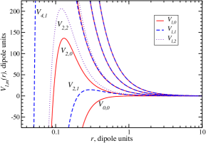
(a) (b)

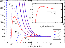
Figure 1: (Color online) Adiabatic potential curves for bosonic (a) and fermionic (b) polar molecules. The curves are labeled by their asymptotic angular momentum $\ell$ and by their exact magnetic quantum number $|m|$. Notice a small potential barrier in the lowest fermionic adiabatic potential $V_{1,0}$.

Neglecting the off-diagonal channel coupling in Eq. (12) yields an adiabatic approximation, in which elementary one-dimensional potentials

$$V_{lm}(r)=\frac{v_{lm}(r)}{r^{2}}+p_{ll}^{(m)}(r)\ \ .$$ (13)

afford a simple, intuitive picture of the scattering. These effective potentials are shown in Fig. 1 for bosonic (a) and fermionic (b) molecules. All the potentials have a very strong short-range attractive well. The long-range behavior in all the channels is $\frac{1}{r^{2}}$, excluding the lowest $V_{0,0}$. This lowest channel is attractive everywhere with a $\frac{1}{r^{4}}$ attractive tail. All the other effective potentials are repulsive at large distances and have a single potential barrier in the transitional region between short-range attraction and long-range repulsion. The barrier heights provide important additional energy scales for the system. As long as the collision energy does not exceed the barrier in the second adiabatic channel, the lowest channel strongly dominates and, therefore determines the character of the dipole-dipole scattering. This serves to identify the ”threshold regime” as corresponding to collision energies that are much smaller than the effective potential barriers. Another important feature of the adiabatic potential curves is the presence of a small, $\sim 0.1$ d.u., barrier in the lowest fermionic channel. This barrier results in substantial differences between fermionic and bosonic threshold scattering.

Contributions of various channels to the total elastic cross-section for bosonic scattering (averaged over the electric-field direction), are shown in Fig. 2 a), for $r_{0}=0.0108$ dipole units. The uncoupled $V_{0,0}$ and $V_{2,1}$ channels dominate bosonic scattering, while $V_{1,0}$ and $V_{1,1}$ dominate fermionic scattering, for energies below $\sim 130E_{D}$, as indicated above. Note, however, that detailed convergence of the cross-section (even at zero energy) requires several adiabatic channels. Both the magnitude of the threshold cross section and the degree of convergence vary with the hard-sphere radius, as they are sensitive to resonance formation in the inner wells of excited potential curves. This is illustrated in Fig. 3, where the elastic cross section (averaged over the field direction) is plotted versus hard-sphere radius at the near-threshold energy, $E=5\times 10^{-4}~{}E_{D}$. Also note that the threshold cross-section varies by 4-orders of magnitude, depending on the specific details of the short-range scattering.

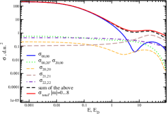
a)	b)
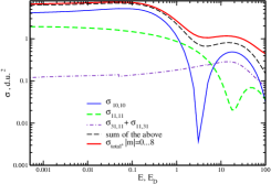
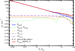
c)	d)

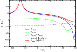
Figure 2: Energy dependence of the field-averaged scattering cross section. a) Bosonic off-resonance scattering, $r_{0}=0.108$. b) Fermionic off-resonance scattering, $r_{0}=0.035$. c) Bosonic resonant scattering, $r_{0}=0.042873$ d) Fermionic resonant scattering, $r0=0.05693$

The nature of these variations can be understood better after a closer look at Fig. 1. Each of the adiabatic channels has a strong short-range attractive core which can support many bound states. When varying the short-range boundary conditions we effectively vary the number of bound states supported by each of the potentials. Each time one of the adiabatic potentials looses a threshold bound state we see a strong variation in the total cross section.

Figure 2 therefore illustrates four distinct cases, depending on the presence of a near-threshold bound state and the system parity. The effect of a near-threshold resonance on the cross section energy dependence is different for bosons and fermions. Even though the threshold bound state strongly influences the magnitude of the cross section in the bosonic case, the energy dependence of the cross section remains qualitatively the same (Fig 2a,c). In the case of fermions, however, there is a striking difference between resonant and off-resonant cases (Fig 2b,d): the shape resonance formed in the lowest adiabatic potential is narrow enough to produce a rapid variation of the cross section. In the non-resonant fermionic case (Fig 2b), when the collision energy approaches the barrier top of $\sim 0.1$d.u. the scattering cross section also grows, although not producing as distinctive a feature as in the resonant scenario (Fig 2d). While bosonic threshold bound states produce a cross section enhancement in a broad range of the cut-off radii $r_{0}$, fermionic cross sections are strongly enhanced only in very close vicinity of the resonant conditions (i.e. the resonances are clearly narrower).

The influence of the short-range cut-off radius on the resonances’ formation can be understood from simple semiclassical analysis, as discussed below.

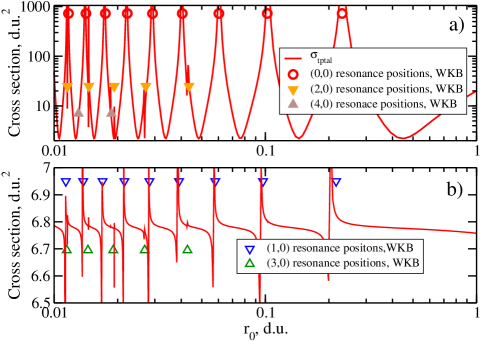
Figure 3: Near-threshold cross section as a function of the cut-off radius for bosons and fermions. Positions of the different $(l,m)$ resonances predicted from WKB match numerical results.

IV Semiclassical analysis

One of the advantages of the adiabatic representation is that it provides a simple interpretation of the entire set of resonances shown in Fig. 3.

Let us look at the case of bosons first (Fig. 3a). Consider the positions of wide peaks corresponding to a near-threshold bound state forming in the lowest adiabatic channel. Such bound states exist if the Bohr-Sommerfeld quantization condition (at $E=0$) is satisfied

$$\int_{r_{0}}^{\infty}\sqrt{2|V_{0,0}(r)|}dr=n\pi+\phi_{0}\ \ .$$

Although the semiclassical condition is not strictly applicable to the calculation of the position of the rightmost peak in Fig. 3a (since the right turning point in the $V_{0,0}$ channel effectively lies at $r\rightarrow\infty$), we have introduced a single fitting parameter $\phi_{0}=0.0735\pi$ in order to reproduce the position of the rightmost peak correctly. Fitting the potential $V_{0,0}$ as $2r^{3}V_{0,0}\approx-\frac{\alpha^{2}}{r+\beta}$ we get an explicit expression for the values of $r_{0}$ that support a near-threshold bound state

$$r_{0}^{(0,0)}(n)=\frac{4\alpha^{2}}{(4\alpha+\beta(\pi n+\phi_{0}))(\pi n+\phi_{0})}\ \ .$$ (14)

The universal dimensionless parameters $\alpha=0.9586$ and $\beta=0.265$ are obtained from fitting the adiabatic potential curve, and Eq. (14) then gives the positions of the peaks in Fig. 3a up to 3 significant figures.

Similarly, the semiclassical description is useful for understanding positions of other resonances that occur in higher adiabatic channels. All the resonances in the model system can be classified according to the asymptotic behaviour of the effective potential that produces the resonance, i.e. the corresponding $(l,m)$ quantum numbers, and the number of bound states supported by the corresponding channel potential. If nonadiabatic coupling could be neglected, the resonances would have zero-width when approaching threshold because of the large dipole-modified centrifugal barrier in Fig. 1. In fact, they dominantly decay into the lowest $m=0$ adiabatic channel through short-range nonadiabatic coupling and show up as Feshbach resonances in the total elastic cross section. Their positions can be found directly from the usual Bohr-Sommerfeld quantization procedure with no fitting parameters. Although it is more difficult to develop a simple fit to the higher adiabatic potentials, an expression similar to (14) provides an excellent fit to the positions of the other resonances obtained from analyzing the semiclassical picture numerically

$$r_{0}^{(l,m)}(n)=\frac{1}{a_{0}+a_{1}n+a_{2}n^{2}}\ \ .$$ (15)

We have performed such fitting for the dominant channels contributing to the low-energy scattering and the results are presented in Table 3.

Table 3: Fitting parameters for resonant short-range cut-off positions $r_{0}$ for the channels dominating at low energy.

$(l,m)$	$a_{0}$	$a_{1}$	$a_{2}$
Bosons
$(0,0)$	0.2447	3.3817	0.711496
$(2,0)$	8.17602	13.5762	0.622266
$(4,0)$	31.6553	21.2334	0.63889
Fermions
$(1,0)$	0.3635	3.567	0.6844
$(3,0)$	10.873	11.809	0.68644
$(5,0)$	32.579	20.671	0.63113

The case of fermions is very similar to the bosonic one, but the potential barrier in the lowest adiabatic channel makes the overall picture quite different: It makes the resonances formed in the lowest adiabatic channel comparatively narrow in both the energy and cut-off radius domains.

V Scattering anisotropy and threshold resonances.

Unlike central potentials, the threshold scattering of dipoles can be strongly anisotropic even in the case of identical bosons. Although the $(0,0)$ channel strongly dominates scattering at low energies, the degree of this domination depends on short-range boundary conditions. For instance, when the total cross-section is minimal, the $(0,0)$ channel does not contribute to scattering, and we can expect the cross section to be strongly anisotropic. This is illustrated in Fig. (4b). At the minimum of the total cross section in the vicinity of the $(2,0)$ resonance (Fig. 4a) the isotropic component of the cross section practically vanishes, and we observe a strong anisotropy both in total cross section i (as a function of the incoming wave direction $\theta$) and in differential cross section (as a function of the incoming wave direction and the scattering angle). In the resonant case, however, when the total cross section is maximal (Fig. 4d), both total and differential cross sections become essentially isotropic with strong domination of the $(0,0)$ channel (s-wave scattering).

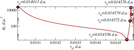
$\sigma$	$d\sigma(\hat{k})$, $\theta=0$	$d\sigma(\hat{k})$, $\theta=\pi/2$	$d\sigma(\hat{k})$, $\cos^{2}\theta=1/3$
b) $r_{0}=0.014556$
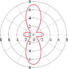
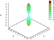
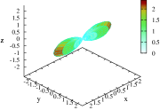
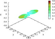
c) $r_{0}=0.014572$
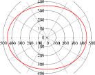
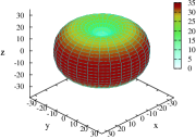
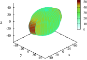
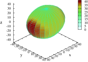
d) $r_{0}=0.014576$
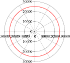
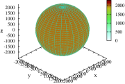
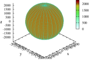
e) $r_{0}=0.014579$

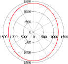
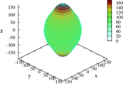
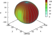
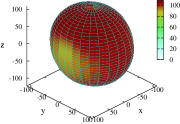
Figure 4: a) Total cross section for two bosons averaged over field direction in the vicinity of the $(0,0)$ (diamond) and $(2,0)$ (circles) resonances. b)-e) Total and differential cross section dependence on the angle $\theta=\cos^{-1}\hat{k}\cdot\hat{z}$ between the incoming wave and the field direction for bosons. Both the total cross section and the differential cross section demonstrate strong dependency on the short-range physics. The dipoles are polarized along the $\hat{z}$ direction, $xz$ defines the scattering plane.

A similar situation occurs for fermions. The angular distribution (which is always anisotropic) is dominated by the rapidly varying $(1,0)$ adiabatic channel, and the rest of the channels that are not that sensitive to the short-range physics. As in the case of bosons, we observe a rapid variation of the angular distributions in the vicinity of a $(3,0)$ resonance (Fig. 5). An interesting feature of the fermionic scattering, however, is the presence of a special direction $\theta=\pi/2$, i.e. collisions perpendicular to the field. Since the contribution of the $(1,0)$ component vanishes in this special direction, scattering perpendicular to the polarizing field is not sensitive to the details of the short-range interaction.

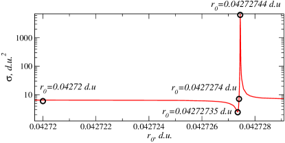
$\sigma$	$d\sigma(\hat{k})$, $\theta=0$	$d\sigma(\hat{k})$, $\theta=\pi/2$	$d\sigma(\hat{k})$, $\cos^{2}\theta=1/3$
b) $r_{0}=0.04272$
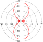
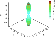
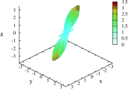
c) $r_{0}=0.04272735$
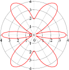
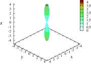
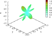
d) $r_{0}=0.0427274$
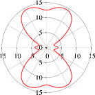
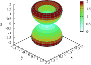
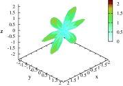
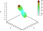
e) $r_{0}=0.0427444$

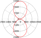
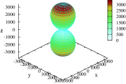
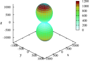
Figure 5: Total and differential cross section dependence on the angle $\theta=\cos^{-1}\hat{k}\cdot\hat{z}$ between the incoming wave and the field direction for fermions. Both the total cross section and the differential cross section demonstrate strong dependency on the short-range physics. Scattering perpendicular to the field is not sensitive to the short-range conditions, however.

VI Some observability notes

Sensitivity to $r_{0}$ indicates a corresponding sensitivity to short-range physics, and therefore, for a given electric field, to the specific molecular species, and some molecules can be expected to be dominated by either resonant or non-resonant adiabatic channels. The dipole moment induced by an external electric field, however, varies with the field until the dipoles are completely polarized. This makes it possible to observe, in principle, the series of resonances which we described in previous section.

Assuming the electric field is large enough to polarize the molecule, but small enough not to perturb the short-range wave function, the only part of the intermolecule interaction affected by the field would be the dipole-dipole interaction. Changing the induced dipole $\mu$ by tuning the electric field we can effectively manage the dipole scales. The elastic scattering cross section $\sigma$ will, therefore, scale with the field ${\cal E}$ as

$$\sigma=D({\cal E})^{2}\sigma(E/E_{D}({\cal E}))$$

where $D({\cal E})$ and $E_{D}({\cal E})$ are given by Eq. 6. As aforementioned, the explicit dependence of the induced dipole moment on the field ${\cal E}$ depends on the molecular state.

As soon as the induced dipole becomes big enough for the dipole length to exceed the short-range scale about 7 times ($R_{0}/D\approx 0.14$), the first bound state is formed in the $V_{0,0}$ potential and the scattering cross section peaks. This is the first peak in the series (14). This first peak would allow an experimentalist to identify the unknown empirical parameter $R_{0}$ and estimate positions of the subsequent peaks of the series (14) from the condition $r_{0}^{(0,0)}(1)=\frac{R_{0}}{D({\cal E})}$. The number of peaks that can be potentially observed for particular molecular species is limited by their intrinsic dipole moment: as $\mu\leq d$, there is a maximal possible dipole scale $D_{max}$, and, thus, the number of peaks $n_{max}$ can be estimated from the condition $r_{0}^{(l,0)}(n_{max})\geq\frac{R_{0}}{D_{max}}$.

Using the parameters for ^6,7LiF molecules given in Table LABEL:Tab:SigmaMol as an example and deliberately choosing $R_{0}=80$ a.u. as a short-range cutoff parameter, we show the direction-averaged total cross section as a function of the external polarizing field in Fig. 6. For weak fields the induced dipole moment is small and, thus, the dipole units are comparable to the short-range molecular scale.

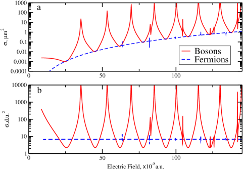
Figure 6: Electric field dependence of the near-threshold ^6,7LiF elastic scattering cross section, in both (a) absolute and (b) dipole units. The minima of the cross section in the upper figure rise rapidly with the field as a result of rapidly growing dipole length. The fermionic cross section exhibits much narrower resonant variations of the cross section while demonstrating the same ${\cal E}^{4}$ growing trend.

Another interesting and universal feature of the dipole-dipole scattering cross section as a function of electric field is the trend of going up with the field. This trend can be seen much more clearly in the case of fermions which exhibits much narrower resonant variations of the cross section.

VII Summary

An adiabatic representation is shown to be useful in numerical calculations of the ultra-low energy dipole-dipole scattering as well as for the classification of resonances that emerge in such systems. For both bose and fermi collision partners, the major resonant phenomena are determined by the $m=0$ channels, especially the lowest channel in the $m=0$ set. The resonant states formed result from the long-range part of the dipole-dipole interaction but are sensitive to interactions that take place at shorter scales. The contribution of short-range interaction can be modulated by tuning the applied field, making it possible to observe a series of resonances. The angular distributions of scattered particles, at ultracold energies, depend sensitively on the resonance positions, and display variable degrees of anisotropy. We have also identified a special scattering direction in the fermionic case that is not sensitive to the short-range physics of the scattered system.

References

- (1) Brian C. Sawyer, Benjamin K. Stuhl, Dajun Wang, Mark Yeo and Jun Ye Preprint arXiv:0806.2624v1 [physics.atom-ph]
- (2) Eric R. Hudson, J.R. Bochinski, H.J. Lewandowski, Brian C. Sawyer, and Jun Ye Eur. Phys. J. D 31, 351–358 (2004)
- (3) S. Ospelkaus, A. Pe’er, K.-K. Ni, J. J. Zirbel, B. Neyenhuis, S. Kotochigova, P. S. Julienne, J. Ye and D. S. Jin Nature Physics 4, 622 - 626 (2008)
- (4) J. Doyle, B. Friedrich, R. V. Krems, and F. Masnou-Seeuws Eur. Phys. J. D 31, 149 (2004)
- (5) Marinescu and L. You, Phys. Rev. Lett. 81, 4596 (1998)
- (6) L. Santos, G. V. Shlyapnikov, P. Zoller and M.Lewenstein Phys. Rev. Lett. 85, 1791 (2000)
- (7) C. Ticknor Phys. Rev. Lett. 100, 133202 (2008)
- (8) C. Ticknor Phys. Rev. A 76, 052703 (2007) (2008)
- (9) C. Ticknor and J. Bohn Phys. Rev. A 72, 032717 (2005)
- (10) J. Bohn and C. Ticknor, in Proceedings of the XVII International Conference on Laser Spectroscopy, E. A. Hinds, A. Ferguson, E. Riis, eds., (World Scientific, 2005), p. 207.
- (11) K. Kanjilal and D. Blume, Preprint arXiv:0806.3991
- (12) V. Roudnev and Mike Cavagnero, Preprint arXiv:0806.1982v2 [physics.atom-ph]
- (13) Alexandr V. Avdeenkov and John L. Bohn, Phys. Rev. A 66, 052718 2002
- (14) Bo Gao, J. Phys. B: At. Mol. Opt. Phys. 37, L227 (2004)
- (15) C. de Boor,B. Swartz, SIAM J. Numer. Anal., 10, 582-606 (1973)
- (16) Frank J. Lovas, Eberhard Tiemann, J. S. Coursey, S. A. Kotochigova, J. Chang, K. Olsen and R. A. Dragoset Diatomic Spectral Database http://physics.nist.gov/PhysRefData/MolSpec/Diatomic/index.html