Recent Developments in the Casimir Effect

Abstract

In this talk I review various developments in the past year concerning quantum vacuum energy, the Casimir effect. In particular, there has been continuing controversy surrounding the temperature correction to the Lifshitz formula for the Casimir force between real materials, be they metals or semiconductors. Consensus has emerged as to how Casimir energy accelerates in a weak gravitational field; quantum vacuum energy, including the divergent parts which renormalize the masses of the Casimir plates, accelerates indeed according to the equivalence principle. Significant development has been forthcoming in applying the multiple scattering formalism to describe the interaction between nontrivial objects. In weak coupling, closed-form expressions for the Casimir force between the bodies, which for example reveal significant discrepancies from the naive proximity force approximation, can be achieved in many cases.

1 Introduction

There has been burgeoning interest in the Casimir effect [1], the quantum force between macroscopic bodies due to zero-point fluctuations, as witnessed by the multitude of international conferences and workshops devoted to the subject, including two in Brazil back-to-back. This interest reflects a great deal of progress in the subject both from the experimental and theoretical sides. I will talk about three topics my collaborators and I have been involved with during the past several months, which mirror these developments: the controversy concerning the temperature dependence of real materials, such as metals and semiconductors; the question of how the Casimir energy associated with parallel Casimir plates is accelerated by gravity; and the achievement of exact closed-form results for the interaction of bodies subject to weak coupling.

2 Temperature Controversy

2.1 Introduction

There is a continuing controversy surrounding the question of how to incorporate thermal corrections into the Casimir force between real metal plates [2, 3]. The procedure to do this seems straightforward. The thermal Green’s functions must be periodic in imaginary time, with period $\beta=1/T$. This implies a Fourier series decomposition, rather than a Fourier transform, where we have a sum over Matsubara frequencies $\zeta_{m}=2\pi mT$.

Thus, the Casimir (Lifshitz) [4] pressure between parallel semi-infinite nonmetallic plates separated by a distance $a$ is given by

$$P^{T}=-\frac{T}{\pi}\sum_{i={\rm TE,TM}}\sum_{m=0}^{\infty}{}^{\prime}\int_{\zeta_{m}}^{\infty}\rmd\kappa\,\kappa^{2}\frac{1}{(r^{i})^{-2}\rme^{2\kappa a}-1},$$ (1)

where the prime means that the $m=0$ term is counted with half weight, in terms of the reflection coefficients

$$r^{\rm TE}=\frac{-\sqrt{1+\frac{\zeta^{2}}{\kappa^{2}}(\varepsilon(\rmi\zeta)-1)}+1}{\sqrt{1+\frac{\zeta^{2}}{\kappa^{2}}(\varepsilon(\rmi\zeta)-1)}+1},$$ (2)

$$r^{\rm TM}=\frac{-\sqrt{1+\frac{\zeta^{2}}{\kappa^{2}}(\varepsilon(\rmi\zeta)-1)}+\varepsilon(\rmi\zeta)}{\sqrt{1+\frac{\zeta^{2}}{\kappa^{2}}(\varepsilon(\rmi\zeta)-1)}+\varepsilon(\rmi\zeta)}.$$ (3)

Let us rewrite the Lifshitz formula at finite temperature in the form

$$P^{T}=\sum_{m=0}^{\infty}{}^{\prime}f_{m}=\int_{0}^{\infty}\rmd m\,f(m)-\sum_{k=0}^{\infty}\frac{B_{2k}}{(2k)!}f^{(2k-1)}(0),$$ (4)

where the second equality uses the Euler-Maclaurin sum formula, in terms of

$$f(m)=-\frac{1}{2\pi\beta}\sum_{i}\int_{0}^{\infty}\rmd k_{\perp}^{2}\,\kappa(\zeta_{m})(d^{i}_{m})^{-1},$$ (5)

where

$$d_{m}^{i}=(r^{i})^{-2}\rme^{2\kappa a}-1,$$ (6)

and $\kappa^{2}=k_{\perp}^{2}+\zeta^{2}$.

Evidently, for the Drude model, where the permittivity has the form

$$\varepsilon(\rmi\zeta)=1+\frac{\omega_{p}^{2}}{\zeta(\zeta+\gamma)},$$ (7)

or more generally, whenever

$$\lim_{\zeta\to 0}\zeta^{2}[\varepsilon(\rmi\zeta)-1]=0,$$ (8)

the TE zero mode vanishes,

$$f^{({\rm TE})}(0)=0.$$ (9)

This leads to a physical discontinuity in the TE mode, between the $m=0$ and $m=1$ Matsubara frequencies. Naively, this implies an additional linear term in the pressure at low temperatures:

$$P^{T}\sim P^{T=0}+\frac{\zeta(3)}{8\pi a^{3}}T,\qquad aT\ll 1.$$ (10)

Exclusion of the TE zero mode will also reduce the linear temperature dependence expected at high temperatures,

$$P^{T}\sim-\frac{\zeta(3)}{8\pi a^{3}}T,\qquad aT\gg 1,$$ (11)

one-half the usual ideal metal result. This anomaly was first pointed out by Boström and Sernelius [5]. See also [6].

Several other recent papers also lend support to our point of view. Jancovici and Šamaj [7, 8] and Buenzli and Martin [9, 10] have examined the Casimir force between ideal-conductor walls with emphasis on the high-temperature limit. Not surprisingly, ideal inert boundary conditions are shown to be inadequate, and fluctuations within the walls, modeled by the classical Debye-Hückel theory, determine the high temperature behavior. The linear in temperature behavior of the Casimir force is found to be reduced by a factor of two from the behavior predicted by an ideal metal, just as seen above in hightlinear. This is precisely the signal of the omission of the $m=0$ TE mode. Further support for our conclusions can be found in the work of Sernelius [11], who calculated the van der Waals-Casimir force between gold plates using the Lindhard or random phase approximation dielectric function. The central theme of his work is to describe the thermal Casimir effect in terms of spatial dispersion. He also finds that for large separations the force is one-half that of the ideal metal. Sernelius shows that, for arbitrary separation between the plates, the spatial-dispersion results nearly exactly coincide with the local dissipation-based results.

Thus, it is very hard to see how the corresponding modification of the low-temperature behavior can be avoided. However, because a linear $T$ dependence in the pressure implies a linear $T$ dependence in the free energy, this seems to imply a violation of the Nernst heat theorem, the third law of thermodynamics, because then a naive calculation implies $S(T=0)\neq 0$. However, we [12] and others have shown that for real metals, where $\gamma$ has a residual value at zero temperature, the free energy per area has a vanishing slope at the origin. Indeed, in the Drude model, the free energy per area has the behavior [13, 14]

$$F=F_{0}+T^{2}\frac{\omega_{p}^{2}}{48\gamma}(2\ln 2-1),$$ (12)

for sufficiently low temperatures. The $T^{5/2}$ and $T^{3}$ corrections to this were calculated last year in [13, 12] This is illustrated in fig_F(T), taken from [12], which shows the numerical evaluation of the free energy for gold.

Figure 1: Numerical evaluation of the free energy between two gold halfspaces as a function of temperature. The inset gives details for low $T$.

2.2 Experimental constraints

The difficulty is that, experimentally, it is not easy to perform Casimir force measurements at other than room temperature, so current constraints on the theory all come from room temperature experiments. Then all one can do is compare the theory at room temperature with the experimental results, which must be corrected for a variety of effects, such as surface roughness, finite conductivity, and patch potentials. There are no direct experiments which observe $T$ dependence in metals! (The temperature dependence of the Casimir-Polder force between a Bose-Einstein condensate and a dielectric substrate was measured in 2006 [15].)

Although the earlier experiment by Lamoreaux [16] was carried out at such large distances ($\sim 1\,\mu$m) where the temperature correction proposed here would be large ($\sim 15$%) [17]. there are reasons to think that the uncertainties due to such things as surface roughness and patch potentials were so large as to afford only limited accuracy in his experiment. There has been a great number of high quality experiments during the last decade, revealing a number of facets of the quantum vacuum energy [18, 19, 20, 21, 22, 23, 24, 25, 26, 27]. As for the temperature effect, the most stringent test is given by the precision experiments of Decca et al.[28, 29], where the agreement of the data with the zero-temperature theory seems to rule out a large thermal correction such as Boström and Sernelius [5] and we have proposed. It seems to us that there may be a number of effects that have not been properly accounted for before one can conclude that no large temperature effect is present, such as the shielding effect recently proposed by Pitaevskii [30].

2.3 Anomaly for semiconductors

Recently Klimchitskaya, Geyer and Mostepanenko [31, 32, 33, 34] have observed there is a similar anomaly, now affecting the TM reflection coefficient, for dielectrics and semiconductors. Here is a simple way to understand that argument. Suppose we model a dielectric with some small conductivity by the permittivity function

$$\varepsilon(i\zeta)=1+\frac{\bar{\varepsilon}-1}{1+\zeta^{2}/\omega_{0}^{2}}+\frac{4\pi\sigma}{\zeta}.$$ (13)

(The only essential point is that as $\zeta\to 0$, $\varepsilon\to\bar{\varepsilon}$ if $\sigma=0$, otherwise $\varepsilon\to\infty$.)

For a dielectric the TE reflection coefficient is continuous, but if there is vanishingly small (but not zero) conductivity the TM coefficient is discontinuous:

$$r^{\rm TM}(\zeta=0)=1,\quad\lim_{\zeta\to 0}r^{\rm TM}=\frac{\bar{\varepsilon}-1}{\bar{\varepsilon}+1}.$$ (14)

This implies a linear term in the pressure

$$P_{T}^{\rm TM} = \frac{T}{2\pi}\int_{0}^{\infty}\rmd\kappa\,\kappa^{2}\left[\frac{1}{\left(\frac{\bar{\varepsilon}+1}{\bar{\varepsilon}-1}\right)^{2}\rme^{2\kappa a}-1}-\frac{1}{\rme^{2\kappa a}-1}\right]$$ (15)

$$= \frac{T}{2\pi}\sum_{n=1}^{\infty}\left[\left(\frac{\bar{\varepsilon}-1}{\bar{\varepsilon}+1}\right)^{2n}-1\right]\int_{0}^{\infty}\rmd\kappa\,\kappa^{2}\rme^{-2n\kappa a}=\frac{T}{8\pi a^{3}}\left[{\rm Li}_{3}\left(\left[\frac{\bar{\varepsilon}-1}{\bar{\varepsilon}+1}\right]^{2}\right)-\zeta(3)\right],$$

where the polylogarithmic function is

$${\rm Li}_{n}(\xi)=\sum_{k=1}^{\infty}\frac{\xi^{k}}{k^{n}}.$$ (16)

Note that the linear term vanishes for $\bar{\varepsilon}\to\infty$. The free energy term $F$ is obtained from this by multiplying by $a/2$. Thus at zero temperature, the entropy is nonzero,

$$S(0)=-\left(\frac{\partial F}{\partial T}\right)_{V}=-\frac{1}{16\pi a^{2}}\left[\mbox{Li}_{3}\left(\left[\frac{\bar{\varepsilon}-1}{\bar{\varepsilon}+1}\right]^{2}\right)-\zeta(3)\right].$$ (17)

Moreover, besides this thermodynamical contradiction, recent experiments by Mohideen’s group [27, 35, 36, 37] show that apparently the conductivity effect must be excluded for semiconductors with very low carrier concentrations, but included for semiconductors with high carrier concentrations. This conundrum has not yet been resolved, although there has been some progress in understanding what happens when the conductivity remains small but nonzero at zero temperature [38] —see also Simen Ådnøy Ellingsen’s talk in this meeting [39]. We should also mention our joint work on temperature effects and anomalies [40] which, while not addressing the semiconductor anomaly, attempts to survey the underpinnings of thermal effects in the Casimir effect.

3 How Does Casimir Energy Fall?

In a series of papers last year [41, 42, 43] we showed that the total Casimir energy of an apparatus consisting of parallel plates, including the divergent parts of the energy, which renormalize the masses of the plates, possesses the gravitational mass demanded by the equivalence principle.

This result puts the lie to the naive presumption that zero-point energy is not observable. On the other hand, because of the severe divergence structure of the theory, controversy has surrounded it from the beginning. Sharp boundaries give rise to divergences in the local energy density near the surface, which may make it impossible to extract meaningful self-energies of single objects, such as the perfectly conducting sphere considered by Boyer [44]. These objections have recently been most forcefully presented by Graham, Jaffe, et al.[45], but they date back to Deutsch and Candelas [46]. In fact, it now appears that these surface divergences can be dealt with successfully in a process of renormalization, and that finite self-energies in the sense of Boyer may be extracted [47, 48].

Gravity couples to the local energy-momentum tensor, and such surface divergences promise serious difficulties. We first ask how does the completely finite Casimir interaction energy of a pair of parallel conducting plates, as well as the divergent self-energies of non-ideal plates, couple to gravity? Disparate answers had been given in the past [49, 50]; thus, the question, and its answer, turn out to be surprisingly less straightforward than the reader might suspect!

We will not here address what gravitational field results from the (in general divergent) Casimir energy. For a beginning of the renormalization of Einstein’s equations resulting from singular Casimir surface energy densities see [51].

Brown and Maclay [52] showed that, for parallel perfectly conducting plates separated by a distance $a$ in the $z$-direction, the electromagnetic stress tensor acquires the vacuum expectation value between the plates

$$\langle T^{\mu\nu}\rangle=\frac{\mathcal{E}_{c}}{a}\mbox{diag}(1,-1,-1,3),\qquad\mathcal{E}_{c}=-\frac{\pi^{2}}{720a^{3}}\hbar c.$$ (18)

Outside the plates the value of $\langle T^{\mu\nu}\rangle=0$.

Because there are some subtleties here, let us review the derivation of t for the case of a conformally coupled scalar (the electromagnetic case differs by a factor of two). Actually, the result between the plates, $0<z<a$, is given in great detail in [53] ($\xi$ is the conformal parameter)

$$\langle T^{\mu\nu}\rangle=(u_{0}+u)\mbox{diag}(1,-1,-1,3)+(1-6\xi)s(z)\mbox{diag}(1,-1,-1,0),$$ (19)

where

$$u_{0}=-\frac{1}{12\pi^{2}}\int_{0}^{\infty}\rmd\kappa\,\kappa^{3},\qquad u=-\frac{\pi^{2}}{1440a^{4}},$$ (20)

Note that $u_{0}$ is a divergent constant, independent of $a$, and is present (as we shall see) both inside and outside the plates, so it does not contribute to any observable force or energy (the force on the plates is given by the discontinuity of $\langle T_{zz}\rangle$), and so may be simply disregarded (as long as we are not concerned with dark energy). Similarly, in terms of the Hurwitz zeta function,

$$s(z)=-\frac{1}{16\pi^{2}a^{4}}[\zeta(4,z/a)+\zeta(4,1-z/a)],$$ (21)

which exhibits the universal surface divergence near the plates,

$$s(z)\sim-\frac{1}{16\pi^{2}z^{4}},\qquad z\to 0+,$$ (22)

is also unobservable (if we disregard gravity) because it does not contribute to the force on the plates, nor does it contribute to the total energy, since the integral over $s(z)$ between the plates is independent of the plate separation. Of course, the best way to eliminate that term is to choose the conformal value $\xi=1/6$.

Since the exterior calculation does not appear to be referred to in [53], let us sketch the calculation here: Consider parallel Dirichlet plates at $z=0$ and $z=a$. The reduced Green’s function satisfies

$$\left(-\frac{\rmd^{2}}{\rmd z^{2}}+\kappa^{2}\right)g(z,z^{\prime})=\delta(z-z^{\prime}),$$ (23)

where $\kappa^{2}=k^{2}-\omega^{2}=k^{2}+\zeta^{2}$. The solution for $z,z^{\prime}<0$ is

$$g(z,z^{\prime})=-\frac{1}{\kappa}e^{\kappa z_{<}}\sinh\kappa z_{>}.$$ (24)

where $z_{<,>}$ means the lesser or greater of $z$ and $z^{\prime}$. It is very straightforward to calculate the one-loop expectation value of the stress tensor from

$$\langle T^{\mu\nu}\rangle=\left(\partial^{\mu}\partial^{\prime\nu}-\frac{1}{2}g^{\mu\nu}\partial^{\lambda}\partial_{\lambda}^{\prime}\right)\frac{1}{\rmi}G(x,x^{\prime})\bigg{|}_{x^{\prime}=x}-\xi(\partial^{\mu}\partial^{\nu}-g^{\mu\nu}\partial^{2})\frac{1}{\rmi}G(x,x),$$ (25)

which follows from

$$\langle\phi(x)\phi(x^{\prime})\rangle=\frac{1}{\rmi}G(x,x^{\prime}).$$ (26)

After integrating over $\omega=\rmi\zeta$ and $\mathbf{k}$, we find the result ($z<0$)

$$\langle T^{\mu\nu}\rangle=u_{0}\mbox{diag}(1,-1,-1,3)-\frac{(1-6\xi)}{16\pi^{2}|z|^{4}}\mbox{diag}(1,-1,-1,0).$$ (27)

This is exactly as expected. The $u_{0}$ term is the same as inside the box, so is just the vacuum value, and the second term is the universal surface divergence seen in indiv (independent of plate separation), which can be eliminated by setting $\xi=1/6$.

Thus, we conclude that the physical stress tensor VEV is just that found by Brown and Maclay [52]:

$$\langle T^{\mu\nu}\rangle=u\,\mbox{diag}(1,-1,-1,3)\theta(z)\theta(a-z).$$ (28)

in terms of the usual step function.

3.1 Variational principle

Now we turn to the question of the gravitational interaction of this Casimir apparatus. It seems this question can be most simply addressed through use of the gravitational definition of the energy-momentum tensor,

$$\delta W_{m}\equiv-\frac{1}{2}\int(\rmd x)\sqrt{-g}\,\delta g^{\mu\nu}T_{\mu\nu}=\frac{1}{2}\int(\rmd x)\sqrt{-g}\,\delta g_{\mu\nu}T^{\mu\nu}.$$ (29)

For a weak field,

$$g_{\mu\nu}=\eta_{\mu\nu}+2h_{\mu\nu},$$ (30)

so if we think of turning on the gravitational field as the perturbation, we can ignore $\sqrt{-g}$. The gravitational energy, for a static situation, is therefore given by ($\delta W=-\int\rmd t\,\delta E$)

$$E_{g}=-\int(\rmd\mathbf{x})h_{\mu\nu}T^{\mu\nu}.$$ (31)

Here we use the gravity-free electromagnetic Casimir stress tensor gravfree, with $u$ now replaced by $\mathcal{E}_{c}/a$ for the electromagnetic situation.

The Fermi metric describes an inertial coordinate system, as we will discuss further below in sec3.2:

$$h_{00}=-gz,\quad h_{0i}=h_{ij}=0.$$ (32)

Let us consider a Casimir apparatus of parallel plates separated by a distance $a$, with transverse dimensions $L\gg a$. Let the apparatus be oriented at an angle $\alpha$ with respect to the direction of gravity, as shown in fig1. The Cartesian coordinate system attached to the earth is $(x,y,z)$, where $z$ is the direction of $-\mathbf{g}$. The Cartesian coordinates associated with the Casimir apparatus are $(\zeta,\eta,\chi)$, where $\zeta$ is normal to the plates, and $\eta$ and $\chi$ are parallel to the plates.

Figure 2: Relation between two Cartesian coordinate frames: One attached to the earth $(x,y,z)$, where $-z$ is the direction of gravity, and one attached to the parallel-plate Casimir apparatus $(\zeta,\eta,\chi)$, where $\zeta$ is in the direction normal to the plates. The parallel plates are indicated by the heavy lines parallel to the $\eta$ axis. The $x=\chi$ axis is perpendicular to the page.

The relation between the two sets of coordinates is

$$z = \zeta\cos\alpha+\eta\sin\alpha,$$ (33)

$$y = \eta\cos\alpha-\zeta\sin\alpha,$$ (34)

$$x = \chi.$$ (35)

Let the center of the apparatus be located at

$$(\zeta=\zeta_{0},\eta=0,\chi=0).$$ (36)

Now we calculate the gravitational energy from ge,

$$E_{g}=\int(\rmd\mathbf{x})gz\langle T^{00}\rangle=\frac{\mathcal{E}_{c}}{a}gL\int_{-L/2}^{L/2}\rmd\eta\int_{\zeta_{0}-a/2}^{\zeta_{0}+a/2}\rmd\zeta(\zeta\cos\alpha+\eta\sin\alpha)\\ =g\mathcal{E}_{c}L^{2}\zeta_{0}\cos\alpha+K,$$

where $K$ is a constant, independent of the center of the apparatus $\zeta_{0}$, $z_{0}=\zeta_{0}\cos\alpha$. Thus, the gravitational force per area $A=L^{2}$ on the apparatus is independent of orientation

$$\mathcal{F}=\frac{F}{A}=-\frac{\partial E_{g}}{A\partial z_{0}}=-g\mathcal{E}_{c}=\epsilon\mathcal{F}_{c},$$ (37)

a small upward push. Here $\epsilon=\frac{1}{3}ga$ is a measure of the gravitational force relative to the Casimir force $\mathcal{F}_{c}=-\pi^{2}/(240a^{4})$. Note that on the earth’s surface, the dimensionless number $\epsilon$ is very small. For a plate separation of $1\mu$m,

$$\epsilon=\frac{ga}{3c^{2}}\sim 10^{-22},$$ (38)

so the considerations here would appear to be only of theoretical interest. The effect is far smaller than the Casimir forces between the plates.

It is a bit simpler to use the energy formula ge to calculate the force by considering the variation in the gravitational energy directly, as we illustrate by considering a mass point at the origin:

$$T^{\mu\nu}=m\delta(\mathbf{r})\delta^{\mu 0}\delta^{\nu 0}.$$ (39)

If we displace the particle rigidly upward by an amount $\delta z_{0}$, the change in the metric is $\delta h_{00}=-g\delta z_{0}$. This implies a change in the energy, exactly as expected:

$$\delta E_{g}=-m\left(-g\delta z_{0}\right)=mg\delta z_{0}.$$ (40)

Now we repeat this calculation for the Casimir apparatus. The gravitational force per area on the rigid apparatus is

$$\mathcal{F}=-\frac{\delta\mathcal{E}_{g}}{\delta z_{0}}=-g\mathcal{E}_{c},$$ (41)

again the same result found in f0, which is 1/4 that found by Bimonte et al.[50]. It does, however, agree with one of the results found in the earlier paper by the same collaboration [49], who now completely agree with our calculation [54]. Our result is further completely consistent with the principle of equivalence, and with one result of Jaekel and Reynaud [55].

In electrodynamics, one defines the field (the 4-vector potential) by

$$\delta W=\int(\rmd x)\delta J^{\mu}A_{\mu}.$$ (42)

From this, one can compute the force on a charge by considering the displacement of a static charge,

$$J^{\mu}=e\delta^{\mu 0}\delta(\mathbf{r}),$$ (43)

that is,

$$\delta J^{\mu}=e\delta^{\mu 0}\left(-\delta\mathbf{r}\cdot\boldsymbol{\nabla}\right)\delta(\mathbf{r}).$$ (44)

Inserting this in the above and integrating by parts we get

$$\delta W=\int\rmd t\int(\rmd\mathbf{r})e\left(-\boldsymbol{\nabla}A^{0}\right)\cdot\delta\mathbf{r}\,\delta(\mathbf{r}).$$ (45)

Because the electric field is $E^{i}=F^{0i}=\partial^{0}A^{i}-\partial^{i}A^{0},$ and a total derivative on time is irrelevant, we deduce the force on the charge to have the expected form:

$$-\frac{\delta E}{\delta\mathbf{r}}=\mathbf{F}=e\mathbf{E}.$$ (46)

We therefore should be able to proceed similarly with vacuum energy, starting from the definition of the gravitational field

$$\delta W=\int(\rmd x)\delta T^{\mu\nu}h_{\mu\nu}.$$ (47)

Again, check this for the force on a mass point, described by mp, so

$$\delta E_{g}=-\int(\rmd\mathbf{r})m\left(-\delta\mathbf{r}\cdot\boldsymbol{\nabla}\right)\delta(\mathbf{r})h^{00}=-m\delta\mathbf{r}\cdot\boldsymbol{\nabla}h^{00}.$$ (48)

Since $h^{00}=-gz$, we conclude

$$-\frac{\delta E}{\delta\mathbf{r}}=\mathbf{F}=-mg\hat{z}.$$ (49)

For the same constant field the force on a Casimir apparatus is obtained from the change in the energy density

$$\langle T^{00}\rangle=\frac{\mathcal{E}_{c}}{a}\theta(a/2-\zeta+\zeta_{0})\theta(\zeta-\zeta_{0}+a/2),$$ (50)

that is, recalling that $z_{0}=\zeta_{0}\cos\alpha$, we obtain the change of the energy density under a rigid displacement $\delta z_{0}$:

$$\delta\langle T^{00}\rangle=\frac{\mathcal{E}_{c}}{a}\delta z_{0}\frac{1}{\cos\alpha}\left[\delta(\zeta-\zeta_{0}-a/2)-\delta(\zeta-\zeta_{0}+a/2)\right],$$ (51)

which yields the gravitational force, since $h^{00}=-g(\zeta\cos\alpha+\eta\sin\alpha)$,

$$\mathcal{F}=-\frac{\delta E_{g}}{A\delta z_{0}}=\frac{F}{A}=\frac{\mathcal{E}_{c}}{a}\frac{1}{\cos\alpha}h^{00}\bigg{|}_{\zeta=\zeta_{0}-a/2}^{\zeta=\zeta_{0}+a/2}=-g\mathcal{E}_{c}.$$ (52)

3.2 Inertial coordinates

However, one might think that the above metric, while sufficing for massive Newtonian objects, might seem inappropriate for photons, near the surface of the earth. Rather, shouldn’t we use the perturbation of the Schwarzchild metric, for weak fields ($GM/r\ll 1$) either in its original or isotropic form? Doing so would give rise to a different force on the Casimir apparatus. The reason we get different answers in different coordinate systems reflects the fact that our starting point is not gauge invariant. Under a coordinate redefinition, which for weak fields is a gauge transformation of $h_{\mu\nu}$ [56]

$$h_{\mu\nu}\to h_{\mu\nu}+\partial_{\mu}\xi_{\nu}+\partial_{\nu}\xi_{\mu},$$ (53)

where $\xi_{\mu}$ is a vector field, the interaction $W$ is invariant only if the stress tensor is conserved, $\partial_{\mu}T^{\mu\nu}=0.$ Otherwise, there is a change in the action,

$$\Delta W=-2\int(\rmd x)\xi_{\nu}\partial_{\mu}T^{\mu\nu}.$$ (54)

Now in our case (where we make the finite size of the plate explicit, but ignore edge effects because $L\gg a$)

$$T^{\mu\nu}=\frac{\mathcal{E}_{c}}{a}\mbox{diag}(1,-1,-1,3)\theta\left(\zeta-\zeta_{0}+\frac{a}{2}\right)\theta\left(\frac{a}{2}-\zeta+\zeta_{0}\right)$$

$$\times\theta(\eta+L/2)\theta(L/2-\eta)\theta(\chi+L/2)\theta(L/2-\chi).$$ (55)

Thus the nonzero components of $\partial_{\mu}T^{\mu\nu}$ are

$$\partial_{\mu}T^{\mu\zeta} = \frac{3\mathcal{E}_{c}}{a}\left[\delta(\zeta-\zeta_{0}+a/2)-\delta(\zeta-\zeta_{0}-a/2)\right]\theta\dots,$$ (56)

$$\partial_{\mu}T^{\mu\eta} = -\frac{\mathcal{E}_{c}}{a}\left[\delta(\eta+L/2)-\delta(\eta-L/2)\right]\theta\dots,$$ (57)

$$\partial_{\mu}T^{\mu\chi} = -\frac{\mathcal{E}_{c}}{a}\left[\delta(\chi+L/2)-\delta(\chi-L/2)\right]\theta\dots,$$ (58)

where $\theta\dots$ refer to the remaining step functions. Therefore, the change in the energy obtained from $\Delta W$ is

$$\Delta E_{g}=\frac{6\mathcal{E}_{c}}{a}\int\rmd\eta\,\rmd\chi\left[\xi_{\zeta}(\zeta_{0}-a/2,\eta,\chi)-\xi_{\zeta}(\zeta_{0}+a/2,\eta,\chi)\right]$$

$$\mbox{}-\frac{2\mathcal{E}_{c}}{a}\!\int\rmd\zeta\,\rmd\chi\left[\xi_{\eta}(\zeta,-L/2,\chi)-\xi_{\eta}(\zeta,L/2,\chi)\right]$$

$$\mbox{}-\frac{2\mathcal{E}_{c}}{a}\int\rmd\zeta\,\rmd\eta\left[\xi_{\chi}(\zeta,\eta,-L/2)-\xi_{\chi}(\zeta,\eta,L/2)\right].$$ (59)

Since we have demonstrated that the gravitational force on a Casimir apparatus is not a gauge-invariant concept, we must ask if there is any way to extract a physically meaningful result. There seem to be two possible ways to proceed. Either we add another interaction, say a fluid exerting a pressure on the plates, resulting in a total stress tensor that is conserved, or we find a physical basis for believing that one coordinate system is more realistic than another. The former procedure is undoubtedly more physical, but will yield model-dependent results. The latter apparently has a natural solution.

A Fermi coordinate system is the general relativistic generalization of an inertial coordinate frame. Such a system has been given in [57] for a resting observer in the field of a static mass distribution. For our case, where the gravitational potential is $\phi=gz$ (apart from an irrelevant additive constant), we recover the Fermi coordinate metric fm for a gravitating body,

$$\rmd s^{2}=-(1+2gz)\rmd t^{2}+\rmd\mathbf{r}^{2}.$$ (60)

This is a priori obvious, because in this coordinate system, coordinate lengths don’t depend on $z$. The Fermi coordinate system may be immediately derived from the Schwarzchild coordinates, far from the gravitating body (so that $GM/r\ll 1$), by a simple coordinate redefinition.

3.3 Alternative derivation

For an alternative derivation of the force on the Casimir apparatus, we start from the variational definition of the stress tensor var, and consider a general coordinate transformation,

$$x^{\prime\mu}=x^{\mu}+\delta x^{\mu},$$ (61)

so that

$$g^{\prime}_{\mu\nu}(x^{\prime})=g^{\prime}_{\mu\nu}(x)+\partial_{\lambda}g_{\mu\nu}\delta x^{\lambda}=g_{\mu\nu}(x)+\delta g_{\mu\nu}(x),$$ (62)

where

$$\delta g_{\mu\nu}=\delta x^{\lambda}\partial_{\lambda}g_{\mu\nu}+g_{\alpha\nu}\frac{\partial\delta x^{\alpha}}{\partial x^{\mu}}+g_{\mu\beta}\frac{\partial\delta x^{\beta}}{\partial x^{\nu}}.$$ (63)

For a rigid translation, $\delta x^{\lambda}$ is a constant, so only the first term here is present, which gives the result found above in sec:vp. However, if we don’t make this restriction, we obtain

$$\delta W=-\int_{\Omega}(\rmd x)\left[\partial_{\nu}\left(\sqrt{-g}T^{\nu}{}_{\lambda}\right)-\frac{1}{2}\sqrt{-g}T^{\mu\nu}\partial_{\lambda}g_{\mu\nu}\right]\delta x^{\lambda}+\int_{\partial\Omega}\rmd\Sigma_{\nu}\sqrt{-g}T^{\nu}{}_{\lambda}\delta x^{\lambda},$$ (64)

where the surface term results from integration by parts. Again, notice for $\delta x^{\lambda}$ constant, the first and third terms identically cancel. If we take the region $\Omega$ to be all space the surface term vanishes (and therefore so does the first term for a rigid displacement). A simple calculation indeed shows that the surface term cancels.

3.4 Rindler coordinates

Relativistically, uniform acceleration is described by hyperbolic motion

$$t=\xi\sinh\tau,\quad z=\xi\cosh\tau,$$ (65)

which corresponds to the metric

$$\rmd t^{2}-\rmd z^{2}-\rmd x_{\perp}^{2}=\xi^{2}\rmd\tau^{2}-\rmd\xi^{2}-\rmd x_{\perp}^{2}.$$ (66)

The d’Alembertian operator has the following form in Rindler coordinates:

$$-\left(\frac{\partial}{\partial t}\right)^{2}+\left(\frac{\partial}{\partial z}\right)^{2}+\nabla_{\perp}^{2}=-\frac{1}{\xi^{2}}\left(\frac{\partial}{\partial\tau}\right)^{2}+\frac{1}{\xi}\frac{\partial}{\partial\xi}\left(\xi\frac{\partial}{\partial\xi}\right)+\nabla_{\perp}^{2}.$$ (67)

In this subsection, we will consider scalar fields and so-called semitransparent plates, that is, ones described by a $\delta$-function potential

$$V=\lambda\delta(\xi-\xi_{a}),$$ (68)

where $\xi_{a}$ is the position of the plate. For a single semitransparent plate at $\xi_{1}$, the Green’s function can be written as

$$G(x,x^{\prime})=\int\frac{\rmd\omega}{2\pi}\frac{\rmd^{2}k}{(2\pi)^{2}}\rme^{-\rmi\omega(\tau-\tau^{\prime})}\rme^{\rmi\mathbf{k\cdot(r-r^{\prime})_{\perp}}}g(\xi,\xi^{\prime}),$$ (69)

where the reduced Green’s function satisfies

$$\left[-\frac{\omega^{2}}{\xi^{2}}-\frac{1}{\xi}\frac{\partial}{\partial\xi}\left(\xi\frac{\partial}{\partial\xi}\right)+k^{2}+\lambda\delta(\xi-\xi_{1})\right]g=\frac{1}{\xi}\delta(\xi-\xi^{\prime}),$$ (70)

which we recognize as just the semitransparent cylinder problem with $m\to\zeta=-\rmi\omega$ and $\kappa\to k$ [48]. The reduced Green’s function for single plate thus is

$$g(\xi,\xi^{\prime})=I_{\zeta}(k\xi_{<})K_{\zeta}(k\xi_{>})-\frac{\lambda\xi_{1}K_{\zeta}^{2}(k\xi_{1})I_{\zeta}(k\xi)I_{\zeta}(k\xi^{\prime})}{1+\lambda\xi_{1}I_{\zeta}(k\xi_{1})K_{\zeta}(k\xi_{1})},\qquad\xi,\xi^{\prime}<\xi_{1},$$ (71)

$$=I_{\zeta}(k\xi_{<})K_{\zeta}(k\xi_{>})-\frac{\lambda\xi_{1}I_{\zeta}^{2}(k\xi_{1})K_{\zeta}(k\xi)K_{\zeta}(k\xi^{\prime})}{1+\lambda\xi_{1}I_{\zeta}(k\xi_{1})K_{\zeta}(k\xi_{1})},\qquad\xi,\xi^{\prime}>\xi_{1}.$$ (72)

In the limit $\lambda\to\infty$ we recover the well-known Green’s function subject to Dirichlet boundary conditions.

If we use the uniform asymptotic expansion (UAE), based on the limit

$$\xi\to\infty, \quad\xi_{1}\to\infty,\quad\xi-\xi_{1}\mbox{ finite },\quad\zeta=\hat{\zeta}\xi_{1}\to\infty,\quad\hat{\zeta}\mbox{ finite },$$ (73)

we recover the Green’s function for a single plate in Minkowski space,

$$\xi_{1}g(\xi,\xi^{\prime})\to\frac{\rme^{-\kappa|\xi-\xi^{\prime}|}}{2\kappa}-\frac{\lambda}{2\kappa}\frac{\rme^{-\kappa(|\xi-\xi_{1}|+|\xi^{\prime}-\xi_{1}|)}}{\lambda+2\kappa},$$ (74)

where $\kappa=\sqrt{k^{2}+\zeta^{2}}$, $\omega=\rmi\zeta$.

The canonical energy-momentum for a scalar field is given by

$$T_{\mu\nu}=\partial_{\mu}\phi\partial_{\nu}\phi+g_{\mu\nu}\frac{1}{\sqrt{-g}}\mathcal{L},$$ (75)

where the Lagrange density includes the $\delta$-function potential. Using the equations of motion, we find the energy density to be

$$T_{00}=\frac{1}{2}\left(\frac{\partial\phi}{\partial\tau}\right)^{2}-\frac{1}{2}\phi\frac{\partial^{2}}{\partial\tau^{2}}\phi+\frac{\xi}{2}\frac{\partial}{\partial\xi}\left(\phi\xi\frac{\partial}{\partial\xi}\phi\right)+\frac{\xi^{2}}{2}\boldsymbol{\nabla}_{\perp}\cdot(\phi\boldsymbol{\nabla}_{\perp}\phi).$$ (76)

From this and similar expressions for the spatial components of $T^{\mu\nu}$ we can obtain $\langle T_{\mu\nu}\rangle$ by applying a differential operator to the Green’s function, in view of the one-loop connection vev.

The force density is given by

$$f_{\lambda}=-\frac{1}{\sqrt{-g}}\partial_{\nu}(\sqrt{-g}T^{\nu}{}_{\lambda})+\frac{1}{2}T^{\mu\nu}\partial_{\lambda}g_{\mu\nu},$$ (77)

which follows from intbyparts, or

$$f_{\xi}=-\frac{1}{\xi}\partial_{\xi}(\xi T^{\xi\xi})-\xi T^{00}.$$ (78)

When we integrate over all space to get the force,

$$F=\int(\rmd\mathbf{x})\sqrt{-g}f_{\xi},$$ (79)

the first term in fxi is a surface term which does not contribute, as noted in intbyparts, so the gravitational force on the system is

$$\mathcal{F}=\int\rmd\xi\xi f_{\xi}=-\int\frac{\rmd\xi}{\xi^{2}}T_{00},$$ (80)

which when multiplied by the gravitational acceleration $g$ is the gravitational force/area on the Casimir energy. Using the expression t00 for the energy density, and rescaling we see that

$$\mathcal{F}=\int\rmd\xi\xi\int\frac{\rmd\hat{\zeta}\,\rmd^{2}k}{(2\pi)^{3}}\hat{\zeta}^{2}g(\xi,\xi)\quad(\zeta=\hat{\zeta}\xi).$$ (81)

This result is an immediate consequence of the general formula [58]

$$E_{c}=\frac{1}{2\rmi}\int(\rmd\mathbf{r})\int\frac{\rmd\omega}{2\pi}2\omega^{2}\mathcal{G}(\mathbf{r,r}),$$ (82)

in terms of the frequency transform of the Green’s function,

$$G(x,x^{\prime})=\int_{-\infty}^{\infty}\frac{\rmd\omega}{2\pi}\rme^{-i\omega(t-t^{\prime})}\mathcal{G}(\mathbf{r,r^{\prime}}).$$ (83)

Alternatively, we can start from the following formula for the force density for a single semitransparent plate,

$$f_{\xi}=\frac{1}{2}\phi^{2}\partial_{\xi}\lambda\delta(\xi-\xi_{1}),$$ (84)

or, in terms of the Green’s function,

$$\mathcal{F}=-\lambda\frac{1}{2}\int\frac{\rmd\zeta\,\rmd^{2}k}{(2\pi)^{3}}\partial_{\xi_{1}}[\xi_{1}g(\xi_{1},\xi_{1})].$$ (85)

For example, the force on a single plate is given by

$$\mathcal{F}=-\partial_{\xi_{1}}\frac{1}{2}\int\frac{\rmd\zeta\,\rmd^{2}k}{(2\pi)^{3}}\ln[1+\lambda I_{\zeta}(k\xi_{1})K_{\zeta}(k\xi_{1})],$$ (86)

Expanding this about some arbitrary point $\xi_{0}$, with $\zeta=\hat{\zeta}\xi_{0}$, and using the UAE, we get

$$\mathcal{F}=-\frac{1}{96\pi^{2}a^{3}}\int_{0}^{\infty}\frac{\rmd y\,y^{2}}{1+y/\lambda a},$$ (87)

which is just the negative of the (divergent) quantum vacuum energy of a single plate.

For two plates at $\xi_{1}$, $\xi_{2}$, for $\xi,\xi^{\prime}<\xi_{1}<\xi_{2}$,

$$g(\xi,\xi^{\prime})=I_{<}K_{>}-\frac{\lambda_{1}\xi_{1}K_{1}^{2}+\lambda_{2}\xi_{2}K_{1}^{2}-\lambda_{1}\lambda_{2}\xi_{1}\xi_{2}K_{1}K_{2}(K_{2}I_{1}-K_{1}I_{2})}{\Delta}II_{\prime},$$ (88)

while for $\xi,\xi^{\prime}>\xi_{2}>\xi_{1}$,

$$g(\xi,\xi^{\prime})=I_{<}K_{>}-\frac{\lambda_{1}\xi_{1}I_{1}^{2}+\lambda_{2}\xi_{2}I_{2}^{2}+\lambda_{1}\lambda_{2}\xi_{1}\xi_{2}I_{1}I_{2}(I_{2}K_{1}-I_{1}K_{2})}{\Delta}KK_{\prime},$$ (89)

and between the plates, $\xi_{1}<\xi,\xi^{\prime}<\xi_{2}$,

$$g(\xi,\xi^{\prime})=I_{<}K_{>}-\frac{\lambda_{2}\xi_{2}K_{2}^{2}(1+\lambda_{1}\xi_{1}K_{1}I_{1})}{\Delta}II_{\prime}-\frac{\lambda_{1}\xi_{1}I_{1}^{2}(1+\lambda_{2}\xi_{2}K_{1}I_{1})}{\Delta}KK_{\prime}$$

$$\mbox{}+\frac{\lambda_{1}\lambda_{2}\xi_{1}\xi_{2}I_{1}^{2}K_{2}^{2}}{\Delta}(IK_{\prime}+KI_{\prime}),$$ (90)

where

$$\Delta={1+\lambda_{1}\xi_{1}K_{1}I_{1}+\lambda_{2}\xi_{2}I_{2}K_{2}-\lambda_{1}\lambda_{2}\xi_{1}\xi_{2}I_{1}K_{2}(I_{1}K_{2}-I_{2}K_{1})},$$ (91)

and where we have used the abbreviations $I_{a}=I_{\zeta}(k\xi_{a})$, $I=I_{\zeta}(k\xi)$, $I_{\prime}=I_{\zeta}(k\xi^{\prime})$, etc.

In the weak acceleration limit, the Green’s function reduces to exactly the expected result, for $\xi_{1}<\xi,\xi^{\prime}<\xi_{2}$ ($a=\xi_{2}-\xi_{1}$)

$$\xi_{0}g(\xi,\xi^{\prime})\to\frac{1}{2\kappa}\rme^{-\kappa|\xi-\xi^{\prime}|}+\frac{1}{2\kappa\tilde{\Delta}}\bigg{[}\frac{\lambda_{1}\lambda_{2}}{4\kappa^{2}}2\cosh\kappa(\xi-\xi^{\prime})$$

$$\mbox{}-\frac{\lambda_{1}}{2\kappa}\left(1+\frac{\lambda_{2}}{2\kappa}\right)\rme^{-\kappa(\xi+\xi^{\prime}-2\xi_{2})}-\frac{\lambda_{2}}{2\kappa}\left(1+\frac{\lambda_{1}}{2\kappa}\right)\rme^{\kappa(\xi+\xi^{\prime}-2\xi_{1})}\bigg{]},$$ (92)

with

$$\tilde{\Delta}=\left(1+\frac{\lambda_{1}}{2\kappa}\right)\left(1+\frac{\lambda_{2}}{2\kappa}\right)\rme^{2\kappa a}-\frac{\lambda_{1}\lambda_{2}}{4\kappa^{2}},$$ (93)

The flat space limit also holds outside the plates.

In general, we have two alternative forms for the force on the two-plate system:

$$\mathcal{F}=-(\partial_{\xi_{1}}+\partial_{\xi_{2}})\frac{1}{2}\int\frac{\rmd\zeta\,\rmd^{2}k}{(2\pi)^{3}}\ln\Delta,$$ (94)

which is equivalent to genforce. From either of these two formulæ, we find the gravitational force on the Casimir energy to be in the $\xi\to\infty$ limit

$$\mathcal{F}=-\frac{1}{4\pi^{2}}\int_{0}^{\infty}\rmd\kappa\,\kappa^{2}\ln\Delta_{0}$$ (95)

where $\Delta_{0}=\rme^{-2\kappa a}\tilde{\Delta}$, $\tilde{\Delta}$ given in tdelta. From this we get the explicit force

$$\mathcal{F} = \frac{1}{96\pi^{2}a^{3}}\int_{0}^{\infty}\rmd y\,y^{3}\frac{1+\frac{1}{y+\lambda_{1}a}+\frac{1}{y+\lambda_{2}a}}{\left(\frac{y}{\lambda_{1}a}+1\right)\left(\frac{y}{\lambda_{2}a}+1\right)\rme^{y}-1}$$ (96)

$$\mbox{}-\frac{1}{96\pi^{2}a^{3}}\int_{0}^{\infty}\rmd y\,y^{2}\left[\frac{1}{\frac{y}{\lambda_{1}a}+1}+\frac{1}{\frac{y}{\lambda_{2}a}+1}\right]=-(\mathcal{E}_{c}+\mathcal{E}_{d1}+\mathcal{E}_{d2}),$$

which is just the negative of the Casimir energy of the two semitransparent plates, including divergent parts associated with each plate. The divergent terms simply renormalize the masses $m_{i}$ per area of each plate:

$$\mathcal{E}_{\rm total}=m_{1}+m_{2}+\mathcal{E}_{d1}+\mathcal{E}_{d2}+\mathcal{E}_{c}=M_{1}+M_{2}+\mathcal{E}_{c},$$ (97)

$M_{i}=m_{i}+\mathcal{E}_{di}$, and thus the gravitational force on the entire apparatus obeys the equivalence principle

$$g\mathcal{F}=-g(M_{1}+M_{2}+\mathcal{E}_{c}).$$ (98)

3.5 Centripetal Acceleration

Consider finally a Casimir apparatus undergoing centripetal acceleration with angular velocity $\omega$ ($\omega r\ll 1$), as illustrated in figcent1. A detailed calculation [59] shows that the force on the Casimir apparatus is just as expected, including the divergent pieces which renormalize the masses per area $A$ of the plates:

$$\frac{\mathbf{F}}{A}=-\frac{\omega^{2}}{A}\int\rmd^{3}x\,\mathbf{r}\,t^{00}(\mathbf{r})=-\omega^{2}\mathbf{r}_{\rm CM}(m_{1}+m_{2}+\mathcal{E}_{d1}+\mathcal{E}_{d2}+\mathcal{E}_{c}),$$ (99)

where $\mathbf{r}_{\rm CM}$ is the center of energy of the entire system. Nontrivial is the fact that this result is independent of the orientation of the plates.

Figure 3: Casimir apparatus undergoing uniform circular motion with angular velocity $\omega$. The figure on the left has the Casimir plates tangent to the circle of revolution, while on the right the plates make an angle $\alpha$ with respect to that tangent.

4 Multiple Scattering Technique

In the past few years, there has been a tremendous resurgence of interest in the multiple-scattering technique. This is largely inspired by the desire to improve the comparison with experiment, such comparison heretofore having been restricted to the use of the “proximity force approximation,” which describes the Casimir interaction between bodies with curved surfaces by pairwise interactions between small plane elements of the surfaces [60]. The multiple-scattering method certainly dates back to at least the Krein formula [61], and was first used in connection with the Casimir effect by Renne [62]. A most famous variation were the multiple reflection calculations of Balian and Duplantier [63]. In the last few years there has been an explosion of publications on variations of this technique, as physicists realized it could be practically used to obtain numerical results for forces between bodies of arbitrary shapes, for example [64, 65, 66, 67, 68, 69, 70, 71, 72, 73, 74, 75, 76].

We have also contributed to this redevelopment, giving the general formulation for scalar fields [77], and applying it to bodies described by $\delta$-function potentials [78], and, after generalizing to electrodynamics, to dielectric bodies [79]. The methodology has also been applied to non-contact gears [80, 81].

The multiple scattering approach starts from the well-known formula for the vacuum energy or Casimir energy (for simplicity here we first restrict attention to a massless scalar field)($\tau$ is the “infinite” time that the configuration exists)

$$E=\frac{\rmi}{2\tau}\mbox{Tr}\ln G\to\frac{\rmi}{2\tau}\mbox{Tr}\ln GG_{0}^{-1},$$ (100)

where $G$ ($G_{0}$) is the Green’s function,

$$(-\partial^{2}+V)G=1,\quad-\partial^{2}G_{0}=1,$$ (101)

subject to appropriate boundary conditions at infinity. We will use the Feynman or causal Green’s functions.

Now we define the $T$-matrix [82]

$$T=S-1=V(1+G_{0}V)^{-1}.$$ (102)

If the potential has two disjoint parts, $V=V_{1}+V_{2}$ it is easy to derive

$$T=(V_{1}+V_{2})(1-G_{0}T_{1})(1-G_{0}T_{1}G_{0}T_{2})^{-1}(1-G_{0}T_{2}),$$ (103)

where

$$T_{i}=V_{i}(1+G_{0}V_{i})^{-1},\quad i=1,2.$$ (104)

Thus, we can write the general expression for the interaction between the two bodies (potentials) in two equivalent forms:

$$E_{12} = -\frac{\rmi}{2\tau}\mbox{Tr}\ln(1-G_{0}T_{1}G_{0}T_{2})$$ (105)

$$= -\frac{\rmi}{2\tau}\mbox{Tr}\ln(1-V_{1}G_{1}V_{2}G_{2}),$$ (106)

where $G_{i}=(1+G_{0}V_{i})^{-1}G_{0},\quad i=1,2.$

4.1 Multipole expansion

To proceed to apply this method to general bodies, we use an even older technique, the multipole expansion. Let’s illustrate this with a $2+1$ dimensional version, which allows us to describe cylinders with parallel axes. We seek an expansion of the free Green’s function

$$G_{0}(\mathbf{R+r^{\prime}-r})=\frac{\rme^{\rmi|\omega||\mathbf{r-R-r^{\prime}}|}}{4\pi|\mathbf{r-R-r^{\prime}}|}=\int\frac{\rmd k_{z}}{2\pi}\rme^{\rmi k_{z}(z-Z-z^{\prime})}g_{0}(\mathbf{r_{\perp}-R_{\perp}-r^{\prime}_{\perp}}).$$ (107)

Here, the reduced Green’s function is ($\omega=\rmi\zeta$)

$$g_{0}(\mathbf{r_{\perp}-R_{\perp}-r^{\prime}_{\perp}})=\int\frac{(\rmd^{2}k_{\perp})}{(2\pi)^{2}}\frac{\rme^{-\rmi\mathbf{k_{\perp}\cdot R_{\perp}}}\rme^{\rmi\mathbf{k_{\perp}\cdot(r_{\perp}-r^{\prime}_{\perp})}}}{k_{\perp}^{2}+k_{z}^{2}+\zeta^{2}}.$$ (108)

As long as the two potentials do not overlap, so that we have $\mathbf{r_{\perp}-R_{\perp}-r^{\prime}_{\perp}}\neq 0$, we can write an expansion in terms of modified Bessel functions:

$$g_{0}(\mathbf{r_{\perp}-R_{\perp}-r^{\prime}_{\perp}})=\sum_{m,m^{\prime}}I_{m}(\kappa r)\rme^{\rmi m\phi}I_{m}^{\prime}(\kappa r^{\prime})\rme^{-\rmi m^{\prime}\phi^{\prime}}\tilde{g}^{0}_{m,m^{\prime}}(\kappa R),\quad\kappa^{2}=k_{z}^{2}+\zeta^{2}.$$ (109)

By Fourier transforming, and using the definition of the Bessel function

$$\rmi^{m}J_{m}(kr)=\int_{0}^{2\pi}\frac{\rmd\phi}{2\pi}\,\rme^{-\rmi m\phi}\rme^{\rmi kr\cos\phi},$$ (110)

we easily find

$$\tilde{g}^{0}_{m,m^{\prime}}(\kappa R)=\frac{1}{2\pi}\int\frac{\rmd k\,k}{k^{2}+\kappa^{2}}J_{m-m^{\prime}}(kR)\frac{J_{m}(kr)J_{m}(kr^{\prime})}{I_{m}(\kappa r)I_{m}(\kappa r^{\prime})}=\frac{(-1)^{m^{\prime}}}{2\pi}K_{m-m^{\prime}}(\kappa R).$$ (111)

Thus we can derive an expression for the interaction between two bodies, in terms of discrete matrices,

$$\mathfrak{E}\equiv\frac{E_{\rm int}}{L}=\frac{1}{8\pi^{2}}\int\rmd\zeta\,\rmd k_{z}\ln\det\left(1-\tilde{g}^{0}\tilde{T}_{1}\tilde{g}^{0\top}\tilde{T}_{2}\right),$$ (112)

where $\top$ denotes transpose, and the $\tilde{T}$ matrix elements are given by

$$\tilde{T}_{mm^{\prime}}=\int\rmd r\,r\,\rmd\phi\int\rmd r^{\prime}\,r^{\prime}\,\rmd\phi^{\prime}I_{m}(\kappa r)\rme^{-\rmi m\phi}I_{m^{\prime}}(\kappa r^{\prime})\rme^{\rmi m^{\prime}\phi^{\prime}}T(r,\phi;r^{\prime},\phi^{\prime}).$$ (113)

We will apply this 2+1 dimensional formalism to the interaction between two cylinders, as illustrated in pfa. Also illustrated there is the idea behind the proximity force approximation, which applies when the separation between the bodies is much smaller than the radii of curvature of the bodies.

Figure 4: Geometry of two cylinders (or two spheres) with radii $a$ and $b$, respectively, and distances between their centers of $R>a+b$. The proximity force approximation applies when the distance of closest approach $d=R-a-b\ll a,b$. The approximation consists in assuming that the interaction is dominated by the interaction of adjacent surface elements, as shown.

Consider two parallel semitransparent cylinders, of radii $a$ and $b$, respectively, lying outside each other, described by the potentials

$$V_{1}=\lambda_{1}\delta(r-a),\quad V_{2}=\lambda_{2}\delta(r^{\prime}-b),$$ (114)

with the separation between the centers $R$ satisfying $R>a+b$. It is easy to work out the scattering matrix in this situation,

$$(t_{1})_{mm^{\prime}}=2\pi\lambda_{1}a\delta_{mm^{\prime}}\frac{I_{m}^{2}(\kappa a)}{1+\lambda_{1}aI_{m}(\kappa a)K_{m}(\kappa a)}.$$ (115)

Thus the Casimir energy per unit length is

$$\mathfrak{E}=\frac{1}{4\pi}\int_{0}^{\infty}\rmd\kappa\,\kappa\,\mbox{tr}\ln(1-A),$$ (116)

where $A=B(a)B(b)$, in terms of the matrices

$$B_{mm^{\prime}}(a)=K_{m+m^{\prime}}(\kappa R)\frac{\lambda_{1}aI_{m^{\prime}}^{2}(\kappa a)}{1+\lambda_{1}aI_{m^{\prime}}(\kappa a)K_{m^{\prime}}(\kappa a)}.$$ (117)

The strong coupling limit, the case of Dirichlet cylinders, has been considered in [75], for example. In contrast, here we will consider the situation of weak coupling, $\lambda_{1}a\ll 1$, $\lambda_{2}b\ll 1$, where the formula for the interaction energy between two cylinders becomes

$$\mathfrak{E}=-\frac{\lambda_{1}\lambda_{2}ab}{4\pi R^{2}}\sum_{m,m^{\prime}=-\infty}^{\infty}\int_{0}^{\infty}\rmd x\,x\,K_{m+m^{\prime}}^{2}(x)I_{m}^{2}(xa/R)I_{m^{\prime}}^{2}(xb/R).$$ (118)

One merely exploits the small argument expansion for the modified Bessel functions $I_{m}(xa/R)$ and $I_{m^{\prime}}(xb/R)$:

$$I_{m}^{2}(x)=\left(\frac{x}{2}\right)^{2|m|}\sum_{n=0}^{\infty}Z_{|m|,n}\left(\frac{x}{2}\right)^{2n},$$ (119)

where the coefficients $Z_{m,n}$ are

$$Z_{m,n}=\frac{2^{2(m+n)}\;\Gamma\left(m+n+\frac{1}{2}\right)}{\sqrt{\pi}\;n!\;(2m+n)!\;\Gamma(m+n+1)}.$$ (120)

In this case we get an amazingly simple result

$$\mathfrak{E}=-\frac{\lambda_{1}a\lambda_{2}b}{4\pi R^{2}}\frac{1}{2}\sum_{n=0}^{\infty}\left(\frac{a}{R}\right)^{2n}P_{n}(\mu),$$ (121)

where $\mu=b/a$, and where by inspection we identify the binomial coefficients

$$P_{n}(\mu)=\sum_{k=0}^{n}{n\choose{k}}^{2}\mu^{2k}.$$ (122)

Remarkably, it is possible to perform the sums, so we obtain the following closed form for the interaction between two weakly-coupled cylinders:

$$\mathfrak{E}=-\frac{\lambda_{1}a\lambda_{2}b}{8\pi R^{2}}\left[\!\!\left(1-\left(\frac{a+b}{R}\right)^{2}\right)\!\!\left(1-\left(\frac{a-b}{R}\right)^{2}\right)\!\!\right]^{-1/2}.$$ (123)

We note that in the limit $R-a-b=d\to 0$, $d$ being the distance between the closest points on the two cylinders, we recover the proximity force theorem in this case

$$U(d)=-\frac{\lambda_{1}\lambda_{2}}{32\pi}\sqrt{\frac{2ab}{R}}\frac{1}{d^{1/2}},\qquad d\ll a,b.$$ (124)

The rate of approach is given by

$$\frac{\mathfrak{E}}{U}\approx 1-\frac{1+\mu+\mu^{2}}{4\mu}\frac{d}{R}\approx 1-\frac{R^{2}-aR+a^{2}}{4a(R-a)}\frac{d}{R}.$$ (125)

The comparison between the exact result, and the proximity force approximation pfawccyl1 is given in figwccyl1, for equal radii, and in figwccyl2 for unequal radii. Evidently, the proximity force approximation fails badly as the cylinders are pulled apart.

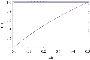
Figure 5: Plotted is the ratio of the exact interaction energy of two equal radii weakly-coupled cylinders to the proximity force approximation.

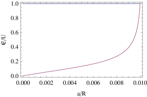
Figure 6: Plotted is the ratio of the exact interaction energy of two weakly-coupled cylinders with ratio of radii $b/a=99$ to the proximity force approximation.

We can similarly consider the interaction between a cylinder and a plane. By the method of images, we can find the interaction between a semitransparent cylinder and a Dirichlet plane to be

$$\mathfrak{E}=\frac{1}{4\pi}\int_{0}^{\infty}\kappa\,\rmd\kappa\,\mbox{tr}\,\ln(1-B(a)),$$ (126)

where $B(a)$ is given in bofa. In the strong-coupling limit this result agrees with that given by Bordag and Nikolaev [72], because

$$\mbox{tr}\,B^{s}=\mbox{tr}\,\tilde{B}^{s},\quad\tilde{B}_{mm^{\prime}}=\frac{1}{K_{m}(\kappa a)}K_{m+m^{\prime}}(\kappa R)I_{m^{\prime}}(\kappa a).$$ (127)

In exactly the way given above, we can obtain a closed-form result for the interaction energy between a Dirichlet plane and a weakly-coupled cylinder of radius $a$ separated by a distance $R/2$. The result is again quite simple:

$$\mathfrak{E}=-\frac{\lambda a}{4\pi R^{2}}\left[1-\left(\frac{2a}{R}\right)^{2}\right]^{-3/2}.$$ (128)

In the limit as $d\to 0$, this agrees with the PFA for this situation:

$$U(d)=-\frac{\lambda}{64\pi}\frac{\sqrt{2a}}{d^{3/2}}.$$ (129)

Note again that this form is ambiguous: the proximity force theorem is equally well satisfied if we replace $a$ by $R/2$, for example, in $U(d)$. The exact result is compared with the PFA in figcylpl.

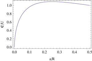
Figure 7: Interaction energy between a weakly coupled $\delta$-function cylinder and a Dirichlet plane. Plotted is the ratio between the energy and the PFA approximation pfa:cylpl.

4.2 3-dimensional formalism

The three-dimensional formalism is very similar. In this case, the free Green’s function has the representation

$$G_{0}(\mathbf{R+r^{\prime}-r}) = \sum_{lm,l^{\prime}m^{\prime}}j_{l}(\rmi|\zeta|r)j_{l^{\prime}}(\rmi|\zeta|r^{\prime})Y_{lm}^{*}(\mathbf{\hat{r}})Y_{l^{\prime}m^{\prime}}(\mathbf{\hat{r}^{\prime}})g_{lm,l^{\prime}m^{\prime}}(\mathbf{R}).$$ (130)

The reduced Green’s function can be written in the form

$$g^{0}_{lm,l^{\prime}m^{\prime}}(\mathbf{R})=(4\pi)^{2}\rmi^{l^{\prime}-l}\int\frac{(\rmd\mathbf{k})}{(2\pi)^{3}}\frac{\rme^{\rmi\mathbf{k\cdot R}}}{k^{2}+\zeta^{2}}\frac{j_{l}(kr)j_{l^{\prime}}(kr^{\prime})}{j_{l}(\rmi|\zeta|r)j_{l^{\prime}}(\rmi|\zeta|r^{\prime})}Y_{lm}(\mathbf{\hat{k}})Y^{*}_{l^{\prime}m^{\prime}}(\mathbf{\hat{k}}).$$ (131)

Now we use the plane-wave expansion

$$\rme^{\rmi\mathbf{k\cdot R}}=4\pi\sum_{l^{\prime\prime}m^{\prime\prime}}\rmi^{l^{\prime\prime}}j_{l^{\prime\prime}}(kR)Y_{l^{\prime\prime}m^{\prime\prime}}(\mathbf{\hat{R}})Y_{l^{\prime\prime}m^{\prime\prime}}^{*}(\mathbf{\hat{k}}),$$ (132)

so now we encounter something new, an integral over three spherical harmonics,

$$\int\rmd\mathbf{\hat{k}}Y_{lm}(\mathbf{\hat{k}})Y_{l^{\prime}m^{\prime}}^{*}(\mathbf{\hat{k}})Y_{l^{\prime\prime}m^{\prime\prime}}^{*}(\mathbf{\hat{k}})=C_{lm,l^{\prime}m^{\prime},l^{\prime\prime}m^{\prime\prime}},$$ (133)

where

$$C_{lm,l^{\prime}m^{\prime},l^{\prime\prime}m^{\prime\prime}}=(-1)^{m^{\prime}+m^{\prime\prime}}\sqrt{\frac{(2l+1)(2l^{\prime}+1)(2l^{\prime\prime}+1)}{4\pi}}\left(\begin{array}[]{ccc}l&l^{\prime}&l^{\prime\prime}\\ 0&0&0\end{array}\right)\left(\begin{array}[]{ccc}l&l^{\prime}&l^{\prime\prime}\\ m&m^{\prime}&m^{\prime\prime}\end{array}\right).$$ (138)

The three-$j$ symbols (Wigner coefficients) here vanish unless $l+l^{\prime}+l^{\prime\prime}$ is even. This fact is crucial, since because of it we can write $j_{l^{\prime\prime}}(kR)$ in terms of Hankel functions of the first and second kind, using the reflection property of the latter,

$$h_{l^{\prime\prime}}^{(2)}(kR)=(-1)^{l^{\prime\prime}}h^{(1)}_{l^{\prime\prime}}(-kR),$$ (139)

and then extending the $k$ integral over the entire real axis to a contour integral closed in the upper half plane. This leads to

$$g^{0}_{lm,l^{\prime}m^{\prime}}(\mathbf{R})=4\pi\rmi^{l^{\prime}-l}\sqrt{\frac{2|\zeta|}{\pi R}}\sum_{l^{\prime\prime}m^{\prime\prime}}C_{lm,l^{\prime}m^{\prime},l^{\prime\prime}m^{\prime\prime}}K_{l^{\prime\prime}+1/2}(|\zeta|R)Y_{l^{\prime\prime}m^{\prime\prime}}(\mathbf{\hat{R}}).$$ (140)

For the case of two semitransparent spheres that are totally outside each other,

$$V_{1}(r)=\lambda_{1}\delta(r-a),\qquad V_{2}(r^{\prime})=\lambda_{2}\delta(r^{\prime}-b),$$ (141)

in terms of spherical coordinates centered on each sphere, it is again very easy to calculate the scattering matrices,

$$T_{1}(\mathbf{r,r^{\prime}})=\frac{\lambda_{1}}{a^{2}}\delta(r-a)\delta(r^{\prime}-a)\sum_{lm}\frac{Y_{lm}(\mathbf{\hat{r}})Y_{lm}^{*}(\mathbf{\hat{r}^{\prime}})}{1+\lambda_{1}aK_{l+1/2}(|\zeta|a)I_{l+1/2}(|\zeta|a)},$$ (142)

and then the harmonic transform is very similar to that seen for the cylinder, ($k=\rmi|\zeta|$)

$$(t_{1})_{lm,l^{\prime}m^{\prime}} = \int(\rmd\mathbf{r})(\rmd\mathbf{r^{\prime}})j_{l}(kr)Y^{*}_{lm}(\mathbf{\hat{r}})j_{l^{\prime}}(kr^{\prime})Y_{l^{\prime}m^{\prime}}(\mathbf{\hat{r}^{\prime}})T_{1}(\mathbf{r,r^{\prime}})$$ (143)

$$= \delta_{ll^{\prime}}\delta_{mm^{\prime}}(-1)^{l}\frac{\lambda_{1}a\pi}{2|\zeta|}\frac{I_{l+1/2}^{2}(|\zeta|a)}{1+\lambda_{1}aK_{l+1/2}(|\zeta|a)I_{l+1/2}(|\zeta|a)}.$$

Let us suppose that the two spheres lie along the $z$-axis, that is, $\mathbf{R}=R\mathbf{\hat{z}}$. Then we can simplify the expression for the energy somewhat by using $Y_{lm}(\theta=0)=\delta_{m0}\sqrt{(2l+1)/4\pi}$. The formula for the energy of interaction becomes

$$E=\frac{1}{2\pi}\int_{0}^{\infty}\rmd\zeta\,\mbox{tr}\ln(1-A),$$ (144)

in terms of the matrix

$$A_{lm,l^{\prime}m^{\prime}}=\delta_{m,m^{\prime}}\sum_{l^{\prime\prime}}B_{ll^{\prime\prime}m}(a)B_{l^{\prime\prime}l^{\prime}m}(b)$$ (145)

with

$$B_{ll^{\prime}m}(a) = \frac{\sqrt{\pi}}{\sqrt{2\zeta R}}\rmi^{-l+l^{\prime}}\sqrt{(2l+1)(2l^{\prime}+1)}\sum_{l^{\prime\prime}}(2l^{\prime\prime}+1)$$ (150)

$$\times\left(\begin{array}[]{ccc}l&l^{\prime}&l^{\prime\prime}\\ 0&0&0\end{array}\right)\left(\begin{array}[]{ccc}l&l^{\prime}&l^{\prime\prime}\\ m&-m&0\end{array}\right)\frac{K_{l^{\prime\prime}+1/2}(\zeta R)\lambda_{1}aI_{l^{\prime}+1/2}^{2}(\zeta a)}{1+\lambda_{1}aI_{l^{\prime}+1/2}(\zeta a)K_{l^{\prime}+1/2}(\zeta a)}.$$

Note that the phase always cancels in the trace.

Again, the strong coupling limit was considered in [75]. For weak coupling, a major simplification results because of the orthogonality property,

$$\sum_{m=-l}^{l}\left(\begin{array}[]{ccc}l&l^{\prime}&l^{\prime\prime}\\ m&-m&0\end{array}\right)\left(\begin{array}[]{ccc}l&l^{\prime}&l^{\prime\prime\prime}\\ m&-m&0\end{array}\right)=\delta_{l^{\prime\prime}l^{\prime\prime\prime}}\frac{1}{2l^{\prime\prime}+1},\qquad l\leq l^{\prime},$$ (151)

and then we find for the interaction energy

$$E=-\frac{\lambda_{1}a\lambda_{2}b}{4R}\int_{0}^{\infty}\frac{dx}{x}\sum_{ll^{\prime}l^{\prime\prime}}(2l+1)(2l^{\prime}+1)(2l^{\prime\prime}+1)\left(\begin{array}[]{ccc}l&l^{\prime}&l^{\prime\prime}\\ 0&0&0\end{array}\right)^{2}$$ (154)

$$\times K_{l^{\prime\prime}+1/2}^{2}(x)I_{l+1/2}^{2}(xa/R)I_{l^{\prime}+1/2}^{2}(xb/R).$$ (155)

As with the cylinders, we expand the modified Bessel functions of the first kind in power series in $a/R,b/R<1$. This expansion yields the infinite series

$$E=-\frac{\lambda_{1}a\lambda_{2}b}{4\pi R}\frac{ab}{R^{2}}\sum_{n=0}^{\infty}\frac{1}{n+1}\sum_{m=0}^{n}D_{n,m}\left(\frac{a}{R}\right)^{2(n-m)}\!\!\left(\frac{b}{R}\right)^{2m},$$ (156)

where by inspection of the first several $D_{n,m}$ coefficients we can identify them as

$$D_{n,m}=\frac{1}{2}{2n+2\choose{2m+1}},$$ (157)

and now we can immediately sum the expression for the Casimir interaction energy to give the closed form

$$E=\frac{\lambda_{1}a\lambda_{2}b}{16\pi R}\;\ln\left(\frac{1-\left(\frac{a+b}{R}\right)^{2}}{1-\left(\frac{a-b}{R}\right)^{2}}\right).$$ (158)

Again, when $d=R-a-b\ll a,b$, the proximity force theorem is reproduced:

$$U(d)\sim\frac{\lambda_{1}\lambda_{2}ab}{16\pi R}\ln(d/R),\qquad d\ll a,b.$$ (159)

However, as figspsp and figspsp2 demonstrate, the approach is not very smooth, even for equal-sized spheres. The ratio of the energy to the PFA is ($b/a=\mu$)

$$\frac{E}{U}=1+\frac{\ln[(1+\mu)^{2}/2\mu]}{\ln d/R},\qquad d\ll a,b.$$ (160)

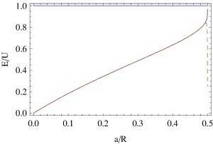
Figure 8: Plotted is the ratio of the exact interaction energy of two weakly-coupled spheres of equal radii to the proximity force approximation.

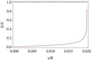
Figure 9: Plotted is the ratio of the exact interaction energy of two weakly-coupled spheres, with ratio of radii $b/a=49$, to the proximity force approximation.

In just the way indicated above, we can obtain a closed-form result for the interaction energy between a weakly-coupled sphere and a Dirichlet plane. Using the simplification that

$$\sum_{m=-l}^{l}(-1)^{m}\left(\begin{array}[]{ccc}l&l&l^{\prime}\\ m&-m&0\end{array}\right)\left(\begin{array}[]{ccc}l&l&l^{\prime}\\ 0&0&0\end{array}\right)=\delta_{l^{\prime}0},$$ (161)

we can write the interaction energy in the form

$$E=-\frac{\lambda a}{2\pi R}\int_{0}^{\infty}\rmd x\sum_{l=0}^{\infty}\sqrt{\frac{\pi}{2x}}(2l+1)K_{1/2}(x)I_{l+1/2}^{2}\left(x\frac{a}{R}\right).$$ (162)

Then in terms of $R/2$ as the distance between the center of the sphere and the plane, the exact interaction energy is

$$E=-\frac{\lambda}{2\pi}\left(\frac{a}{R}\right)^{2}\frac{1}{1-(2a/R)^{2}},$$ (163)

which as $a\to R/2$ reproduces the proximity force limit, contained in the (ambiguously defined) PFA formula

$$U=-\frac{\lambda}{8\pi}\frac{a}{d}.$$ (164)

The ratio of the exact interaction to the PFA is plotted in fig:exsppl.

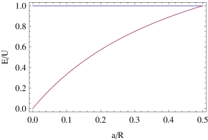
Figure 10: Plotted is the ratio of the exact interaction energy of a weakly-coupled sphere above a Dirichlet plane to the PFA.

4.3 Exact Results—Weak Coupling

In weak coupling it is possible to derive the exact (scalar) interaction between two potentials in general forms,

$$2D: \quad\mathfrak{E} =\frac{E}{L}=-\frac{1}{32\pi^{3}}\int(\rmd\mathbf{r_{\perp}})(\rmd\mathbf{r_{\perp}^{\prime}})\frac{V_{1}(\mathbf{r_{\perp}})V_{2}(\mathbf{r_{\perp}^{\prime}})}{|\mathbf{r-r^{\prime}}|^{2}},$$ (165)

$$3D: \quad E =-\frac{1}{64\pi^{3}}\int(\rmd\mathbf{r})(\rmd\mathbf{r^{\prime}})\frac{V_{1}(\mathbf{r})V_{2}(\mathbf{r^{\prime}})}{|\mathbf{r-r^{\prime}}|^{3}}.$$ (166)

The results found above in sections 4.1 and 4.2 can be directly derived from these pairwise summation formulæ. For exact results for $\delta$-function plates, see the contribution to this Proceedings by Jef Wagner.

It is straightforward to adapt the multiple scattering formalism to the far more relevant situation of electromagnetism. For weak coupling, this reduces to the (retarded dispersion) van der Waals (vdW) potential between polarizable molecule given by

$$V=-\frac{23}{4\pi}\frac{\alpha_{1}\alpha_{2}}{r^{7}},\qquad\alpha=\frac{\varepsilon-1}{4\pi N}.$$ (167)

This allows us to consider in the same vein (electromagnetic) interactions between distinct dilute dielectric bodies of arbitrary shape. (Of course, this potential represents the retarded limit of the van der Waals force. The non-retarded limit of the van der Waals force between bodies has long been studied, for example between dielectric cylinders [83, 84], and between a sphere and a plane [85].)

This vdW potential may be directly derived from the multiple scattering formula

$$W=-\frac{\rmi}{2}\mbox{Tr}\,\ln\frac{\boldsymbol{\Gamma}}{\boldsymbol{\Gamma}_{0}}\approx-\frac{\rmi}{2}\mbox{Tr}\,V_{1}\boldsymbol{\Gamma}_{0}V_{2}\boldsymbol{\Gamma}_{0},$$ (168)

where where have omitted self-action terms, and

$$\boldsymbol{\Gamma}_{0}=\boldsymbol{\nabla}\times\boldsymbol{\nabla}\times\mathbf{1}\frac{e^{-|\zeta||\mathbf{r-r^{\prime}}|}}{4\pi|\mathbf{r-r^{\prime}}|}+\mathbf{1}.$$ (169)

The quantity $V=\varepsilon-1$ is the potential representing the dielectric body.

We first apply this approach to compute the force between a dilute dielectric slab and an infinite dilute dielectric plate, as shown in pl-pl.

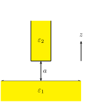
Figure 11: A plate of cross section $A$, a distance $a$ above an infinite plate. Both plates are of semi-infinite extent in the direction perpendicular to both plates.

If the cross sectional area of the finite slab is $A$, the force between the slabs is

$$\frac{F}{A}=-\frac{23}{640\pi^{2}}\frac{1}{a^{4}}(\varepsilon_{1}-1)(\varepsilon_{2}-1),$$ (170)

which is the Lifshitz formula for infinite (dilute) slabs. Note that there is no correction due to the finite area of the upper slab.

In the same way we can immediately compute the force between a dilute dielectric sphere of radius $a$ a distance $Z$ away from an infinite slab, as illustrated in sp-pl.

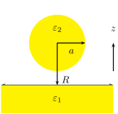
Figure 12: A dilute dielectric sphere, of radius $a$, the center of which is a distance $Z$ above an infinite dilute dielectric plate.

The interaction energy of this system is

$$E=-\frac{23}{640\pi^{2}}(\varepsilon_{1}-1)(\varepsilon_{2}-1)\frac{4\pi a^{3}/3}{Z^{4}}\frac{1}{(1-a^{2}/Z^{2})^{2}},$$ (171)

which agrees with the PFA in the short separation limit, $Z-a=\delta\ll a$, where the force is

$$F_{\rm PFA}=2\pi a\mathcal{E}_{\|}(\delta)=-\frac{23}{640\pi^{2}}(\varepsilon_{1}-1)(\varepsilon_{2}-1)\frac{2\pi a}{3\delta^{3}},$$ (172)

with an exact correction, intermediate between that for scalar averaged Dirichlet and Neumann [71, 72] and electromagnetic perfectly-conducting boundaries [73].

We can also consider torques between bodies. For example, consider a rectangular dilute dielectric solid, with sides $a$, $b$, and $c$, the center of mass of which is a distance $Z$ above a dilute dielectric plate, but which is tilted through an angle $\theta$ relative to the plate, as shown in tiltedslab.

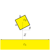
Figure 13: Rectangular solid (with dielectric constant $\varepsilon_{2}$) of side $a$, $b$, and $c$ (perpendicular to the plane, not shown) a distance $Z$ above an infinite plate (with dielectric constant $\varepsilon_{1}$) extending to $z=-\infty$. The side $b$ makes an angle $\theta$ with respect to the plate.

Generically, the shorter side wants to align with the plate, which is obvious geometrically, since that (for fixed center of mass position) minimizes the energy. However, if the slab has square cross section, the equilibrium position occurs when a corner is closest to the plate, also obvious geometrically. But if the two sides are close enough in length, a nontrivial equilibrium position between these extremes can occur, as well illustrated in eqtilt.

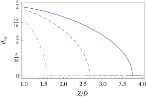
Figure 14: The stable equilibrium angle of a slab above an infinite plate for given $b/a$ ratios 0.95, 0.9, and 0.7, respectively given by solid, dashed, and dot-dashed lines.

For large enough separation, the shorter side wants to face the plate, but for

$$Z<Z_{0}=\frac{a}{2}\sqrt{\frac{2a^{2}+5b^{2}+\sqrt{9a^{4}+20a^{2}b^{2}+20b^{4}}}{5\left(a^{2}-b^{2}\right)}},\qquad a>b,$$ (173)

the equilibrium angle increases, until finally at $Z=D=\sqrt{a^{2}+b^{2}}/2$ the slab touches the plate at an angle $\theta=\arctan b/a$, that is, the center of mass is just above the point of contact, about which point there is no torque.

Finally, once again we can get exact results for the vdW interaction between parallel cylinders (radii $a,b$, center separation $R$):

$$\mathfrak{E}=\frac{E}{L}=-\frac{23}{60\pi}(\varepsilon_{1}-1)(\varepsilon_{2}-1)\frac{a^{2}b^{2}}{R^{6}}\frac{1-\frac{1}{2}\left(\frac{a^{2}+b^{2}}{R^{2}}\right)-\frac{1}{2}\left(\frac{a^{2}-b^{2}}{R^{2}}\right)^{2}}{\left[\left(1-\left(\frac{a+b}{R}\right)^{2}\right)\left(1-\left(\frac{a-b}{R}\right)^{2}\right)\right]^{5/2}},$$ (174)

and between spheres:

$$E=-\frac{23}{1920\pi}\frac{(\varepsilon_{1}-1)(\varepsilon_{2}-1)}{R}\Bigg{\{}\ln\left(\frac{1-\left(\frac{a-b}{R}\right)^{2}}{1-\left(\frac{a+b}{R}\right)^{2}}\right)$$

$$\mbox{}+\frac{4ab}{R^{2}}\frac{\frac{a^{6}-a^{4}b^{2}-a^{2}b^{4}+b^{6}}{R^{6}}-\frac{3a^{4}-14a^{2}b^{2}+3b^{4}}{R^{4}}+3\frac{a^{2}+b^{2}}{R^{2}}-1}{\left[\left(1-\left(\frac{a-b}{R}\right)^{2}\right)\left(1-\left(\frac{a+b}{R}\right)^{2}\right)\right]^{2}}\Bigg{\}}.$$ (175)

This last expression, which is rather ugly, may be verified to yield the proximity force theorem:

$$E\to U=-\frac{23}{640\pi}\frac{a(R-a)}{R\delta^{2}},\quad\delta=R-a-b\ll a,b.$$ (176)

It also, in the limit $b\to\infty$, $R\to\infty$ with $R-b=Z$ held fixed, reduces to the result esphpl for the interaction of a sphere with an infinite plate.

The same methodology may be used to derive the force between corrugated planes and corrugated concentric cylinders, which calculations may have relevance to nanomechanics. See the contribution to this Proceedings by Cavero-Peláez, and [80, 81].

5 Comments and Prognosis

In this talk I have described some recent exciting progress in the practical development of quantum vacuum energy. I have concentrated on the work of the Oklahoma group, without meaning to denigrate the work of many others of equal or greater importance. I will summarize the status of the topics I discussed briefly here:

• The temperature controversy can only be resolved by dedicated experiments, designed to measure Casimir forces at different temperatures between metal surfaces

• The semiconductor anomaly needs to be examined more closely both theoretically and experimentally.

• Casimir energies, including their divergent contributions, exhibit the inertial and gravitational masses expected: $m=E/c^{2}$. These gravitational interactions need to be examined for more complicated geometries, such as for the Casimir energy of a perfectly conducting spherical shell, with the hope of understanding the physical significance of the divergent contributions.

• The multiple-scattering methods recently developed are in fact not particularly novel, and illustrate the ability of physicists to continually rediscover old methods. What is new is the recognition that one can evaluate continuum determinants (or infinitely dimensional discrete ones) accurately numerically, and in some cases even exactly in closed form. This is making it possible to compute Casimir forces and torques for geometries previously inaccessible.

• It is indeed remarkable, if perhaps not surprising in retrospect, to see that closed form expressions can be obtained for the interaction between spheres, between parallel cylinders, and for other geometries in weak coupling. These results demonstrate most conclusively the unreliability of the proximity force approximation (of course, the proximity force theorem holds true).

• This methodology has been used to obtain new results for non-contact gears: See the talk by Inés Cavero-Peláez.

• Jef Wagner has presented new results for edge effects for semitransparent potentials.

• Undoubtedly these developments will lead to improved conceptual understanding, and to better comparison with experiment.

We thank the US National Science Foundation, grant number PHY-0554826, and the US Department of Energy, grant number DE-FG-04ER41305, for partial support of the research reported here. We especially thank Victor Dodonov for organizing such a successful meeting on “60 Years of the Casimir Effect,” and the International Center for Condensed Matter Physics at the University of Brasilia, and the College of Arts and Sciences and the office of the Vice President for Research at the University of Oklahoma for travel support. I thank my collaborators for allowing me to report on our joint work.

References

References

- [1] Casimir H B G 1948 Proc. Kon. Ned. Akad. Wetensch. 51 793
- [2] Brevik I, Ellingsen S A and Milton K A 2006 New J. Phys. 8 236 (Preprint quant-ph/0605005)
- [3] Klimchitskaya G L and Mostepanenko V M 2006 Comtemp. Phys. 47 131 (Preprint quant-ph/0609145)
- [4] Lifshitz E M 1955 Zh. Eksp. Teor. Fiz. 29 94
- [5] Boström M and Sernelius B E 2000 Phys. Rev. Lett. 84 4757
- [6] Høye J S, Brevik I, Aarseth J B and Milton K A 2003 Phys. Rev. E 67 056116 (Preprint quant-ph/0212125)
- [7] Jancovici B and Šamaj L 2004 J. Stat. Mech. P08006 (Preprint cond-mat/0407392)
- [8] Jancovici B and Šamaj L 2005 Europhys. Lett. 72 35 (Preprint cond-mat/0506363)
- [9] Buenzli P R and Martin Ph A 2005 Europhys. Lett. 72 42 (Preprint cond-mat/0506303)
- [10] Buenzli P R and Martin Ph A 2008 Phys. Rev. E 77 011114 (Preprint 0709.4194 [quant-ph])
- [11] Sernelius Bo E 2006 J. Phys. A: Math. Gen. 39 6741
- [12] Brevik I, Ellingsen S A, Høye J S and Milton K A 2008 J. Phys. A: Math. Theor. 41 164017 (Preprint 0710.4882 [quant-ph])
- [13] Høye J S, Brevik I, Ellingsen S A and Aarseth J B 2007 Phys. Rev. E 75 051127 (Preprint quant-ph/0703174)
- [14] Brevik I, Aarseth J B, Høye J S and Milton K A 2004 Proc. 6th Workshop on Quantum Field Theory under the Influence of External Conditions ed K A Milton (Paramus, NJ: Rinton Press) p 54 (Preprint quant-ph/0311094)
- [15] Obrecht J M, Wild R J, Antezza M, Pitaevskii L P, Stringari S and Cornell E A 2007 Phys. Rev. Lett. 98 063201 (Preprint physics/0608074)
- [16] Lamoreaux S K 1997 Phys. Rev. Lett. 87 5
- [17] Brevik I and Aarseth J B 2006 J. Phys. A: Math. Gen. 39 6187 (Preprint quant-ph/0511037)
- [18] Mohideen U and A. Roy A 1998 Phys. Rev. Lett. 81 4549 (Preprint physics/9805038)
- [19] Roy A, Lin C-Y, and Mohideen U 1999 Phys. Rev. D 60 111101(R) (Preprint quant-ph/9906062)
- [20] Harris B W, Chen F, and Mohideen U 2000 Phys. Rev. A 62 052109 (Preprint quant-ph/0005088)
- [21] Ederth T 2000 Phys. Rev. A 62 062104 (Preprint quant-ph/0008009)
- [22] Chan H B et al.2001 Phys. Rev. Lett. 87 211801 (Preprint quant-ph/0109046); Chan H B et al.2001 Science 291 1941
- [23] Chen F, Mohideen U, Klimchitskaya G L, and Mostepanenko V M 2002 Phys. Rev. Lett. 88 101801 (Preprint quant-ph/0201087)
- [24] Bressi G, Carugno G, Onofrio R, and Ruoso G 2002 Phys. Rev. Lett. 88 041804 (Preprint quant-ph/0203002)
- [25] Iannuzzi D, Lisanti M, and Capasso F 2004 Proc. Natl. Acad. Sci. USA 101 4019 (Preprint quant-ph/0403142)
- [26] Lisanti M, Iannuzzi D, and Capasso F 2005 Proc. Natl. Acad. Sci. USA 102 11989 (Preprint quant-ph/0502123)
- [27] Chen F, Klimchitskaya G L, Mostepanenko V M, and Mohideen U 2007 Phys. Rev. B 76 035338 (Preprint 0707.4390)
- [28] Decca R S et al.2005 Ann. Phys. NY 318 37 (Preprint quant-ph/0503105)
- [29] Bezerra V B et al.2006 Phys. Rev. E 73 028101 (Preprint quant-ph/0503134)
- [30] L. P. Pitaevskii 2008 Preprint 0801.0656v3
- [31] Geyer B, Klimchitskaya G L and Mostepanenko V M 2005 Phys. Rev. D 72 085009 (Preprint quant-ph/0510054)
- [32] Klimchitskaya G L, Geyer B, and Mostepanenko V M 2006 J. Phys. A: Math. Gen. 39 6495 (Preprint quant-ph/0602097)
- [33] Geyer B, Klimchitskaya G L, and Mostepanenko VM 2006 Int. J. Mod. Phys. A 21 5007 (Preprint 0704.1040)
- [34] Klimchitskaya G L and Geyer B 2008 J. Phys. A: Math. Gen. 41 164032 (Preprint 0802.3729)
- [35] Klimchitskaya G L, Mohideen U and Mostepanenko V M 2007 J. Phys. A: Math. Theor. 40 F841 (Preprint 0707.2734)
- [36] Castillo-Garza R, Chang C-C, Jimenez D, Klimchitskaya G L, Mostepanenko V M and Mohideen U 2007 Phys. Rev. A 75 062114 (Preprint 0705.1358 [quant-ph])
- [37] Chen F, Klimchitskaya G L, Mostepanenko V M and Mohideen U 2007 Optics Express 15 4823 (Preprint quant-ph/0610094)
- [38] Ellingsen S A, Brevik I, Høye J S and Milton K 2008 Phys. Rev. E 76 051127 (Preprint 0805.3065)
- [39] Ådnøy Ellingsen S A, Brevik I, Høye J S and Milton K 2008 Preprint 0809:0763
- [40] Brevik I and Milton K A 2008 Phys. Rev. E 78 011124 (Preprint 0802.2542 [quant-ph])
- [41] Fulling S A, Milton K A, Parashar P, Romeo A, Shajesh K V and Wagner J 2007 Phys. Rev. D 76 025004 (Preprint hep-th/0702091)
- [42] Milton K A, Parashar P, Shajesh K V and Wagner J 2007 J. Phys. A: Math. Theor. 40 10935 (Preprint 0705.2611 [hep-th])
- [43] Milton K A, Fulling S A, Parashar P, Romeo A, Shajesh K V and Wagner J A 2008 J. Phys. A: Math. Theor. 41 164052 (Preprint 0710.3841 [hep-th])
- [44] Boyer T H 1968 Phys. Rev. 174 1764
- [45] Graham N, Jaffe R L, Khemani V, Quandt M, Schroeder O and Weigel H 2004 Nucl. Phys. B 677 379 (Preprint hep-th/0309130), and references therein
- [46] Deutsch D and Candelas P 1979 Phys. Rev. D 20 3063
- [47] Cavero-Peláez I, Milton K A and Wagner J 2006 Phys. Rev. D 73 085004 (Preprint hep-th/0508001)
- [48] Cavero-Peláez I, Milton K A and Kirsten K 2007 J. Phys. A: Math. Theor. 40 3607 (Preprint hep-th/0607154)
- [49] Calloni E et al.2002 Phys. Lett. A 297 328 (Preprint hep-th/0302082)
- [50] Bimonte G et al.2006 Phys. Rev. D 74 085011 (Preprint hep-th/0606042)
- [51] Estrada R, Fulling S A, Liu Z, Kaplan L, Kirsten K and Milton K A 2008 J. Phys. A: Math. Theor. 41 164055
- [52] Brown L S and Maclay G J 1969 Phys. Rev. 184 1272
- [53] Milton K A 2001 The Casimir Effect: Physical Manifestations of Zero-Point Energy (Singapore: World Scientific), Sec. 11.1
- [54] Bimonte G, Esposito G and Rosa L 2008 Phys. Rev. D 78 024010 (Preprint 0804.2839 [hep-th])
- [55] Jaekel M T and Reynaud S 1993 Journal de Physique I 3 1093
- [56] Schwinger J 1970 Particles, Sources, and Fields (Reading, MA: Addison-Wesley)
- [57] Marzlin K P 1994 Phys. Rev. D 50 888
- [58] Milton K A 2004 J. Phys. A: Math. Gen. 37 R209 (Preprint hep-th/0406024)
- [59] Shajesh K V, Milton K A, Parashar P and Wagner J A 2008 J. Phys. A: Math. Theor. 41 164058 (Preprint 0711.1206 [hep-th])
- [60] Blocki J, Randrup J, Świa̧tecki W J and Tsang C F 1977 Ann. Phys. NY 105 427
- [61] Krein M G 1953 Mat. Sb. (N.S.) 33 597; 1962 Dokl. Akad. Nauk SSSR 144 268 [Sov. Math.-Dokl. 3 707]; Birman M Sh and Krein M G 1962 Dokl. Akad. Nauk SSSR 144 475 [Sov. Math.-Dokl. 3 740]
- [62] Renne M J 1971 Physica 56 125
- [63] Balian R and Duplantier B 1977 Ann. Phys. NY 104 300; Balian R and Duplantier B 1978 112 165; Balian R and Duplantier B 2004 Preprint quant-ph/0408124
- [64] Büscher R and Emig T 2005 Phys. Rev. Lett. 94 133901; Emig T, Jaffe R L, Kardar M, and Scardicchio A 2006 Phys. Rev. Lett. 96 080403 (Preprint cond-mat/0601055)
- [65] Reynaud S, Maia Neto P A, and Lambrecht A 2008 J. Phys. A: Math. Theor. 41 164004 (Preprint 0709.5452) (Preprint quant-ph/0410101); Maia Neto P A, Lambrecht A, and Reynaud S 2005 Europhys. Lett. 69 924; Maia Neto P A, Lambrecht A, and Reynaud S 2005 Phys. Rev. A 72 012115 (Preprint quant-ph/0505086); Lambrecht A, Maia Neto PA, and Reynaud S, 2006 New J. Phys. 8 243 (Preprint quant-ph/0611103)
- [66] Bulgac A, Marierski P, and Wirzba A 2006 Phys. Rev. D 73 025007 (Preprint hep-th/0511056); Wirzba A, Bulgac A and Magierski P 2006 J. Phys. A 39 6815 (Preprint quant-ph/0511057); Wirzba A 2008 J. Phys. A: Math. Theor. 41 164003 (Preprint 0711.2395)
- [67] Dalvit D A R, Lombardo F C, Mazzitelli F D, and Onofrio R 2006 Phys. Rev. A 74 020101(R) (Preprint quant-ph/0608033); Dalvit D A R, Lombardo F C, Mazzitelli F D, and Onofrio R 2006 New J. Phys. 8 240 (Preprint quant-ph/0610181)
- [68] Bordag M 2006 Phys. Rev. D 73 125018 (Preprint hep-th/0602295); Bordag M 2007 Phys. Rev. D 75 065003 (Preprint quant-ph/0611243)
- [69] Kenneth O and Klich I 2008 Phys. Rev. B 78 014103 (Preprint 0707.4017 [quant-ph])
- [70] Kenneth O and Klich I 2006 Phys. Rev. Lett. 97 160401 (Preprint quant-ph/0601011)
- [71] Wirzba A 2008 J. Phys. A: Math. Theor. 41 164003 (Preprint 0711.2395 [quant-ph])
- [72] Bordag M and Nikolaev V 2008 J. Phys. A: Math. Theor. 41 164002 (Preprint 0802.3633 [hep-th])
- [73] Maia Neto P A, Lambrecht A, and Reynaud S 2008 Phys. Rev. A 78 012115 (Preprint 0803.2444)
- [74] Emig T, Graham N, Jaffe R L and Kardar M 2007 Phys. Rev. Lett. 99 170403 (Preprint 0707.1862 [cond-mat.stat-mech])
- [75] Emig T, Graham N, Jaffe R L and Kardar M 2008 Phys. Rev. D 77 025005 (Preprint 0710.3084 [cond-mat.stat-mech])
- [76] Emig T and Jaffe R L 2008 J. Phys. A: Math. Theor. 41 164001 (Preprint 0710.5104 [quant-ph])
- [77] Milton K A and Wagner J 2008 J. Phys. A: Math. Theor. 41 155402 (Preprint 0712.3811 [hep-th])
- [78] Milton K A and Wagner J 2008 Phys. Rev. D 77 045005 (Preprint 0711.0774 [hep-th])
- [79] Milton K A, Parashar P and Wagner J 2008 Phys. Rev. Lett., in press (Preprint 0806.2880 [hep-th])
- [80] Cavero-Peláez I, Milton K A, Parashar P and Shajesh K V 2008 Phys. Rev. D 78 065018 (Preprint 0805.2776 [hep-th])
- [81] Cavero-Peláez I, Milton K A, Parashar P and Shajesh K V 2008 Phys. Rev. D 78 065019 (Preprint 0805.2777 [hep-th])
- [82] Lippmann B and Schwinger J 1950 Phys. Rev. 79 469
- [83] Mahanty J and Ninham B W 1976 Dispersion Forces (London: Academic Press)
- [84] Nyland G H and Brevik I 1994 Physica A 202 81
- [85] Noguez C, Román-Velázquez C E, Esquivel-Sirvent R and Villarreal C 2004 Europhys. Lett. 67 191 (Preprint quant-ph/0310068); Román-Velázquez C E, Noguez C, Villarreal C, Esquivel-Sirvent R 2004 Phys. Rev. A 69 042109 (Preprint quant-ph/0303172)