High redshift quasars in the COSMOS survey: the space density of $z>$ 3 X-ray selected QSOs

Abstract

We present a new measurement of the space density of high redshift ($z\simeq$ 3.0-4.5), X–ray selected QSOs obtained by exploiting the deep and uniform multiwavelength coverage of the COSMOS survey. We have assembled a statistically large (40 objects), X–ray selected ($F_{0.5-2keV}>$ 10^-15 erg cm^-2 s^-1), homogeneous sample of $z>$ 3 QSOs for which spectroscopic (22) or photometric (18) redshifts are available. We present the optical (color-color diagrams) and X–ray properties, the number counts and space densities of the $z>$ 3 X–ray selected quasars population and compare our findings with previous works and model predictions. We find that the optical properties of X–ray selected quasars are not significantly different from those of optically selected samples. There is evidence for substantial X–ray absorption (log$N_{H}>$ 23 cm^-2) in about 20% of the sources in the sample. The comoving space density of luminous ($L_{X}\hbox{\raise 2.15277pt\hbox{$>\lower 4.56386pt\hbox{$\kern-10.70009pt{\sim}$}$}}10^{44}$ erg s^-1) QSOs declines exponentially (by an e–folding per unit redshift) in the $z\sim$ 3.0–4.5 range, with a behavior similar to that observed for optically bright unobscured QSOs selected in large area optical surveys. Prospects for future, large and deep X–ray surveys are also discussed.

1 Introduction

The well known correlations between Super Massive Black Holes (SMBH) and galaxy properties such as bulge luminosity and stellar velocity dispersion (Gebhardt et al. 2000; Ferrarese & Merrit 2000), which are by now firmly established at least in the local Universe, point towards a tight link between the assembly of the bulge mass and SMBH. The high redshift AGN luminosity function (LF) and the source counts represent key observational constraints for theoretical models of galaxy and SMBH formation and evolution. While most models are reasonably successful in reproducing several observables in the high-luminosity regime (Di Matteo et al. 2005; Volonteri & Rees 2006; Hopkins et al. 2005; Lapi et al. 2006; Menci et al. 2008), they have to face the paucity of data, especially at high redshifts and low luminosities. Given that theoretical predictions are used to determine key physical parameters, such as the QSOs duty cycle, the BH seed mass function, and the accretion rates, a reliable observational estimate of the QSOs LF and evolution at high redshift is extremely important.

Large optical surveys, most notably the 2dF Quasar Redshift Survey (2QZ; Croom et al. 2004) and the Sloan Digital Sky Survey (SDSS; i.e. Richards et al. 2006) were able to accurately measure the shape of the LF up to $z\sim 2.0-2.5$ and to constrain the bright (M${}_{\rm B}<$ –25.5 or M${}_{\rm I}<$ –27.6, corresponding to bolometric luminosities of log$L_{bol}\hbox{\raise 2.15277pt\hbox{$>\lower 4.56386pt\hbox{$\kern-10.70009pt{\sim}$}$}}46$ erg s^-1) QSOs LF up to z $\sim$ 6.5: the space density of optically selected QSOs peaks at $z\sim 2-3$, then decreases approximately by a factor 3, per unit redshift, in the range $z\simeq 3-6$ (Schmidt, Schneider & Gunn 1995, Fan et al. 2001, 2004; Richards et al. 2006). The high–redshift quasar surveys mentioned above are relatively shallow and probe only the bright end of the LF. Recently, deep optical surveys were able to probe the LF at significantly fainter magnitudes using different selection criteria (e.g. Wolf et al. 2003, Hunt et al. 2004, Fontanot et al. 2007, Bongiorno et al. 2007, Siana et al. 2008). However, the statistics on the faint QSOs population at $z>3$ is still limited given the typically small area surveyed.

Moreover, optically selected quasars are known to make up only a fraction of the entire population of accreting SMBH: in fact, most of the accretion power in the Universe is obscured by large amounts of dust and gas (see, e.g., Fabian & Iwasawa 1999); moreover, AGN and QSOs span a broad range in accretion rate (see, e.g., Merloni & Heinz 2008), and, therefore, of intrinsic luminosities. Deep X-ray surveys with Chandra and XMM–Newton have proven to be very efficient in revealing obscured accretion (except for Compton Thick AGN) down to relatively low luminosities (see Brandt & Hasinger 2005 for a review). According to the most recent models for the synthesis of the X–ray Background (e.g. Gilli,Comastri & Hasinger 2007), the obscured AGN population (including heavily obscured Compton Thick AGN) outnumbers the unobscured ones by a luminosity dependent factor ranging from $\sim 2$ at L${}_{\rm X}\simeq 10^{45}$ erg s^-1 to $\sim 8$ at L${}_{\rm X}\simeq 10^{42}$ erg s^-1. The evidence for a decreasing obscured AGN fraction towards high luminosities is supported by many investigations (e.g. Ueda et al. 2003, Treister & Urry 2005). Moreover, there is also increasing evidence that the fraction of obscured AGN grows towards high redshifts (La Franca et al. 2005; Treister & Urry 2006; Hasinger 2008).

By combining deep and shallower X–ray surveys (Ueda et al. 2003; La Franca et al. 2005; Hasinger et al. 2005; Silverman et al. 2008) it has been possible to address the issue of the evolution of the X-ray LF at high redshifts. Previous works presented evidence for a decline of the comoving space density of X–ray selected AGN at $z>$ 3 in both the soft (0.5–2 keV; Hasinger et al. 2005; Silverman et al. 2005) and hard (2–10 keV; Silverman et al. 2008) bands with a rate similar to that observed for optically selected quasars. At face value, these findings would imply that the space density of obscured AGN, which are likely to be missed by optical surveys, declines toward high redshifts ($z>$ 3) with a behavior similar to that of the unobscured AGN, at least at the relatively high luminosities probed by present X–ray surveys (log$L_{X}\hbox{\raise 2.15277pt\hbox{$>\lower 4.56386pt\hbox{$\kern-10.70009pt{\sim}$}$}}44$). However, the results available so far are based on rather heterogeneous and relatively small samples, also affected by a significant level of spectroscopic incompleteness due to the faint magnitudes of the optical counterparts. To cope with this limitation, several photometric selection techniques have been proposed in the recent years. Though differing in the details, the search for high redshift, obscured AGN is mainly based on a suitable combination of X–ray, optical and infrared flux ratios (see e.g. Fontanot et al. 2007). More specifically, hard X–ray emission associated with extremely faint or even undetected optical counterparts and extremely red colors (from optical wavelengths up to mid–infrared) is considered a reliable proxy for a high redshift obscured AGN (see, e.g., Koekemoer et al. 2004; Brusa et al. 2005; Fiore et al. 2008). As an example, at the X-ray fluxes probed by the COSMOS survey, an X-ray to optical flux ratio f_X/f${}_{opt}>10$ efficiently selects high z, Compton thin obscured AGN (see Fiore et al. 2003). Most of them have red or extremely red (R-K$>5$) optical to near infrared colors and indeed f_X/f_opt and R-K are tightly correlated among X-ray selected sources (Brusa et al. 2005). Unfortunately, due to the widely different selection criteria, it is difficult to combine the above mentioned approaches to obtain a reliable estimate of their space density. Given the importance of the AGN LF at high redshift for our understanding of SMBH growth and evolution, the search for and the census of high redshift ($z>$ 3) AGN warrant further efforts. The excellent multiwavelength coverage of the COSMOS field (Scoville et al. 2007) offers the unique opportunity to assemble the first statistically large, homogeneous, and well defined sample of X–ray selected, high redshift AGN, which is almost completely unbiased against obscuration up to column densities of the order of $N_{H}\simeq 10^{23}$ cm^-2.

The paper is structured as follows. In Section 2 we describe the sample selection which is mainly based on the optical and multiwavelength identification of the XMM–COSMOS survey (Hasinger et al. 2007, Cappelluti et al. 2007, 2008, Brusa et al. 2007; 2008), complemented by Chandra positions when available (Elvis et al. 2008, Puccetti et al. 2008, Civano et al. 2008) to secure the correct optical counterpart, and, most importantly, by spectroscopic (Trump et al. 2008, Lilly et al. 2007) and high-quality photometric redshifts (Salvato et al. 2008). The optical and X–ray properties are presented in Section 3 and 4, respectively. In Section 5 the number counts and space density of the sample are discussed and compared with model predictions. The results are summarized in Section 6, where the perspectives for future observations are also briefly outlined. A $H_{0}=70$ km s^-1 Mpc^-1, $\Omega_{M}$ = 0.3 and $\Omega_{\Lambda}$ = 0.7 cosmology is adopted. Optical magnitudes are in the AB system.

2 The sample

2.1 Parent sample

The Cosmic Evolution Survey (COSMOS) field (Scoville et al. 2007) is a so far unique area for deep and wide comprehensive multiwavelength coverage, from the optical band with Hubble, Subaru and other ground based telescopes, and infrared with Spitzer, and X-rays with XMM–Newton and Chandra, to the radio with the VLA. The spectroscopic coverage with VIMOS/VLT and IMACS/Magellan, coupled with the reliable photometric redshifts derived from multiband fitting, is designed to be directly comparable, at $0.5<z<1.0$, to the 2dFGRS (Colless et al. 2001) at $z\sim 0.1$, and to probe the correlated evolution of galaxies, star formation, AGN, and dark matter with large-scale structure in the redshift range $z\sim$ 0.5–4.

The COSMOS field has been observed with XMM-Newton for a total of $\sim 1.5$ Ms at a rather homogeneous depth of $\sim 50$ ks (Hasinger et al. 2007, Cappelluti et al. 2007, 2008). The catalogue used in this work includes 1848 point–like sources above a given threshold with a maximum likelihood detection algorithm in at least one of the soft (0.5–2 keV), hard (2–10 keV) or ultra-hard (5–10 keV) bands down to limiting fluxes of $\sim$ 5$\times 10^{-16}$, $\sim$ 3$\times 10^{-15}$ and $\sim$ 5$\times 10^{-15}$ erg cm^-2 s^-1, respectively (see Cappelluti et al. 2007, 2008 for more details). The adopted likelihood threshold corresponds to a probability $\sim 4.5\times 10^{-5}$ that a catalog source is a spurious background fluctuation. Following Brusa et al. (2008), we further excluded from this catalog 24 sources which turned out to be a blend of two Chandra sources and additional 26 faint XMM sources coincident with diffuse emission (Finoguenov et al. 2008). To maximize the completeness over a well defined large area and, at the same time, keep selection effects under control, we considered only sources detected above the limiting flux corresponding to a coverage of more than 1 deg² in at least one of the three X–ray energy ranges considered, namely: 1$\times 10^{-15}$ erg cm^-2 s^-1, 6$\times 10^{-15}$ erg cm^-2 s^-1, and 1$\times 10^{-14}$ erg cm^-2 s^-1, in the 0.5–2 keV, 2–10 keV or 5–10 keV bands, respectively (Cappelluti et al. 2008). The final sample includes therefore 1651 X–ray sources. The combination of area and depth is similar to the one of the sample studied by Silverman et al. (2008, see their Fig. 8). The main difference is given by the considerably higher redshift completeness of the parent sample obtained thanks to the much deeper coverage in the optical and near IR bands and the systematic use of photometric redshifts (see below) to avoid the need for substantial corrections for completeness (see discussion in Silverman et al. 2008).

A detailed X–ray to optical association has been performed (Brusa et al. 2008), applying the likelihood ratio technique on the optical, near-infrared (K–band) and mid–infrared (IRAC) catalogs available. In addition, for the subsample of the XMM-COSMOS sample covered by Chandra observations ($\sim$ 50% of the total sample), the ACIS images have been visually inspected to further exclude possible misidentifications problems. Of the 1651 sources in the XMM–COSMOS catalog described above, 1465 sources have a unique/secure optical counterpart from the multiwavelength analysis, i.e. among them we expect only $\sim$ 1% of possible misidentifications (see discussion in Brusa et al. 2008). For additional 175 sources, the proposed optical counterpart has about 50% probability to be the correct one. Given that the alternative counterparts of these 175 sources show optical to IR properties and redshift distribution comparable to the primary ones, the proposed ones can be considered statistically representative of the true counterparts of the X-ray sources. Therefore we consider also those in our analysis. Finally, 11 sources remain unidentified, because it was not possible to assign them to any optical and/or infrared counterpart.

Spectroscopic redshifts for the proposed counterparts are available from the Magellan/IMACS and MMT observation campaigns ($\sim 590$ objects, Trump et al. 2007, Trump et al. 2008), from the zCOSMOS project ($\sim 350$ objects, Lilly et al. 2007), or were already present either in the SDSS survey catalog ($\sim 100$ objects, Adelman-McCarthy et al. 2005, Kauffman et al. 2003), or in the literature ($\sim 95$ objects, Prescott et al. 2006). In summary a total of 683 independent, good quality spectroscopic redshifts are available corresponding to a substantial fraction ($\sim 40$%) of the entire sample.

Photometric redshifts for all the XMM–COSMOS sources have been obtained exploiting the COSMOS multiwavelength database and are presented in Salvato et al. (2008). Since the large majority of the XMM–COSMOS sources are AGN, in addition to the standard photometric redshift treatments for normal galaxies, a new set of SED templates has been adopted, together with a correction for long–term variability and luminosity priors for point-like sources (see Salvato et al. 2008 for further details). Moreover, the availability of the intermediate band Subaru filters (Taniguchi et al. 2008) is crucial in picking up emission lines (see also Wolf et al. 2004). This led, for the first time for an AGN sample, to a photometric redshift accuracy comparable to that achieved for inactive galaxies ($\sigma_{\Delta z/(1+z)}\sim 0.015$ and $\sim 5$% outliers) at i$<\lower 4.56386pt\hbox{$\kern-10.70009pt{\sim}$}$22.5. At fainter magnitudes (22.5 $<I<24.5$) the dispersions increases to $\sigma_{\Delta z/(1+z)}\simeq 0.035$ with $\sim$ 15% outliers, still remarkably good for an AGN sample.

A photometric redshift is available for all but 36 objects out of 1651 in the flux limited sample. Fourteen of them do not have multiband photometry, being detected only in the IRAC and K bands. The remaining 22 objects are affected by severe blending problems making the photo-z estimate not reliable.

Figure 1: Spectra of the 22 spectroscopically confirmed z$>3$ quasars, in order of increasing redshift. The spectra are shown in the observed frame and the main emission and absorption features are labelled. The four objects with single line spectra are marked with a “:” right to the redshift. The source of the spectra (IMACS, zCOSMOS or MMT is reported in the top right of each panel).

Fig. 1. — Continued.

Fig. 1. — Continued.

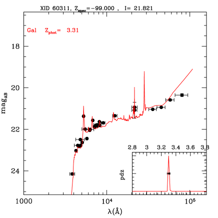
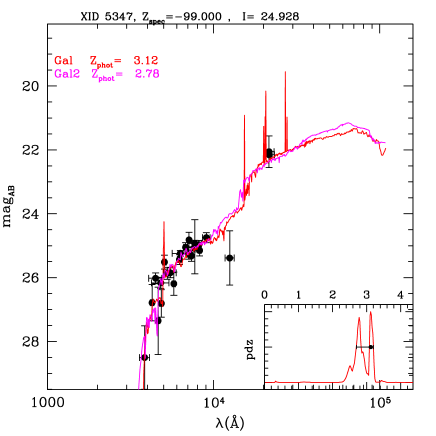
Figure 2: Two examples of photometric redshift determination for sources without a spectroscopic redshift: a photoz with a unique solution (XID 60311) and an object with two possible solutions for the photometric redshift (XID 5347). Black points are the observed photometry from the U-band to IRAC 8.0$\mu$m. The red curve is the best fit template. The inset in the bottom right shows the probability distribution function (normalized to one) as a function of redshift.

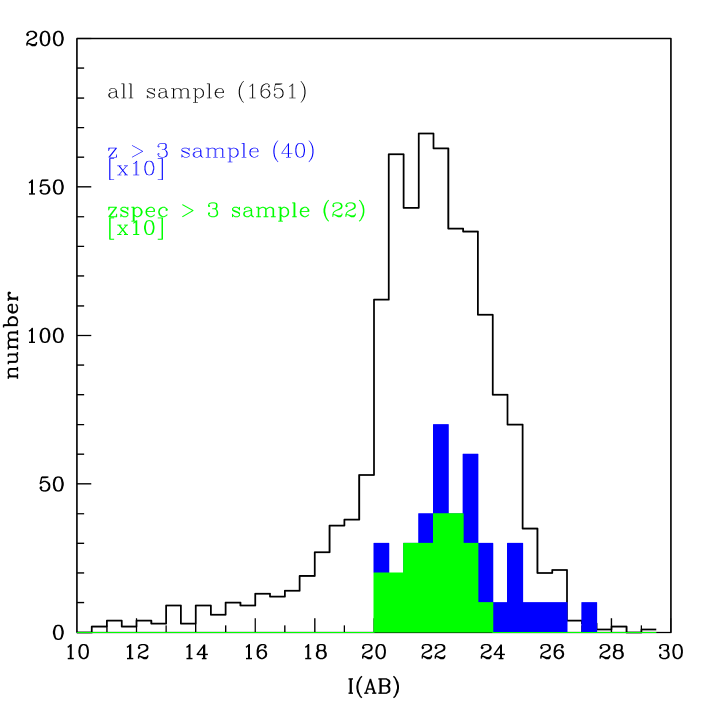
Figure 3: Histogram of the i-band magnitude distribution for the global XMM–COSMOS sample (empty), the $z>3$ sample (blue) and the spectroscopic $z>$ 3 sample (green)

2.2 The z$>3$ QSOs sample

We used the combined spectroscopic and photometric information available on the redshifts in our XMM–COSMOS sample to select the sample of $z>3$ quasars. There are 40 XMM–COSMOS sources which have a spectroscopic (22) or, when spectroscopic redshifts are not available, photometric (18) redshifts larger than $z>3$. Nineteen of them are detected in both the soft and hard bands, 20 are detected only in the soft band at fluxes larger than 1$\times 10^{-15}$ erg cm^-2 s^-1 and 1 object is detected only in the hard band above the chosen threshold of 6$\times 10^{-15}$ erg cm^-2 s^-1, while it is just below the adopted limiting flux in the soft band.

Table 1 lists the name of the objects (following the standard IAU notation), the X–ray identifier number from the XMM-COSMOS catalog (Cappelluti et al. 2008) used as reference identifier in the following, the identifier number from the COSMOS photometric catalog (Capak et al. 2007) and the coordinates of the optical counterparts.

The basic properties (photometric and spectroscopic redshifts, I–band magnitude, X–ray fluxes and luminosities, and hardness ratio) for these objects are reported in Table 2. The optical photometry used to derive the photometric redshifts can be retrieved by the public COSMOS photometric catalog available at IRSA via the optical identifier number provided in the 3rd column of Table 1. The deep Chandra survey in the COSMOS field covers about 0.9 deg² in the central region. Chandra images are available for about half (19) of the high–z QSOs in our sample and for these objects the identification of the counterparts is secure, thanks to the positional accuracy provided by Chandra spatial resolution. Following the discussion in Brusa et al. (2008), we expect that, among the 21 sources without Chandra coverage, at most one can be a misidentification.

Spectroscopic redshifts are available for 22 sources, and are reported in Table 2. The observed frame spectra, sorted in order of ascending redshift, are shown in Figure 1, with all the major emission lines labeled. For 4 of them, the spectroscopic redshift is based on a single, broad line identified as CIV1549 or Ly$\alpha$. In all four cases, the photometric redshift rules out alternative solutions at lower-redshift, favoring the proposed $z>3$ nature.

In all but two cases there is convincing evidence for the presence of broad optical lines. For two sources (XID 5162 and XID 5606) the most prominent emission lines are narrow (FWHM$<1500$ km s^-1) and thus these objects are candidate Type 2 QSOs.

For the remaining 18 sources, only photometric redshifts are available. The photometric redshifts for the entire $z>3$ sample, with associated errors (1$\sigma$) are reported in Table 2. A detailed discussion on the quality and reliability of AGN photometric redshifts is presented elsewhere (Salvato et al. 2008). Here we limit to note that all but one (XID 2407) of the objects with spectroscopic redshifts have photometric redshifts well consistent with the spectroscopic ones, with  60% of the spectroscopic redshifts being within the 1$\sigma$ range of the photometric redshifts. Moreover, also the fraction of outliers (1 source out of 22) is consistent with the expectations for the entire photo-z catalog (5%, see Section 2.1). However, we should also note that spectroscopic redshifts are available for the brightest (i$\hbox{\raise 2.15277pt\hbox{$<\lower 4.56386pt\hbox{$\kern-10.70009pt{\sim}$}$}}23$) sample and a higher fraction of outliers (up to  15%) is expected at fainter optical magnitudes.

Salvato et al. (2008) also computed probability distribution functions (PDF) for the photometric redshift solution. In the sample of 40 quasars, five objects have the first solution (i.e. the highest value of PDF) at $z>3$, but a comparable solution (in terms of PDF) at $z<3$ exists. Most of these objects have i$\hbox{\raise 2.15277pt\hbox{$>\lower 4.56386pt\hbox{$\kern-10.70009pt{\sim}$}$}}24$. Conversely, there are additional 14 objects in the entire sample of XMM–COSMOS counterparts which present the first solution at $z<3$, but have a second solution at $z>3$. Figure 2 shows two examples of the SED fitting and photometric redshift determination for a source with a reliable solution (XID 60311, left panel) and for an object with multiple, secondary solutions at lower redshift (XID 5347, right panel). Weighting the objects with the relative PDF, we obtain that $\sim 60$% of the sample of the 32 objects without spectroscopic redshifts and with either unique, first or second solution at $z>3$ are expected to be at $z>3$. This translates in $\sim 20$ objects, close to the 18 objects with primary solution at $z>3$, which are listed in Table 2.

Among the 22 sources lacking a photometric redshift, due to problems related to blends or saturation, six have spectroscopic redshifts which place them at $z<1.5$. We expect that the redshift distribution of these sources follows the one of the total sample, with only 3% (22/683, e.g. $\sim 1$ object) being at $z>3$. It should also be noted that the 14 objects undetected in the optical bands (10 of them detected in the soft band above the adopted limiting flux) and without an estimate of the photometric redshift, are candidate high redshift, possible obscured QSOs (see, e.g. Koekemoer et al. 2004, Mignoli et al. 2004).

Summarizing, we conclude that, although the fraction of objects in our sample which have only a photometric redshift is close to 50%, the total number of objects with $z>3$ is statistically robust. Even if some of the 18 objects without spectroscopic redshift are likely to be at $z<3$, this number is expected to be almost exactly compensated by the number of objects which, being at $z>3$, have instead their best photometric solution at $z<3$. Therefore, we consider the 40 objects listed in Table 2 as representative of the real number of sources at $z>3$. We will quantify in Section 6 the possible contribution of objects undetected in the optical bands to the total number of $z>3$ QSOs.

Figure 3 shows the magnitude distribution of the $z>3$ sample (blue filled histogram) compared with the overall optical population (black open histogram). The median magnitude of the $z>3$ sample (i=22.72, with a dispersion of 1.02 mag) is about 0.8 magnitudes fainter than that of the overall XMM–COSMOS population ($i=21.90$, with a dispersion of 1.32). Spectroscopically confirmed $z>$ 3 objects (green histogram in the figure) are in the bright tail of the magnitude distribution of the high redshift sample. A non negligible fraction of the objects in the sample (7/40) has $i>$ 24.5 and, as pointed out above, a somewhat more uncertain photo-z solution (see Table 2).

3 Optical colors

Multiband optical photometry provides a routinely-adopted, reliable selection technique to select high redshift QSOs. The method was first applied to AGN in the 1960s, based on the inference that quasars often have a larger ultraviolet excess than the hottest stars (Sandage & Wyndham 1965), and subsequently extended to large-scale surveys (e.g. Schmidt & Green 1983, Croom et al. 2001, Fan et al. 2001, Richards et al. 2006). The most suitable combination of colors strongly depends on the redshift range. For example, the ”UV excess” technique is optimal for $z<$ 2.0–2.2. At $z>$ 3 an efficient selection method is known as Lyman Break technique and has been extensively used to select $z>$ 3 QSOs and galaxies (see, e.g., Steidel et al. 1996, Hunt et al. 2004, Aird et al. 2008). Assuming a standard QSO template and including absorption by the Intergalactic Medium (IGM, i.e. the Lyman-alpha forest), it is possible to efficiently isolate $z>$ 3 QSOs in the $U-g^{\prime}$ vs $g^{\prime}-r^{\prime}$ color-color plane (i.e. Siana et al. 2008).

A somewhat different color–color plot ($v-i$ vs. $B-v$) has been extensively discussed by Casey et al. (2008): for efficient selection at $z>3$ they make a diagonal cut in the two color diagram, described by the relation: $v-i<1.15\times(B-v)-0.31$. The three photometric bands have been chosen in order to minimize the problems due to AGN variability: COSMOS observations in the $B,v$ and $i$ bands were taken at the same epoch, providing almost simultaneous colors, while the $g^{\prime}$ and $U$ band observations were taken about one year apart (Taniguchi et al. 2007, Capak et al. 2007).

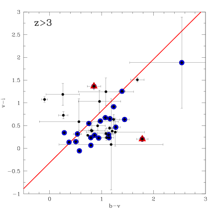
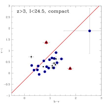
Figure 4: Left panel: $v-i$ vs. $B-v$ color–color diagram for the $z>3$ sources. Black points correspond to all $z>3$ sources, blue circles to the 20 objects classified as BL AGN, red triangles refer to the 2 objects classified as NL AGN. Outliers from the QSOs locus are those on the left of the red solid line, defined as: [$v-i<1.15\times(B-v)-0.31$]. Right panel: same as the previous panel, but only for the subsample with $i<24.5$ and compact morphology.

The X–ray selected QSOs of our sample are plotted in the $v-i$ vs. $B-v$ plane in Figure 4 (left panel) with associated errors. The 20 spectroscopically confirmed BL AGN are marked with blue circles, while the 2 objects classified as NL AGN are shown as red triangles. Eight objects ($\sim 20$%) lie above the nominal line proposed by Casey et al. (2008) to select $z>3$ QSOs in the COSMOS field. Among them two sources (XID 2407 and XID 5606) have a spectroscopic redshift. These objects would have not been selected as high redshift quasars from this optical color–color diagram. We should note, however, that the Casey et al. (2008) criterion was tested for relatively bright ($i<$ 24.5) sources with compact morphology defined in terms of Gini coefficient larger than $\sim 0.8$. If we further impose the same optical limit to the objects of our sample, and consider only the objects classified as point-like from the ACS analysis (Leauthaud et al. 2007), only 3 out of 25 ($\sim$ 12%) lie above the dividing line (Fig. 4, right panel). The eight objects above the dividing line in the left panel of Fig. 4 are, therefore, on average, optically faint ($i>$ 24.5) and/or with an extended morphology. These objects would not have been selected as high redshift candidates by an optical survey. We name these objects “outliers” and investigate their average X–ray properties in the following. Conversely, if we consider the full sample of XMM sources with $i<24.5$ and “compact” morphology, there is a total of 60 objects that lie below the diagonal line in Fig. 4: 25 shown in the right panel of Fig. 4 plus 35 additional objects. The majority of these 35 objects (25/35) has a good quality spectroscopic redshift lower than 3, and in most of the cases (20/25) they are classified as BL AGN at $z\sim$ 1–3. As discussed by Casey et al. (2008) the contamination of low–redshift sources in this optical color–color diagram can be as high as 50–70%.

4 X–ray properties

For each object with given redshift (either spectroscopic or photometric) the flux in the rest frame 2–10 keV band has been calculated, assuming the spectral slope derived from the ratio of the fluxes in the rest-frame hard and soft band. Rest frame 2–10 keV fluxes have been then converted into luminosities within the adopted cosmology. Figure 5 (left panel) shows the histogram of the rest frame, 2–10 keV luminosities for the 40 sources in the present sample. The rest frame 2–10 keV luminosities calculated using the observed 0.5–2 keV fluxes (roughly corresponding to the rest frame 2–10 keV fluxes at z$\geq 3$) are consistent with those derived with the method described above (see black histogram in Figure 5). All the objects in the $z>3$ sample have hard X–ray (2–10 keV) rest–frame luminosities in the interval 10⁴⁴-10⁴⁵ erg s^-1. The luminosity-redshift plane in the redshift interval $z$=3.0–4.5 is shown in Figure 5 (right panel). Sources with a spectroscopic redshift are plotted with blue (20 BL AGN) and red (2 NL AGN) symbols. The continuous line represents the luminosity limit of the survey computed from the 0.5–2 keV limiting flux.

The Hardness Ratio HR (defined as (H–S)/(H+S), where H and S are the counts detected in the 2–10 keV and 0.5–2 keV bands, respectively) as a function of the redshift for all the 40 objects in our sample is shown in Figure 6. For the 20 sources detected only in the soft band, upper limits have been obtained by conservatively assuming 25 hard counts. Loci of constant $N_{H}$ at different redshifts for a power law spectrum with $\Gamma=1.7$ are also reported with dashed lines. The shaded region marks the expected HR for an unabsorbed power-law with $\Gamma=1.7$ (upper limit) and $\Gamma=1.8$ (lower limit). The objects in our sample span a rather large range of HR and corresponding $N_{H}$ values, from unobscured to column densities up to logN${}_{H}\simeq 23.7$.

To increase the statistics and gain information on the average spectral properties of the different sources in the sample, we performed a stacking analysis of the source spectra. The spectra were extracted for all the sources in their rest-frame 2–22 keV band from the EPIC pn data and corrected for the local background, following the procedure outlined in Mainieri et al. (2007). Three sources (XID 5259, 5592, and 5594), which have null or negative counts in this energy range when the local background is subtracted, are excluded from the analysis here. Two additional sources (60186 and 60311) which do not show stringent upper limits in the HR are further excluded. The individual spectra were then corrected for the instrumental response curve, brought to the rest-frame and stacked together with energy intervals of 1 keV. Noisy spectral channels of the stacked spectra were binned further, when appropriate.

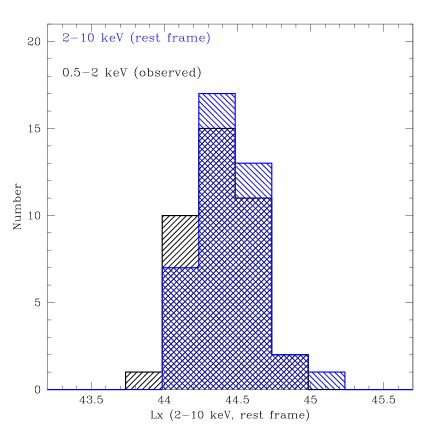
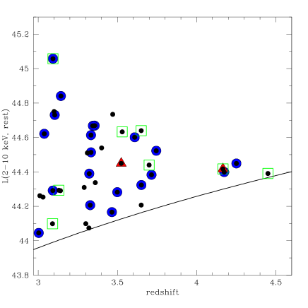
Figure 5: Left panel: Histogram of the rest frame 2–10 keV luminosity calculated assuming the spectral slope derived from the ratio of the fluxes in the rest frame soft and hard bands (blue histogram, see text for details) compared with the rest frame 2–10 keV luminosities calculated using the observed 0.5-2 keV fluxes (i.e., the rest frame 2-10 keV flux at z$>3$, black histogram). Right panel: the luminosity redshift plane for the objects in our sample. Symbols as in previous figures. Green squares mark the outliers from the optical color-color diagram of Fig. 4. The continuous line represents the luminosity limit of the survey computed from the 0.5–2 keV limiting flux.

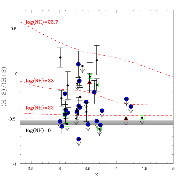
Figure 6: HR vs. redshift for the $z>3$ QSOs sample (symbols as in previous figures). The dashed lines correspond to the loci of constant $N_{\rm H}$ for a power-law spectrum with $\Gamma=1.7$. The shaded region marks the expected HR for an unabsorbed power law with $\Gamma=1.8$ (lower limit) and $\Gamma=1.7$ (upper limit).

At first, we divided the sample into two sub-samples based on the HR: the sources showing an indication of “soft” spectrum from the HR (i.e., the 26 objects below the locus of $N_{\rm H}=10^{23}$ cm^-2 at different redshifts) and the sources with an indication of a “hard” spectrum (i.e., the 9 objects above the $N_{\rm H}=10^{23}$ cm^-2 locus). The stacked spectra for these two sub–samples are shown in Figure 7 and the results from a power-law fit are summarized in Table 3. The “soft” sources (open squares in Fig. 7) have a steeper spectral slope ($\Gamma\sim 1.8\pm 0.3$) than the “hard” sources (filled squares: $\Gamma\sim 0.9\pm 0.8$), demonstrating that the HR analysis (which is based on the X–ray color in the observed frame) can isolate the most absorbed sources even at these high redshifts.

The fraction of log $N_{\rm H}\geq 23$ AGN, computed weighting with the errors the number of sources with HR above the log$N_{\rm H}$=23, is $\sim 20$%, somewhat larger than the Gilli et al. (2007) expectations ($\sim 10$%) for the same luminosity, redshifts and flux limits of our survey.

It is interesting to note that one of the two objects with narrow emission lines in the optical spectrum (XID 5162, z=3.524) has an HR ($\sim-0.11$, red triangle in Fig. 6) consistent with a column density log$N_{H}>23$ and therefore would be classified as a Type 2 QSO from both the optical and the X-ray diagnostics. This object is one of the highest redshift, radio quiet, spectroscopically confirmed Type 2 QSO (see e.g. Norman et al. 2002, Mainieri et al. 2005). The other two objects with log$N_{H}>$ 23 and spectroscopic redshift (XID 60131 at z=3.328, and XID 1151 at z=3.345) show clear signatures of broad absorption lines (BAL) in their optical spectra (Fig. 1). Column densities of the order of log$N_{H}\sim$ 23 are common among those BAL QSOs for which good quality X–ray spectra are available (Gallagher et al. 2002). Significant X–ray absorption in BAL QSOs is detected up to $z\sim$ 3 (Shemmer et al. 2005).

It is important to note, however, that the HR at $z>3$ is not very sensitive to column densities below log$N_{\rm H}\simeq$23. Given also the typical dispersion in the intrinsic power-law spectra, it is possible that the sub-sample of “soft” sources contains also some of these absorbed AGN. These sources are expected to be optically faint (e.g. Alexander et al. 2001, Fiore et al. 2003, Mainieri et al. 2005, Cocchia et al. 2007) and thus among the still spectroscopically unidentified sources. In order to test this possibility, we further divided the “soft” sample into two subsamples: sources without a spectroscopic redshift available (10) and sources spectroscopically identified as BL AGN (16, see Figure 7, right panel). There is evidence of absorption (below $\sim$ 3 keV, corresponding to log$N_{\rm H}\sim$22.5) in the average spectrum of spectroscopically unidentified sources. The X–ray counting statistics does not allow to establish, on a source by source basis, whether the ”outliers” of optical color–color diagrams are also obscured in the X–rays. Given that the five ”outliers” from the optical color–color diagram make up about 30% of this absorbed sample, it may well be possible that they are responsible of the low energy cut–off in the stacked spectrum (right panel of Fig. 7).

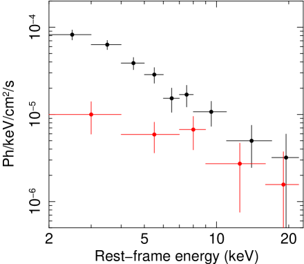
Figure 7: Left panel: Rest-frame stacked spectra of sources with logNH$<23$ at all redshifts (26 objects, black circles) and with logNH$>23$ (9 objects, red circles). Right panel: Rest-frame stacked spectra of the sources with with logNH$<23$ further divided in BL AGN (16 objects, squares) and spectroscopically unidentified sources (10 objects, triangles).

5 Evolution of $z>3$ QSOs

5.1 Number counts

We derived the logN–logS of the $z>3$ XMM–COSMOS QSOs by folding the observed flux distribution with the sky coverage. The binned logN–logS relation of the 39 objects with a 0.5–2 keV flux larger than 10^-15 erg cm^-2 s^-1 is plotted in Figure 8 (red points, with associated Poissonian errors). The green shaded area represents an estimate of the maximum and minimum number counts relation at $z>$ 3 under somewhat extreme assumptions. The lower bound is obtained by considering only the 22 sources with a spectroscopic redshift, while the upper bound includes in the $z>$ 3 sample also the 10 objects with a 0.5–2 keV flux larger than 10^-15 erg cm^-2 s^-1and without a detection in the optical band and the 11 objects above the same flux threshold and with a second photometric redshift solution at $z>3$ (see $\S$2). Under these assumptions, the lower limit corresponds to the (very unlikely) hypothesis that all the photometric redshifts are overestimated, while the upper limit corresponds to the assumption that the non–detection in the optical band is a very reliable proxy of high redshift in X-ray selected samples (e.g. Koekemoer et al. 2004; Koekemoer et al. 2008). The dashed blue curve corresponds to the predictions of the XRB synthesis model (Gilli et al. 2007), obtained extrapolating to high-z the best fit parameters of Hasinger et al. (2005), while the solid blue curve represents the model predictions obtained introducing in the LF an exponential decay with the same functional form ($\Phi(z)=\Phi(z_{0})\times 10^{-0.43(z-z_{0})}$) adopted by Schmidt et al. (1995) to fit the optical LF, corresponding to an e–folding per unit redshift.

The model predictions at $z>$ 3 obtained extrapolating the Hasinger et al. (2005) best fit parameters at high-z (dashed line) clearly overestimate the observed counts even in the most optimistic scenario (upper boundary in Fig. 8). A much better description to the observed counts is obtained by introducing the exponential decline in the X–ray LF at $z>$ 2.7 (i.e. we have here adopted $z_{0}=2.7$ following Schmidt et al. 1995).

An estimate of the number counts for $z>$4 QSOs is also reported in Fig. 8. Although only 4 objects are detected in the XMM–COSMOS survey, there is a remarkably good agreement with the predicted number counts, suggesting that the Schmidt et al. (1995) parameterization provides a good description of the X–ray selected QSOs surface densities up to $z\simeq$ 4.5.

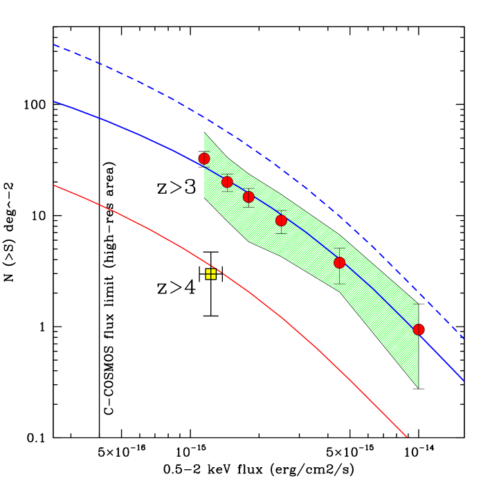
Figure 8: The binned LogN-logS relation (red circles with associated Poissonian errors) of the z$>3$ QSOs population. The dashed and solid blue curves correspond to two different predictions based on the Gilli et al. (2007) model. The former is obtained extrapolating the best fit parameters of Hasinger et al. (2005) for the evolution of the X–ray LF to high-z, while an exponential decay at $z>$ 2.7 is introduced in the latter. The green shaded area represents an estimate of the global error budget (see text for details). The yellow square (with associated Poissonian error) is the estimate of the number counts for $z>$ 4 quasars based on the 4 objects (3 of them with a spectroscopic redshift) in the XMM–COSMOS sample. The red curve shows the predicted number counts assuming the exponential decay in the LF. The vertical line at $4\times 10^{-16}$ erg cm^-2 s^-1 represents the limit of the C-COSMOS survey.

5.2 Comoving space densities

The comoving space density of $z>$ 3 QSOs in three, almost equally populated, redshift bins ($z=3.0-4.5$) is reported in Figure 9. The comoving space densities have been computed with the 1$/V_{max}$ method, originally proposed by Schmidt (1968), which takes into account the fact that more luminous objects are detectable over a larger volume. In order to reduce the effects of incompleteness (see Fig. 5 right panel), the space densities have been computed for luminosities logL${}_{X}>44.2$ (i.e. considering only 34 out of 39 objects). Because of the significant effects introduced by X-ray absorption, some particular care is needed in computing V_max for X-ray selected sources. In fact, for any given intrinsic luminosity, the effective limiting flux for detecting obscured sources is higher than for unobscured ones and the corresponding volume over which obscured sources can be detected is smaller. We therefore calculate the maximum available volume for each source using the formula:

$$V_{max}=\int_{z_{min}}^{z_{max}}\Omega(f(L_{x},z,N_{H}))\frac{dV}{dz}dz$$

where $\Omega(f(L_{x},z))$ is the sky coverage at the flux $f(L_{x},z)$ corresponding to a source with absorption column density $N_{H}$ and unabsorbed luminosity $L_{X}$, and $z_{max}$ is the maximum redshift at which the source can be observed at the flux limit of the survey. More specifically, for unabsorbed sources we adopted the observed rest–frame 2–10 keV luminosity (see $\S$4), while for obscured ones the unabsorbed luminosity was derived assuming the best fit column density as obtained from the hardness ratio. The limiting flux for each absorbed source was computed by folding the observed spectrum with the XMM sensitivity.

Secondly, for a proper comparison with model predictions at a given luminosity, we should consider the population of obscured sources that are pushed below the limiting flux by the X–ray absorption, and correct the observed space density accordingly. In order to estimate the number of missed sources we considered a population of luminous (intrinsic log$L_{x}>44.2$) obscured QSOs with the luminosity function and the column density distribution assumed by Gilli et al. (2007), and folded this population with the survey sky coverage. The results indicate that, at 0.5-2 keV fluxes larger than 10^-15 erg cm^-2 s^-1, about 25% and 45% of the full AGN population with intrinsic logL${}_{X}>44.2$ are missing from our sample at a redshift of 3 and 4, respectively. For the computation of the space density we therefore weighted the contribution of each object taking into account the incompleteness towards the most obscured sources as a function of both redshift and source flux.

The space density of quasars with log$L_{X}>44.2$ from the full XMM–COSMOS $z>3$ sample, corrected for the incompleteness against the most obscured sources as described above, is compared with the predictions from the Gilli et al. (2007) model at the same luminosity threshold (red dashed curve). Obscured, Compton thin AGN are included following the prescriptions described above; Compton Thick AGN have not been included in the model given the fact that X–ray selection at the XMM–COSMOS limiting flux is insensitive to this population (see e.g. Tozzi et al. 2006). The red continuous line represents the expectations of the same model when the exponential decline in the X–ray LF discussed in $\S$5.1 is introduced.

In agreement with the results obtained from the logN–logS, the declining space density provides an excellent representation of the observed data. Including the optically undetected sources in the $z>3$ QSOs sample, the space density of high z QSOs remains significantly below the extrapolation of the best fit Hasinger et al. (2005) LF. However, the shape of the observed decline would be different.

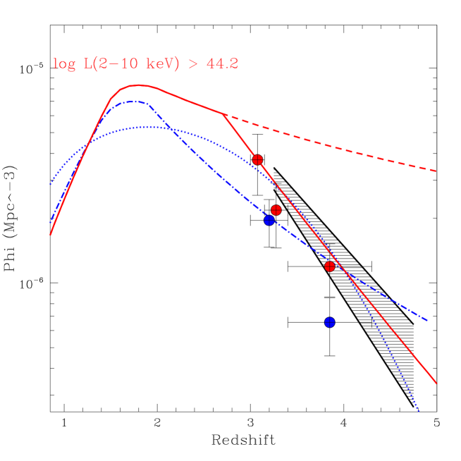
Figure 9: The comoving space density in three ($z$ = 3.0–4.5) different redshift bins for the $z>$ 3, log$L_{X}>44.2$ XMM–COSMOS sample. Red symbols (with associated errors) refer to the full sample (34 objects) and have been corrected for incompleteness against obscured sources (see text for details). The red curve corresponds to the X–ray selected AGN space density computed for the same luminosity limit from the Gilli et al. (2007) model. At $z>2.7$ we plot with two separate curves expectations when the exponential decline in the X–ray LF at $z>$ 2.7 is introduced (continuous line) or not (dashed line, see text for details). Blue symbols (and associated errors) refer to the $i<24$ sample (28 objects) and are corrected only for the volume effects to be compared with the Silverman et al. (2008) LF. The dot-dashed and dotted lines correspond to the Silverman et al. (2008) LF, in the case of the LDDE and mod-PLE model, respectively (see Silverman et al. 2008 for details). The black shaded area represents the shape derived from brighter optical quasars surveys (Schmidt et al. 1995 and Richards et al. 2006, upper and lower bounds respectively), rescaled up by an arbitrary factor $\sim 80$ for an easier comparison with the X–ray data.

In order to compare our findings with the Silverman et al. (2008) recent estimates of the high-redshift LF, we have considered the same limit they adopted in the optical magnitude ($i<24$) without correction for the incompleteness towards the most obscured sources. The blue symbols in Fig. 9 are the space densities derived from the 28 objects at $I<24$, computed correcting only for volume. The mod-PLE Silverman et al. (2008) LF is higher than our data over the entire redshift range ($3<z<4$); their LDDE LF is instead in very good agreement with our data point in the first redshift bin, while it is a factor of $\sim 2$ higher than our data at $z>3.5$.

6 Results and Discussion

The analysis of optical colors and X–ray spectra indicates that high redshift, X–ray selected QSOs have optical properties not significantly different from those of optically selected, bright QSOs, even if a non-negligible fraction ($\sim 20$% i.e. the outliers of fig. 4) would not have been selected by the Casey et al. (2008) optical color-color criteria. Not surprisingly, these sources are optically faint and make up a significant fraction (30%) of the spectroscopically unidentified objects for which the observed HR does not allow to constrain the column density.

Even if the bulk of the population of obscured AGN responsible for the X–ray background is not fully sampled at the limiting flux of the XMM–COSMOS survey, the relative fraction ($\sim$ 20%) of obscured (log$N_{H}>$ 23) QSOs is not inconsistent, given the small number statistics, with that ($\sim$ 10 %) predicted by Gilli et al. (2007). We note, moreover, that the log$N_{H}>23$ sample might be contaminated by less obscured sources (log$N_{H}=22-23$) given the relatively large errors associated to the measured HR. The depth of the XMM–COSMOS survey does not allow us to further investigate the absorption distribution for column densities lower than log$N_{H}\simeq$ 23, nor to firmly establish whether optically faint sources are X–ray obscured. The fraction of outliers in the optical color–color diagram is very similar to that of X–ray obscured sources and both are close to 20%. However, the two subsamples are marginally overlapping (only two optical outliers are also X–ray obscured) suggesting that gas absorption and dust reddening are not tightly correlated (see Maiolino et al. 2001).

The X–ray luminosity function of hard X–ray selected AGN as determined by combining several Chandra and XMM surveys (Ueda et al. 2003; La Franca et al. 2005) is well constrained up to relatively low redshifts ($z\sim$ 2–3). At higher redshifts, the number statistics has so far prevented a robust estimate of their space density. Evidence for a decline at $z>$ 3 was reported by Hasinger et al. (2005) and Silverman et al. (2005), but is limited to bright, unobscured QSOs. The $z>$ 3 QSOs sample drawn from the XMM–COSMOS survey allowed us, for the first time, to firmly address the issue of the evolution of high redshift QSOs thanks to a homogeneous and sizable sample of X–ray sources much less biased with respect to mildly obscured AGN and with an almost complete redshift information. The results indicate that the comoving space density of X–ray luminous ($L_{X}\hbox{\raise 2.15277pt\hbox{$>\lower 4.56386pt\hbox{$\kern-10.70009pt{\sim}$}$}}10^{44}$ erg s^-1) QSOs at $z\sim 3$ is ($3.7\pm 1.2)\times 10^{-6}$ Mpc^-3 and declines exponentially (by an e–folding per unit redshift) in the $z\sim$ 3.0–4.5 range. These results appear to be robust, despite the still remaining (small) uncertainties on the photometric redshifts discussed in Sect. 2.2. Moreover, if all the sources undetected in the optical band were at $z>3$ equally populating the different redshifts bins, the shape of the space density as a function of redshift would not change significantly. Only in the case that all the 10 optically undetected, soft X–ray sources turn out to be at $z>$3.5-4, the analytical parameterization of the observed decay should be modified.

The high–redshift decline is similar to that of luminous ($M_{I}<-27.6$), optically bright, unobscured QSOs as well established by SDSS observations (Richards et al. 2006) and can be satisfactorily described by the Schmidt et al. (1995) parameterization. Assuming an X–ray to optical spectral index appropriate for these luminosities ($\alpha_{\rm ox}=-1.65$, e.g.Vignali et al. 2003, Steffen et al. 2006), the absolute magnitude SDSS limit corresponds to an X–ray luminosity log$L_{X}\sim 45$. Therefore, the observed decline in the space density for the XMM–COSMOS sample strongly suggests that the evolution of mildly obscured (Compton thin) AGN is very similar to that of unobscured, optically luminous QSOs, provided that the shape of the declining function holds also for luminosities which are about an order of magnitude lower than those probed by SDSS.

Silverman et al. (2008) computed the XLF for the optically bright ($i<24$) X-ray population. Even though there is a good agreement at $z<$ 3.5 between their LDDE XLF and the observed XMM-COSMOS space densities (for the same limit in the optical magnitude), the extrapolation of their XLF at higher redshift is larger, by a factor of $\sim 2$, with respect to our data. A better fit would be obtained by tuning the Silverman et al. (2008) LF parameters responsible for the high redshift ($z>$ 3.0–3.5) behavior.

The observed decline in the comoving space density of X–ray selected QSOs, at least for luminosities larger than $\sim 10^{44}$ erg s^-1, has a significant impact on the predictions of the QSOs number counts expected from future large area X–ray surveys, and, more in general, on predictions at all the wavelengths based on the current available XLF as representative of the high-redshift, radio quiet population (e.g. Wilman et al. 2008). The present results may also provide a benchmark for theoretical models of SMBH growth. For example, the $z>$ 4 QSOs number counts predicted by the Rhook & Haehnelt (2008) models (see central and right panels in their Fig. 6) are about a factor 7–8 higher than what is actually observed, suggesting that some of the model parameters should be revised.

The predicted number counts for a model with and without an exponential decline, at different limiting fluxes and redshift ranges are listed in table 4. The Chandra-COSMOS survey provides a homogeneous coverage with high-resolution (HPD $<2^{\prime\prime}$) over the central $\sim 0.5$ deg² in COSMOS (Elvis et al. 2008) down to a limiting flux of $\sim 4\times 10^{-16}$ erg cm^-2 s^-1 in the 0.5-2 keV band (see vertical line in Fig. 8). It will therefore roughly double the number of $z>3$ quasars in that area, exploring the flux regime where the contribution from most obscured sources is higher.

As a practical example we also report the expectations for the eROSITA (extended ROentgen Survey with an Imaging Telescope Array) survey with the SRG (Spectrum Röntgen Gamma) mission , which will be launched in the next years. eROSITA will survey the entire extragalactic sky down to a limiting flux of $\sim 10^{-14}$ erg cm^-2 s^-1in the 0.5-2 keV band. The number of expected $z>3$ ($z>4$) QSOs in the all sky survey, when the decline described in $\S$5.2 is incorporated in our current knowledge of the XLF, is 2.5$\times 10^{4}$ (2100). eROSITA will also perform a deeper survey over an area of $\sim 400$ deg² down to a depth of $4\times 10^{-15}$ erg cm^-2 s^-1. We expect to reveal $\sim 2500$ QSOs at $z>3$, about 200 of them at $z>4$ and better constrain their redshift distribution.

The study of QSOs space density and evolution at lower X–ray luminosities and higher redshifts requires much deeper observations. While a few moderately luminous (log$L_{X}\sim$ 43–44), high redshift $z>$ 4 quasars are detected in deep Chandra fields (i.e. Vignali et al. 2002) the present sample size is not such to constrain their space density. Additional high–z objects are expected to be revealed by ongoing ultra-deep Chandra (Luo et al. 2008) and XMM–Newton surveys.

7 Summary

Taking advantage of the large area of the XMM–COSMOS survey and the associated deep multiwavelength follow-up, we have studied the physical and cosmological properties of $z>$ 3, X–ray selected QSOs. This sample of 40 objects constitutes the largest and most complete (in term of spectroscopic confirmation, 55%) sample of high redshift quasars published so far and extracted from a single survey, at the depth of $10^{-15}$ erg cm^-2 s^-1 in the 0.5-2 keV band.

The most important results of our analysis can be summarized as follows:

• X–ray selected QSOs have optical properties which are not significantly different from those of optically selected (i.e. SDSS) objects.

• From the analysis of X–ray colors and stacked spectra there is evidence of substantial X–ray absorption in about 20% of the sources.

• There is no clear correlation between X–ray obscured sources and outliers in the adopted optical color–color diagram; however, the outliers may contribute to the flatter X–ray spectrum observed for the spectroscopically unidentified objects sample for which the observed HR does not allow to constrain the column density.

• A steep decline in the space density of luminous X–ray selected QSOs ($L_{X}>$ 10^44.2 erg s^-1) at $z>$ 3, similar to that observed for luminous optically selected quasars, is needed to fit the observed data. This suggests that the evolution of obscured AGN is similar to that of unobscured ones.

We emphasize that, while the currently available XLF (e.g. Ueda et al. 2003, La Franca et al. 2005, Hasinger et al. 2005, Silverman et al. 2008) provide an excellent fit to the $z<3$ redshift population, their extrapolations to high redshift would overpredict the present observational constraints by a factor $\sim 2$ at $z\sim 3$ and $\hbox{\raise 2.15277pt\hbox{$>\lower 4.56386pt\hbox{$\kern-10.70009pt{\sim}$}$}}5$ at $z\sim 4$. As far as the luminous quasars are concerned (logL${}_{X}>44.2$), a decay in their space density at $z\hbox{\raise 2.15277pt\hbox{$>\lower 4.56386pt\hbox{$\kern-10.70009pt{\sim}$}$}}3$ should be included in the predictions of the high–z quasar population.

Future medium deep all sky X-ray surveys (e.g. eROSITA) with the associated multiwavelength follow–up will provide sizable samples ($>10^{4}$) of $z>3$ QSOs to further constrain the bright end of the QSOs luminosity function. The evolution of the faint end of X–ray selected QSOs luminosity function up to very high redshift, $z\sim$ 6 and perhaps beyond, will be investigated by future missions such as IXO and Generation–X.

Table 1: List and coordinates of the $z>3$ QSOs from the XMM-COSMOS sample

IAU namea	XIDb	IDc	RAd	DECd
			hh:mm:ss	dd:mm:ss
XMMC_J100101.6+023846	326	2668917	10:01:01.51	+02:38:48.68
XMMC_J100157.5+014446	2518	448852	10:01:57.72	+01:44:47.05
XMMC_J100119.9+023444	418	2289051	10:01:20.05	+02:34:43.82
XMMC_J100226.0+024611	5331	2558690	10:02:26.11	+02:46:10.78
XMMC_J100223.2+022557	10690	1849901	10:02:23.31	+02:25:58.17
XMMC_J100050.6+022328	349	1977373	10:00:50.58	+02:23:29.30
XMMC_J095755.4+022400	2407	2132709	09:57:55.47	+02:24:01.18
XMMC_J095931.8+023018	262	2421306	09:59:31.80	+02:30:18.51
XMMC_J095806.9+022248	2421	2137194	09:58:06.98	+02:22:48.59
XMMC_J095840.6+021003	5347	1749560	09:58:40.71	+02:10:03.72
XMMC_J095859.5+024356	5161	2768843	09:58:59.70	+02:43:55.25
XMMC_J100228.8+024017	5175	2583306	10:02:28.82	+02:40:17.08
XMMC_J100220.3+020452	5345	1131048	10:02:20.37	+02:04:52.91
XMMC_J100023.4+020115	469	1259457	10:00:23.24	+02:01:17.40
XMMC_J100256.8+024320	5219	2534376	10:02:56.92	+02:43:21.27
XMMC_J095740.6+025259	60311	3190185	09:57:40.70	+02:52:58.77
XMMC_J100113.3+014542	53733	485583	10:01:13.45	+01:45:41.89
XMMC_J100111.4+020853	60131	1593500	10:01:11.34	+02:08:55.84
XMMC_J100050.1+022855	180	2350265	10:00:50.12	+02:28:54.97
XMMC_J100127.5+020837	2394	1594618	10:01:27.53	+02:08:37.79
XMMC_J095928.7+021738	1151	2039436	09:59:28.72	+02:17:38.57
XMMC_J100057.8+023931	187	2665989	10:00:57.79	+02:39:32.61
XMMC_J095923.0+022853	5482	2426654	09:59:22.98	+02:28:54.03
XMMC_J100255.6+013057	60186	46132	10:02:55.81	+01:30:58.05
XMMC_J100145.6+024212	5382	2615665	10:01:45.58	+02:42:12.59
XMMC_J100256.6+021159	5116	1462117	10:02:56.53	+02:11:58.48
XMMC_J100000.9+020220	5583	1294973	10:00:01.05	+02:02:20.03
XMMC_J095901.2+024419	5162	2767217	09:59:01.29	+02:44:18.81
XMMC_J100312.0+024916	53351	2910750	10:03:12.06	+02:49:15.75
XMMC_J095753.2+024737	5199	3176366	09:57:53.49	+02:47:36.25
XMMC_J095854.2+023753	5525	2832144	09:58:54.36	+02:37:53.38
XMMC_J100232.9+022331	60007	1859446	10:02:33.23	+02:23:28.86
XMMC_J095931.0+021332	504	1694357	09:59:31.01	+02:13:33.01
XMMC_J100104.2+014202	2602	500928	10:01:04.17	+01:42:03.13
XMMC_J100050.2+022618	300	1965822	10:00:50.16	+02:26:18.48
XMMC_J100248.9+022210	5592	1864254	10:02:48.90	+02:22:12.07
XMMC_J095906.4+022638	5606	2042408	09:59:06.46	+02:26:39.50
XMMC_J095752.1+015118	5594	1061300	09:57:52.16	+01:51:20.15
XMMC_J095856.7+021047	54439	1705273	09:58:56.69	+02:10:47.75
XMMC_J100152.0+023152	5259	2260872	10:01:52.10	+02:31:55.19

Table 2: Properties of $z>3$ QSOs from the XMM-COSMOS sample

XID	zspec	zphot	i (AB)	F${}_{0.5-2~{}\rm keV}$	logL${}_{2-10~{}\rm keV}$h	HR
				10-15 erg cm-2 s-1	erg s-1
326	3.003c	3.06 (3.04-3.08)	23.23	1.21	44.05	$<-0.53$
2518	…	3.01 (2.96-3.06)a	23.96	1.31	44.26	0.17
418	…	3.03 (1.58-3.84)b,e	27.02	1.73	44.25	-0.28
5331	3.038	3.04 (3.02-3.06)	20.28	4.58	44.62	-0.59
10690	…	3.09 (3.06-3.12)	23.24	1.29	44.10	$<-0.40$
349	3.092	3.09 (3.06-3.10)	22.58	1.76	44.29	-0.23
2407	3.093	0.99 (0.96-1.02)	21.26	11.4	45.06	-0.46
262	…	3.10 (2.46-3.26)a,e	25.82	5.69	44.75	-0.50
2421	3.104	3.11 (3.08-3.12)	20.89	5.22	44.73	-0.41
5347	…	3.13 (2.60-3.24)b	24.71	2.05	44.29	$<-0.57$
5161	…	3.14 (3.10-3.18)	24.00	1.64	44.29	-0.14
5175	3.143	3.13 (3.10-3.16)	22.07	6.63	44.84	-0.44
5345	…	3.29 (3.26-3.32)	23.15	1.86	44.31	$<-0.50$
469	…	3.30 (3.14-3.40)	24.42	1.08	44.10	$<-0.40$
5219	3.304	3.25 (3.22-3.28)	22.25	2.21	44.39	$<-0.42$
60311	…	3.31 (3.28-3.34)	21.92	2.99	44.51	$<-0.11$
53733	…	3.32 (3.26-3.40)	25.02	1.00	44.07	$<-0.44$
60131	3.328d	3.47 (3.44-3.50)	20.53	1.09	44.21	0.10
180	3.333	3.34 (3.32-3.36)	20.17	2.96	44.51	$<-0.73$
2394	3.333c	3.31 (3.28-3.34)	23.16	3.37	44.61	-0.36
1151	3.345d	3.38 (3.36-3.40)	21.77	3.41	44.67	-0.08
187	3.356c	3.33 (3.30-3.36)	22.36	3.78	44.67	-0.38
5482	…	3.36 (3.34-3.38)	23.22	1.70	44.34	-0.26
60186	…	3.40 (0.22-3.42) b	22.11	2.98	44.54	$<-0.08$
5382	3.465	3.44 (3.42-3.46)	23.08	1.14	44.17	$<-0.31$
5116	…	3.47 (3.46-3.50)	20.29	4.15	44.73	-0.43
5583	3.499	3.49 (3.48-3.52)	21.88	1.48	44.28	$<-0.57$
5162	3.524e,g	3.52 (3.50-3.56)	22.93	1.92	44.45	-0.11
53351	…	3.53 (2.22-3.70) b,e	24.86	2.84	44.63	-0.04
5199	3.609	3.61 (3.58-3.62)	21.96	2.68	44.60	-0.21
5525	…	3.65 (3.62-3.66)	22.28	2.82	44.64	-0.13
60007	…	3.65 (3.62-3.68)	22.17	0.96f	44.21	0.14
504	3.651	3.65 (3.62-3.66)	22.72	1.48	44.32	$<-0.53$
2602	…	3.70 (1.42-4.04)b	24.79	1.87	44.44	$<-0.62$
300	3.715	3.54 (3.52-3.56)	21.24	1.62	44.38	$<-0.57$
5592	3.745c	3.76 (3.74-3.80)	22.47	2.21	44.52	$<-0.41$
5606	4.166e,g	4.01 (3.96-4.06)	22.79	1.33	44.42	$<-0.51$
5594	4.174	3.73 (3.70-3.74)	21.08	1.27	44.40	$<-0.28$
54439	4.241e	4.24 (4.22-4.26)	23.53	1.36	44.45	$<-0.37$
5259	…	4.45 (4.42-4.50)e	26.36	1.08	44.39	$<-0.49$

Table 3: Summary of stacking results for the $z>3$ QSOs samples

sample	# of sources	Total net counts	$\Gamma$
			simple PL
log $N_{H}<$ 23	26	1200.9	1.8${}^{+0.2}_{-0.3}$
log $N_{H}>$ 23	9	342.4	0.9${}^{+0.7}_{-0.8}$
log $N_{H}<$ 23, BL AGN	16	782.1	1.7${}^{+0.3}_{-0.3}$
log $N_{H}<$ 23, phot-z	10	418.8	1.5${}^{+0.4}_{-0.5}$

Table 4: Expected numbers of z$>3$ QSOs in 0.5-2 keV surveys

z range	limiting flux	constanta	declineb
	erg cm-2 s-1	deg-2	deg-2
$z>3$	$>4\times 10^{-16}$	230	75
	$>10^{-15}$	80	30
	$>4\times 10^{-15}$	14	6.2
	$>10^{-14}$	1.8	0.75
$z>4$	$>4\times 10^{-16}$	80	12
	$>10^{-15}$	30	7
	$>4\times 10^{-15}$	3	0.5
	$>10^{-14}$	0.6	0.07

References

- Adelman-McCarthy et al. (2005) Adelman-McCarthy, J.K., Agüeros, M.A., Allam, S.S. et al., 2006, ApJS 162, 38
- Aird et al. (2008) Aird, J., Nandra, K., Georgakakis, A., Laird, E.S., Steidel, C.C., & Sharon, C., 2008, MNRAS in press [arXiv:0804.0760]
- Alexander et al. (2001) Alexander, D.M., Brandt, W.N., Hornschemeier, A.E., Garmire, G.P., Schneider, D.P., Bauer, F.E., & Griffiths, R.E., 2001, AJ 122, 2156
- Bongiorno et al. (2007) Bongiorno, A., Zamorani, G., Gavignaud, I., et al., 2007, A&A 473, 443
- Brandt & Hasinger (2005) Brandt, N.W. & Hasinger, G., 2005, ARA&A 43, 827
- Brusa et al. (2005) Brusa, M., Comastri, A., Daddi, E., et al., 2005, A&A 432, 69
- Brusa et al. (2007) Brusa, M., Zamorani, G., Comastri, A., et al. 2007, ApJS 172, 353
- Brusa et al. (2008) Brusa, M., et al., 2008 in preparation
- Capak et al. (2007) Capak, P., Aussel, H., Ajiki, M., et al. 2007, ApJS 172, 99
- Cappelluti et al. (2007) Cappelluti, N., Hasinger, G., Brusa, M., et al., 2007, ApJS 172, 341
- Cappelluti et al. (2008) Cappelluti, N., et al., 2008, in preparation
- Casey et al. (2008) Casey, C.M., Impey, C.D., Trump, J.R., Gabor, J., Abraham, R.G., Capak, P., Scoville, N.Z., Brusa, M., & Schinnerer, E., 2008, ApJS 177, 131
- Civano et al. (2008) Civano, F., et al. 2008, in preparation
- Cocchia et al. (2007) Cocchia, F., Fiore, F., Vignali, C. et al. 2007, A&A 466, 31
- Colless et al. (2001) Colless, M., Dalton, G., Maddox, S., et al., 2001, MNRAS 328, 1039
- Croom et al. (2004) Croom, S.M., Smith, R.J., Boyle, B.J., Shanks, T., Miller, L., Outram, P.J., & Loaring, N.S., 2005, MNRAS 349, 1397
- Di Matteo et al. (2005) Di Matteo, T., Springel, V., & Hernquist, L., 2005, Nature 433, 604
- Elvis et al. (2008) Elvis, M., et al. 2008, in preparation
- Fabian & Iwasawa (1999) Fabian, A.C., & Iwasawa, K., 1999, MNRAS 303L, 34
- Fan et al. (2001) Fan, X., Strauss, M.A., Schneider, D.P., et al., 2001, AJ 121, 54
- Fan et al. (2004) Fan, X., Hennawi, J.F., Richards, G.T., et al., 2004, AJ 128, 515
- Ferrarese & Merritt (2000) Ferrarese, L., & Merrit, D., 2000, ApJ 539, L9
- Finoguenov et al. (2007) Finoguenov, A., Guzzo, L., Hasinger, G., et al. 2007, ApJS 172, 182
- Finoguenov et al. (2008) Finoguenov, A., et al. 2008 in preparation
- Fiore et al. (2003) Fiore, F., Brusa, M., Cocchia, F. et al. 2003, A&A 409, 79
- Fiore et al. (2008) Fiore, F., Grazian, A., Santini, P., et al., 2008, ApJ 672, 94
- Fontanot et al. (2007) Fontanot, F., Cristiani, S., Monaco, P., et al., 2007, A&A 461, 39
- Gallagher et al. (2002) Gallagher, S.C., Brandt, W.N., Chartas, G., & Garmire, G.P., 2002, ApJ 567, 37
- Gebhardt et al. (2000) Gebhardt, K., Kormendy, J., Ho, L., et al. 2000, ApJ 543, L5
- Gilli, Comastri & Hasinger (2007) Gilli, R., Comastri, A., & Hasinger, G. 2007, A&A 463, 69
- Hasinger, Miyaji & Schmidt (2005) Hasinger, G., Miyaji, T., & Schmidt, M., 2005, A&A 441, 417
- Hasinger et al. (2007) Hasinger, G., Cappelluti, N., Brunner, H. et al., 2007, ApJS 172, 29
- Hasinger (2008) Hasinger, G., 2008, A&A in press [arXiv:0808.0260]
- Hopkins et al. (2005) Hopkins, P.F., Hernquist, L., Martini, P., Cox, T.J., Robertson, B., Di Matteo, T., & Springel, V., 2005, ApJ 625, 71
- Hunt et al. (2004) Hunt, M.P., Steidel, C.C., Adelberger, K.L., & Shapley, A.E., 2004, ApJ 605, 625
- Kaufmann et al. (2003) Kauffmann, G., Heckman, T., Tremonti, C., et al., 2003, MNRAS 346, 1055
- Koekemoer et al. (2004) Koekemoer, A. M., Alexander, D.M., Bauer, F.E. et al. 2004, ApJ 600, L123
- Koekemoer et al. (2008) Koekemoer, A. M., et al., 2008, in preparation
- La Franca et al. (2005) La Franca, F., Fiore, F., Comastri, A., et al., 2005, ApJ 635, 864
- Lapi et al. (2006) Lapi, A., Shankar, F., Mao, J., Granato, G.L., Silva, L., De Zotti, G., & Danese, L., 2006, ApJ 650L, 42
- Leauthaud et al. (2007) Leauthaud, A., et al. 2007, ApJS 172, 219
- Lilly et al. (2007) Lilly, S.J., Le Fèvre, O., Renzini, A., et al., 2007, ApJS 172. 70
- Luo et al. (2008) Luo, B., Bauer, F.E., Brandt, W.N., et al., 2008, ApjSS, in press [arXiv:0806.3968]
- Mainieri et al. (2005) Mainieri, V., Rosati, P., Tozzi, P., et al., 2005, A&A 437, 805
- Mainieri et al. (2007) Mainieri, V., Hasinger, G., Cappelluti, N., et al., 2007, ApJS 172, 368
- Maiolino et al. (2001) Maiolino, R., Marconi, A., Salvati, M., Risaliti, G., Severgnini, P., Oliva, E., La Franca, F., Vanzi, L., 2001, A&A 365, 28
- Menci et al. (2008) Menci, N., Fiore, F., Puccetti, S., & Cavaliere, A., 2008, ApJ in press [arXiv:0806.4543]
- Merloni & Heinz (2008) Merloni, A., & Heinz, S., 2008, MNRAS 388, 1011
- Mignoli et al. (2004) Mignoli, M., Pozzetti, L., Comastri, A., et al. 2004, A&A 418, 827
- Norman et al. (2002) Norman, C., Hasinger, G., Giacconi, R., et al., 2002, ApJ 571, 218
- Prescott et al. (2006) Prescott, M.K.M., Impey, C.D., Cool, R.J., & Scoville, N.Z., 2006, ApJ 644, 100
- Puccetti et al. (2008) Puccetti, S., et al. 2008, in preparation
- Rhook & Haenelt (2008) Rhook, K.J., & Haehnelt, M.G., 2008, MNRAS in press, [arXiv:0801.3482]
- Richards et al. (2006) Richards, G., Strauss, M.A., Fan, X., et al., 2006, AJ 131, 2766
- Salvato et al. (2008) Salvato, M., Hasinger, G., Ilbert, O., et al., 2008, in preparation
- Sandage & Wyndham (1965) Sandage, A., & Wyndham, J.D., 1965, ApJ 141, 328
- Schmidt (1968) Schmidt, M., 1968, ApJ 151, 393
- Schmidt & Green (1983) Schmidt, M., & Green, R.F. 1983, ApJ 269, 352
- Schmidt, Schneider & Gunn (1995) Schmidt, M., Schneider, D.P., & Gunn, J.E., 1995, AJ 110, 68
- Scoville et al. (2007a) Scoville, N.Z., Aussel, H., Brusa, M., et al., 2007, ApJS 172, 1
- Shemmer et al. (2005) Shemmer O., Brandt W.N., Gallagher S.C., Vignali C.., Boller Th., Chartas G., & Comastri, A., 2005, AJ 130, 2522
- Siana et al. (2008) Siana, B., Polletta, M., Smith, H.E., wt al., 2008, ApJ 675, 49
- Silverman et al. (2005) Silverman, J.D., Green, P.J., Barkhouse, W. A., et al., 2005, ApJ 624, 630
- Silverman et al. (2008) Silverman, J.D., et al. 2008, ApJ 679, 118
- Taniguchi et al. (2007) Taniguchi Y., et al., 2007, ApJS 172, 9
- Taniguchi et al. (2008) Taniguchi Y., et al., 2008, in preparation
- Tozzi et al. (2006) Tozzi, P., Gilli, R., Mainieri, V., et al., 2006, A&A 451, 457
- Treister & Urry (2005) Treister, E., & Urry, C.M., 2005, ApJ 630, 115
- Treister & Urry (2006) Treister, E., & Urry, C.M., 2006, ApJ 652L, 79
- Trump et al. (2007) Trump, J.R., Impey, C.D., McCarthy, P.J., et al. 2007, ApJS172, 383
- Trump et al. (2008) Trump, J.R., Impey, C.D., Elvis, M., et al. 2008, in preparation
- Ueda et al. (2003) Ueda, Y., Akiyama, M., Ohta, K., & Miyaji, T., 2003, ApJ 598, 886
- Vignali et al. (2002) Vignali, C., Bauer, F.E., Alexander, D.M., Brandt, W.N., Hornschemeier, A.E., Schneider, D.P., Garmire, G.P., 2002, ApJ 580, L105
- Vignali, Brandt & Schneider (2003) Vignali, C., Brandt, W.N., & Schneider, D.P., 2003, AJ 125, 433
- Volonteri & Rees (2006) Volonteri, M., & Rees, M., 2006, ApJ 650, 669
- Wilman et al. (2008) Wilman R.J., et al., 2008, submitted to MNRAS
- Wolf et al. (2003) Wolf, C., Meisenheimer, K., Kleinheinrich, M., et al., 2004, A&A 421, 913
- Wolf et al. (2004) Wolf, C., Wisotzki, L., Borch, A., Dye, S., Kleinheinrich, M., Meisenheimer, K., 2003, A&A 408, 499