The Parallelometer: a mechanical device to study curvature

The Parallelometer: a mechanical device to study curvature

Abstract

A simple mechanical device is introduced, the parallelometer, that can be used to measure curvatures of surfaces. The device can be used as a practical illustration of parallel transport of a vector. Its connection to the Foucault pendulum is discussed.

I Introduction

It is intuitively obvious how to transport a vector in a plane in such a way that it remains unchanged: just pick a set of cartesian coordinates and ask that the components of the vector remain constant as it is transported. As it is transported, the vector remains parallel to its initial direction in the plane. How about in a curved surface? This problem was first addressed by Levi-Civita in 1917levy who introduced the influential idea of parallel transport, later to be used extensively in the General Theory of Relativity. To parallel transport a vector along a path on a (two–dimensional) curved surface, we can first refer it to a local cartesian system which in turn has to be parallel transported. The $z$ axis is always normal to the surface. Qualitatively, the prescription of transport is that, as one moves along the curve, the $xy$ plane cannot “rotate” around the $z$ axis. A vector will be parallel transported when its components with respect to these $xy$ axes don’t change. A non-trivial result emerges: if the vector is parallel-transported around a closed curve, it returns rotated with respect to the initial orientation.

In this paper we present a simple mechanical device that measures parallel transport and can be used as a pedagogical tool. Here the phase factor in the parallel transport becomes very clear and easy to observe and study quantitatively. In principle an experiment should be easy and inexpensive and can be carried out in a basic laboratory setting, adequate for beginner or intermediate students. The system we devised, the parallelometer, consists in general of two concentric rings constrained to rotate without friction in the same plane. Consider the inner ring carried along a path maintaining its plane tangent to the surface. Since the outer ring is free to rotate, a vector connecting the center of the parallelometer to a point in the outer ring will be parallel transported along the path.bicycle The practical realizations could be a ball bearing or a freewheel.

II The Parallelometer

II.1 Lagrangian treatment

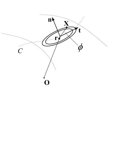
Figure 1: The parallelometer consists of a frictionless freewheel which is restricted to move along a given surface with its axis pointing along the local normal to the surface. This device will be transported along a curve $C$ on a surface $S$.

In this section we discuss the system dynamics and show that it corresponds to parallel transport. The parallelometer, consists of a frictionless freewheel which is restricted to move along a given surface with its axis pointing along the local normal to the surface This device will be transported along a curve $C$ on a surface $S$. (See Fig. 1). In this process the parallelometer is constrained to move with its plane always tangent to the surface and to move along the curve $C$. For concreteness we can think of an arrow attached to the axis of the freewheel (and perpendicular to the axis) that always points along the curve $C$.

The coordinate of a point X within the wheel, of radius $r_{0}$, is

$$\textbf{X}=\textbf{r}+r_{0}\left[\cos\beta{\textbf{t}}+\sin\beta(\textbf{n}\times{\textbf{t}})\right],$$ (1)

where t is a unit vector in the direction of the local tangent to the curve $C$ along which the parallelometer is transported. The unit vector n is the local normal to the plane tangent to the surface, and r is the coordinate of the center of the wheel. Notice that, with these definitions, the unit vectors t and $\textbf{n}\times{\textbf{t}}$ are along the natural $x$ and $y$ axis for an observer on an “inner ring” defined as the intersection of the (cylindrical) axis of the freewheel with the tangent plane. The vector n is along the corresponding $z$ axis. This frame is similar to the standard Frenet frame associated with a curve that is often used in differential geometry.spivak However, it is not identical to a Frenet frame, since its construction depends not on the curve alone but also on the surface.

The velocity of that point on the free wheel is:

$$\dot{\textbf{X}} = \dot{\textbf{r}}+r_{0}\bigl{\{}\dot{\beta}\left[-\sin\beta{\textbf{t}}+\cos\beta(\textbf{n}\times{\textbf{t}})\right]+\cos\beta\dot{{\textbf{t}}}$$ (2)

$$+ \sin\beta(\dot{{\textbf{n}}}\times{\textbf{t}}+\textbf{n}\times\dot{{\textbf{t}}})\bigr{\}}$$

Squaring $\dot{\textbf{X}}$ and integrating over $\beta$ we obtain the kinetic energy of the ring. The Lagrangian is therefore

$$L={\frac{M}{2\pi}}\int_{0}^{2\pi}d\beta\;\dot{\textbf{X}}^{2}$$ (3)

Using

$$\int_{0}^{2\pi}d\beta\,\sin\beta\cos\beta=0,$$

$$\int_{0}^{2\pi}d\beta\,\sin^{2}\beta=\int_{0}^{2\pi}d\beta\,\cos^{2}\beta=\pi$$ (4)

we obtain the corresponding Lagrangian:

$$L={\frac{1}{2}}M\dot{\textbf{r}}^{2}+{\frac{1}{2}}Mr_{0}^{2}\dot{\beta}^{2}+Mr_{0}^{2}\left[\dot{{\textbf{t}}}\cdot(\textbf{n}\times{{\textbf{t}}})\,\dot{\beta}\right]+L^{\prime}$$ (5)

where $L^{\prime}$ is a term that does not contain $\beta$ or $\dot{\beta}$ and therefore does not affect the dynamics of the angle $\beta$. Notice that the term $r_{0}\dot{{\textbf{t}}}\cdot(\textbf{n}\times{{\textbf{t}}})$ plays the role of a “gauge potential” affecting the motion of $\beta$.

The equation of motion of $\beta$ is

$${\frac{d}{dt}}{\frac{\partial L}{\partial\dot{\beta}}}={\frac{\partial L}{\partial\beta}},$$ (6)

and, since $L$ is independent of $\beta$ we have

$${\frac{\partial L}{\partial\dot{\beta}}}=\rm{Const},$$ (7)

or

$$\dot{\beta}+\dot{{\textbf{t}}}\cdot(\textbf{n}\times{{\textbf{t}}})=\rm{Const}.$$ (8)

If, as an initial condition we choose $\dot{\beta}=0$ and $\dot{{\textbf{t}}}=0$ then Const$=0$ and we obtain

$$\dot{\beta}+\dot{{\textbf{t}}}\cdot(\textbf{n}\times{{\textbf{t}}})=0,$$ (9)

We will now show that this dynamics corresponds to parallel transport provided the initial condition corresponds to Const$=0$.

II.2 Connection with parallel transport

Consider now transporting a unit vector u along the same curve $C$. Following the previous discussion, we can define a local coordinate system with the unit vectors $(\textbf{t},\textbf{n}\times{\textbf{t}},\textbf{n})$. Notice that this a cartesian system natural for an observer that faces along the direction of the motion on the curve and not the coordinate system that is parallel transported. Since the vector is always in the plane tangent to the surface we need only one coordinate to specify it in this coordinate system. We use the angle $\beta$ that the vector makes with the tangent t to the curve. This means that u can be expressed in the following way in terms of the local coordinates:

$${{\textbf{u}}}=\cos\beta{\textbf{t}}+\sin\beta(\textbf{n}\times{\textbf{t}}).$$ (10)

Now multiply the above equation by t and, using ${\textbf{t}}\cdot(\textbf{n}\times{\textbf{t}})=0$, compute the time derivative. Since

$${\textbf{t}}\cdot\textbf{u}=\cos\beta,$$ (11)

we have

$$-\dot{\beta}\sin\beta = {\frac{d}{dt}}{\textbf{u}}\cdot{\textbf{t}}$$ (12)

$$= \dot{{\textbf{u}}}\cdot{\textbf{t}}+{{\textbf{u}}}\cdot\dot{{\textbf{t}}}$$

For parallel transport of a vector two conditions have to be satisfied. First, the vector has to stay in the plane tangent to the surface. This condition is guaranteed by the form of Eq. (10). The second condition is that any variation of the vector transported is out of the plane. These two conditions combined contain the prescription for how to parallel transport a vector. The second condition in this case means

$$\dot{{\textbf{u}}}\cdot{\textbf{t}}=0,$$ (13)

so that, from (12)

$$-\dot{\beta}\sin\beta={{\textbf{u}}}\cdot\dot{{\textbf{t}}}.$$ (14)

Replacing (10) in the above equation, and using ${\textbf{t}}\cdot\dot{{\textbf{t}}}=0$ (the variation of a vector of constant length is always perpendicular to the vector) we obtain

$$-\dot{\beta}=\dot{{\textbf{t}}}\cdot(\textbf{n}\times{{\textbf{t}}})$$ (15)

which is the same as (9), obtained from dynamical considerations. The parallelometer therefore measures parallel transport provided it is started at rest.

II.3 Connection with Foucault’s pendulum

Consider the above results specified to a spherical surface and the curve $C$ being a parallel. In spherical coordinates, where $\theta$ is the polar angle and $\phi$ the asymuthal angle, we have

$${\textbf{t}}=\textbf{e}_{\phi},$$ (16)

$${\dot{{\textbf{t}}}}=-\left(\sin\phi\hat{\textbf{i}}+\cos\phi\hat{\textbf{j}}\right)\dot{\phi},$$ (17)

and

$$\textbf{n}\times{{\textbf{t}}}=-\cos\theta\left(\sin\phi\hat{\textbf{i}}+\cos\phi\hat{\textbf{j}}\right)+\sin\theta\hat{\textbf{k}},$$ (18)

where $\theta=\pi/2-\lambda$ is complementary to the latitude $\lambda$. This implies, from (15)

$$\dot{\beta}=-\cos\theta\dot{\phi},$$ (19)

or equivalently

$$d{\beta}=-\cos\theta d{\phi}.$$ (20)

Integrating over $2\pi$ we obtain

$$\Delta{\beta}\equiv\delta=-2\pi\cos\theta.$$ (21)

which is the equation for Foucault’s pendulum.

References

- (1) T. Levi-Civita, “Nozione di parallelismo su di una varietà qualunque e conseguente specificazione geometrica della curvatura riemaniana”, Rend. Circ. Mat. Palermo, 42, pp. 173–205 (1917)
- (2) M. Levi, “A ‘bicycle wheel’ proof of the Gauss-Bonnet theorem” Expo. Math. 12, 145–164 (1994)
- (3) M. Spivak, A Comprehensive Introduction to Differential Geometry, (Second Edition). Publish or Perish, Inc. Houston, Texas, (1979), Vol. 2, Chap. 1
- (4) J. von Bergmann and HsingChi von Bergmann, “Foucault pendulum through basic geometry”, Am. J. Phys., 75(10), 888-892 (2007)
- (5) J. B Hart, R. E. Miller and R. I. Mills, “ A simple geometric model for visualizing the motion of a Foucault pendulum”, Am. J. Phys., 55(1), 67-70 (1985)
- (6) Belfield-Lefebre, “Revue scientifique et industrielle”,1 (4ème sér.) pp. 19-21 (1852).
- (7) R. P. Feynman, R. B. Leighton, and M. Sands, Feynman Lectures on Physics Addison - Wesley, Reading, MA, 1970, Vol. 2, Chap. 15.