An exotic T₁S⁴ with positive curvature

Abstract.

We construct a metric with positive sectional curvature on a 7-manifold which supports an isometry group with orbits of codimension 1. It is a connection metric on the total space of an orbifold 3-sphere bundle over an orbifold 4-sphere. By a result of S. Goette, the manifold is homeomorphic but not diffeomorphic to the unit tangent bundle of the 4-sphere.

Spaces of positive curvature play a special role in geometry. Although the class of manifolds with positive (sectional) curvature is expected to be relatively small, so far there are only a few known obstructions. Moreover, for closed simply connected manifolds these coincide with the known obstructions to nonnegative curvature which are: (1) the Betti number theorem of Gromov which asserts that the homology of a compact manifold with non-negative sectional curvature has an a priori bound on the number of generators depending only on the dimension, and (2) a result of Lichnerowicz and Hitchin implying that a spin manifold with non-trivial $\hat{A}$ genus or generalized ${\mathfrak{a}}$ genus cannot admit a metric with non negative curvature.

One way to gain further insight is to construct and analyze examples. This is quite difficult and has been achieved only a few times. Aside from the classical rank one symmetric spaces, i.e., the spheres and the projective spaces with their canonical metrics, and the recently proposed deformation of the so-called Gromoll-Meyer sphere [PW2], examples were only found in the 60’s by Berger [Be], in the 70’s by Wallach [Wa] and by Aloff and Wallach [AW], in the 80’s by Eschenburg [E1, E2], and in the 90’s by Bazaikin [Ba]. The examples by Berger, Wallach and Aloff-Wallach were shown, by Wallach in even dimensions [Wa] and by Berard-Bergery [BB] in odd dimensions, to constitute a classification of simply connected homogeneous manifolds of positive curvature, whereas the examples due to Eschenburg and Bazaikin typically are non-homogeneous, even up to homotopy. All of these examples can be obtained as quotients of compact Lie groups $G$ with a biinvariant metric by a free isometric “two sided” action of a subgroup $H\subset G\times G$. Since a Lie group with a biinvariant metric has nonnegative curvature so do such quotients, and in rare cases one even gets positive curvature. To achieve this no further curvature computations are required, it suffices to show that any horizontal 2-plane, when translated back to the identity in $G$, cannot contain two vectors whose Lie bracket is $0$. See [Zi1] for a survey of the known examples.

Our main purpose here is to present a new method for the construction of positively curved manifolds, and to use it to exhibit one new manifold with positive curvature (see [De2] for an independent and different approach):

Theorem A.

There is a positively curved 7-manifold, which is homeomorphic, but not diffeomorphic to the unit tangent bundle of the 4-sphere.

Our result is actually stronger than stated: We exhibit an explicit metric $g$ and a 4-form $\eta$, and prove that the modified curvature operator $\hat{R}+\hat{\eta}$ on the bundle of 2-forms (automatically having the same “sectional curvatures”) is positive. Recall that $\hat{R}$ itself being positive is extremely strong and only can happen for manifolds diffeomorphic to space forms [BW]. The idea to consider such modified curvature operators was pioneered by Thorpe in dimension 4, and implemented in higher dimensions by Püttmann [Pü], where it was shown that all homogeneous positively curved metrics have strongly positive curvature in this sense. It is the first time, however, that this method has been used to establish positivity of curvature in a new example.

The example is indeed a new one, since $T_{1}\mathbb{S}^{4}$ is 2-connected with third homotopy group ${\mathbb{Z}}_{2}$, and the only other known 2-connected positively curved 7-manifolds are $\mathbb{S}^{7}$ and the Berger space $B^{7}=\operatorname{SO}(5)/\operatorname{SO}(3)$ with $\pi_{3}(B^{7})={\mathbb{Z}}_{10}$ [Be]. It is a highly non-trivial and recent result due to S. Goette [G] that our new example is diffeomorphic to a 3-sphere bundle over the 4-sphere, and is homeomorphic but not diffeomorphic to $T_{1}\mathbb{S}^{4}$ (see [CE],[KS], and [Cr] for a proof that they are homeomorphic). Furthermore, from [KZ],[To], it follows that it is not diffeomorphic to any biquotient. We point out that it is not yet known if $T_{1}\mathbb{S}^{4}$ itself has a metric of positive curvature, but P.Petersen and F.Wilhelm have shown that it supports a metric with positive curvature on an open and dense set [PW1].

Our example, is the second among an explicitly given infinite sequence $\{P_{k}\},k=1,2,\ldots$ of 2-connected cohomogeneity one $\operatorname{SO}(4)$ 7- manifolds with $\pi_{3}(P_{k})={\mathbb{Z}}_{k}$ for which no obstructions to positive curvature are known (cf. [GWZ]), the first being $P_{1}=\mathbb{S}^{7}$. By construction, the subaction by $\operatorname{S}^{3}\subset\operatorname{SO}(4)$ on $P_{k}$ also yields the structure of an orbifold principle $\operatorname{S}^{3}$- bundle over $\mathbb{S}^{4}$, and our metric on $P_{2}$ is an orbifold connection metric for this bundle. Here the orbifold setting is crucial, since it is well known that a connection metric on a smooth $\mathbb{S}^{3}$ bundle over $\mathbb{S}^{4}$ has positive curvature only in the case of the Hopf bundle, where the total space is $\mathbb{S}^{7}$, [DR].

In general, the attempt to describe and eventually classify positively curved manifolds with large isometry group provides a natural framework for a systematic search for new examples ( see [Gr],[Wi2]). The manifold $P_{2}$ has indeed emerged in this context: Specifically, in [V1, V2] and [GWZ] an exhaustive description was given of all simply connected cohomogeneity one manifolds that can possibly support an invariant metric with positive curvature. In addition to the normal homogeneous manifolds of positive curvature and a subset among the Eschenburg and Bazaikin spaces which admit a cohomogeneity one action, two infinite families, $P_{k},Q_{k}$ and one exceptional manifold $R$, all of dimension seven (with ineffective actions of $\operatorname{S}^{3}\times\operatorname{S}^{3}$), appeared as the only possible new candidates (see [GWZ] and the survey [Zi2]). Here $Q_{1}$ is the normal homogeneous positively curved Aloff-Wallach space ([Wi1]). Recently it was shown in [VZ2] that the exceptional candidate $R$ in fact does not admit an invariant metric with positive curvature.

It is a curious fact, as was proved in [GWZ], that the infinite families admit a different description: They are the two-fold universal covers, $P_{k}\to H_{2k-1}$ and $Q_{k}\to H_{2k}$ of the frame bundle $H_{\ell}$ of self-dual 2-forms associated to the self dual Einstein orbifolds $O_{\ell}$ ($\mathbb{S}^{4}$ with an $\operatorname{SO}(3)$ invariant orbifold metric) constructed by Hitchin in [Hi1]. As such, these manifolds come with natural 3-Sasakian metrics, that in particular are (orbifold) connection metrics. There is a general necessary and sufficient condition for a connection metric to have positive curvature once the fiber is shrunk sufficiently (see [CDR]), that also applies in the orbifold context. In the special case of 3-Sasakian metrics this is equivalent to the base having positive curvature. Unfortunately the curvature of the Hitchin metrics are positive only for $O_{1}$ and $O_{2}$. However, on $O_{3}$ (the base of $P_{2}$) this metric has positive curvature on a large region and only relatively small negative curvature , see Figure 8 in [Zi2]. This suggests that it might be possible to make a small change of the Hitchin metric on $O_{3}$ with positive curvature, choose a principal connection close to the Hitchin connection, and get positive curvature on the total space after shrinking the metric on the fiber sufficiently. We use the Hitchin metric and connection as a guide only. Our metric on the base, and the principal connection, are explicitly given by polynomials. For this we divide the interval on which the metric is defined into three subintervals, two close to the singular orbits, and a larger one in the middle. Near the singular orbits we find functions consisting of polynomials of degree $3$. In the middle we glue with the unique polynomials of degree $5$ such that the resulting metric on the manifold is $C^{2}$ (See (4.4) and (4.16) for the explicit formulas). It is then obvious that any smooth $C^{2}$ perturbation will have positive curvature as well. To prove that our metric has positive curvature (on each piece), the crucial and non-trivial point is to find and add an invariant 4-form so as to make the modified curvature operator positive definite when the fiber metric is shrunk sufficiently. To prove positive definiteness, given our choices, boils down to checking that specific polynomials with integer coefficients have no zeroes on a particular closed interval. This is done by using Sturm’s theorem, which counts real zeroes of such polynomials by computing the $\gcd$ of the polynomial and its derivative (i.e. applying the Euclidean algorithm).

The metric by O.Dearricott in [De2] differs from ours in that he deforms the self dual Hitchin metric on the base of the orbifold bundle conformally, but keeps the principal connection as the one coming from the Hitchin metric.

It is a natural conjecture that all the manifolds $P_{k}$ and $Q_{k}$ admit invariant metrics of positive curvature. This would be particularly interesting for the $P_{k}$ family, since they are all 2-connected, hence contradicting a conjecture in [FR]. This requires a more drastic change of the Hitchin metrics on the base and hence difficulty in a natural choice of principal connection using our method. It is not difficult to construct invariant metrics of positive curvature on the base (using, e.g., Cheeger deformations), but corresponding choices of principal connections will require new insights. We point out that the class of connection metrics, while simpler to work with geometrically, is considerably smaller than the class of general invariant metrics. In particular, we will show that the manifold $B^{7}$, although it admits a cohomogeneity one metric with positive curvature, does not admit a connection metric with positive curvature.

Here is a short description of the individual sections. In Section 1 we describe the $P_{k}$ as well as the $Q_{k}$ families including all invariant metrics on them in terms of functions on the orbit space interval. The imposed boundary conditions for these functions and general curvature formulas are easily obtained and described in the Appendix. Section 2 is devoted to a discussion of connection metrics in our context and the corresponding simplified curvature formulas and smoothness conditions. A discussion of the Thorpe method and how to choose a suitable invariant 4-form is discussed in Section 3, and Section 4 describes the metric and the principal connection. The proof that the constructed metric and chosen 4-form has positive definite “curvature operator” is carried out in Section 5.

The present paper is a minor modification of [GVZ], first made available on the arXiv with a different title.

It is a pleasure to thank Burkhard Wilking for helpful discussions and Peter Storm for suggesting the use of Sturm’s theorem in our proof. The second and third named author were also supported by IMPA in Rio de Janeiro and would like to thank the Institute for its hospitality.

1. Candidates and their invariant metrics

To establish notation, we begin with a brief review of the basic description of cohomogeneity one manifolds and their invariant metrics (for more details, we refer to [AA, GZ1, GWZ]).

Let $G$ be a compact Lie group which acts isometrically on a compact Riemannian manifold $M$ with orbit space an interval. The interior points of the interval correspond to the principal orbits, and the end points to the non-principal orbits $B_{\pm}$ (singular in the case of simply connected $M$). Let $c:[0,L]\to M$ be a distance minimizing geodesic parameterized by arclength connecting the non-principal orbits. The isotropy group at $c(0)$ is denoted by $K^{\scriptscriptstyle{-}}$ and the one at $c(L)$ by $K^{\scriptscriptstyle{+}}$. The principal isotropy group, constant for $c(t),0<t<L$, is denoted by $H$. Since the boundary of tubes around the singular orbits must be regular orbits, we have that $K^{\scriptscriptstyle{\pm}}/H$ are spheres.

An important property of cohomogeneity one manifolds is that a converse also holds: If we have compact groups with inclusions $H\subset\{K^{\scriptscriptstyle{-}},K^{\scriptscriptstyle{+}}\}\subset G$ satisfying $K^{\scriptscriptstyle{\pm}}/H=\mathbb{S}^{\ell_{\pm}}$, then one can define a cohomogeneity one manifold by gluing the two disc bundles $G\times_{K^{\scriptscriptstyle{-}}}\mathbb{D}^{\ell_{-}+1}$ and $G\times_{K^{\scriptscriptstyle{+}}}\mathbb{D}^{\ell_{+}+1}$ along their common boundary $G/H$ via the identity. One possible description of our manifold is thus simply in terms of the diagram of groups $H\subset\{K^{\scriptscriptstyle{-}},K^{\scriptscriptstyle{+}}\}\subset G$.

To describe a $G$ invariant metric on $M$, it suffices to describe the metric along $c$. For $0<t<L$, $c(t)$ is a regular point with constant isotropy group $H$ and the metric on the principal orbits $Gc(t)=G/H$ is a smooth family of homogeneous metrics $g_{t}$. Thus on the regular part the metric $\langle\ ,\ \rangle_{c(t)}=g_{c(t)}$ is determined by

$$g_{c(t)}=d\,t^{2}+g_{t},$$

and since the regular points are dense it also describes the metric on $M$. In terms of a fixed biinvariant inner product $Q$ on the Lie algebra ${\mathfrak{g}}$ and corresponding $Q$-orthogonal splitting ${\mathfrak{g}}={\mathfrak{h}}\oplus{\mathfrak{m}}$ we have $\operatorname{Ad}(H)({\mathfrak{m}})\subset{\mathfrak{m}}$ and the tangent space to $G/H$ at $c(t),t\in(0,L)$ is identified with ${\mathfrak{m}}$ via action fields: $X\in{\mathfrak{m}}\to X^{*}(c(t))$. With this terminology the metric $g_{t}$ is an $\operatorname{Ad}(H)$-invariant inner product on ${\mathfrak{m}}$. In terms of $Q$ we also have the representation

$$g_{t}(X^{*},Y^{*})=Q(P_{t}(X),Y)$$

where $P_{t}:{\mathfrak{m}}\to{\mathfrak{m}}$ is a positive, symmetric $\operatorname{Ad}(H)$ equivariant operator for each $t\in(0,L)$. When extended to the closed interval $0\leq t\leq L$, $g_{t}$ degenerates at the end points, and smoothness of the metric on $M$, correspond to explicit boundary conditions for $g_{t}$ at $0$ and at $L$ imposed by invariance (cf. [BH],[EW]).

We will now recall the explicit description of our specific candidates from [GWZ] in terms of group diagrams as above, and use it to describe all smooth invariant metrics on them.

Metrics on the $P$ family.

Regarding $\operatorname{S}^{3}$ as the unit quaternions, the group diagram for $P_{k}$ is given by:

(1.1) $$H=\Delta Q\subset\{(e^{i\theta},e^{i\theta})\cdot H\,,(e^{j(1+2k)\theta},e^{j(1-2k)\theta})\cdot H\}\subset\operatorname{S}^{3}\times\operatorname{S}^{3},$$

where $H$ is isomorphic to the quaternion group $Q=\{\pm 1,\pm i,\pm j,\pm k\}$, embedded diagonally in $\operatorname{S}^{3}\times\operatorname{S}^{3}$. The signs of these slopes differ from the ones in [GWZ], but do not affect the equivariant diffeomorphism type since we can conjugate all groups by $(1,i)$. This change simplifies the smoothness conditions.

Since $H$ is finite in our case, ${\mathfrak{m}}={\mathfrak{h}}^{\perp}={\mathfrak{g}}$ with the notation above. For a basis of ${\mathfrak{g}}$ we let $X_{i}$ and $Y_{i}$ be the left invariant vector fields on $\operatorname{S}^{3}\times\operatorname{S}^{3}$ corresponding to $i,j$ and $k$ in the Lie algebras of the first and second $\operatorname{S}^{3}$ factor of $G$. The adjoint action of $H$ is in our case by sign changes in the basis vectors $X_{i},Y_{i}$. For example, $\operatorname{Ad}(i,i)$ fixes $X_{1}$ and $Y_{1}$ and multiplies $X_{2},Y_{2},X_{3},Y_{3}$ by $-1$, and similarly for $(j,j),(k,k)\in H$. This implies in particular that

$$\langle X^{*}_{i},X^{*}_{j}\rangle=\langle X^{*}_{i},Y^{*}_{j}\rangle=\langle Y^{*}_{i},Y^{*}_{j}\rangle=0\text{ for all }i\neq j$$

The metric is therefore described by 9 functions:

(1.2) $$f_{i}(t)=\ \langle X^{*}_{i},X^{*}_{i}\rangle_{c(t)}\quad,\quad g_{i}(t)=\ \langle Y^{*}_{i},Y^{*}_{i}\rangle_{c(t)}\quad,\quad h_{i}(t)=\langle X^{*}_{i},Y^{*}_{i}\rangle_{c(t)}$$

all defined on $[0,L]$.

Metrics on the $Q$ family.

For completeness, we now shortly discuss the second family of candidates. The group diagram for $Q_{k}$ is given by

(1.3) $$H\simeq{\mathbb{Z}}_{2}\oplus{\mathbb{Z}}_{4}=\{(\pm 1,\pm 1),(\pm i,\pm i)\}\subset\{(e^{i\theta},e^{i\theta})\cdot H\,,(e^{j(k+1)\theta},e^{-jk\theta})\cdot H\}\subset\operatorname{S}^{3}\times\operatorname{S}^{3}.$$

We point out that in this case, since $H$ is smaller than for $P_{k}$, a general cohomogeneity one metric can have other non-zero inner products of the basis vectors $X_{i},Y_{i}$, but the curvature formulas in the general case are significantly more complicated. Moreover, metrics lifted from the corresponding ${\mathbb{Z}}_{2}$ quotients $H_{\ell}$ are of the above form.

Additional strong restrictions on the functions defining the metric on $P_{k}$ or $Q_{k}$ are imposed at the end points of the interval $[0,L]$, where the principal orbits collapse and is carried out for our candidates in the Appendix (see Theorem 6.1). The curvature tensor of a general cohomogeneity one metric on $P_{k}$ and $Q_{k}$ is easily obtained from known formulas and is discussed in the Appendix as well (see Theorem 6.6).

2. Connection Metrics

We now restrict our general type of cohomogeneity one metrics to so-called connection metrics. This will simplify the curvature formulas significantly (in particular when the vertical part of the metric is scaled by $\epsilon$), but also enables one to understand the behavior of the functions in a more geometric fashion.

In general, when $G$ contains a normal subgroup $L\triangleleft G$ which acts freely (or almost freely) on $M$ the quotient map $\pi:M\to M/L$ is a principal (orbifold) $L$ bundle over the $G/L$ cohomogeneity one (orbifold) base $B=M/L$. In this case, a subfamily of invariant metrics are connection metrics, i.e., metrics of the form

(2.1) $$\langle U,V\rangle=g_{B}(\pi_{*}(U),\pi_{*}(V))+Q(\theta(U),\theta(V))$$

where $g_{B}$ is a ($G/L$ invariant) metric on the base $B$, $Q$ a bi-invariant metric on ${\mathfrak{l}}$, and $\theta$ a (G invariant) connection, i.e., an invariant choice of a complement to the tangent spaces of the $L$-orbits. Note that one gets a natural family of such metrics simply by scaling $Q$ by $\epsilon$.

In our case, the above discussion applies to $L=\operatorname{S}^{3}\times\{1\}\subset\operatorname{S}^{3}\times\operatorname{S}^{3}=G$. Indeed, since $L$ is a normal subgroup of $G$, the isotropy groups of $L$ are simply the intersection of $L$ with the isotropy groups along $c(t)$. For $P_{k}$ the isotropy groups are hence trivial on $B_{-}$ and the principal orbits, and along $B_{+}$ equal to $\{e^{j(1+2k)\theta}\mid e^{j(1-2k)\theta}=1\}\simeq{\mathbb{Z}}_{2k-1}$. We thus have an orbifold principal $\operatorname{S}^{3}$ bundle, $\pi:P_{k}\to P_{k}/\operatorname{S}^{3}\times\{1\}=B$. The base $B$ carries a cohomogeneity action induced by $\{1\}\times\operatorname{S}^{3}$ since it commutes with $L$. Its isotropy groups are $e^{i\theta}\cdot H\ ,\ e^{j\theta}\cdot H\ ,$ where $H=\{\pm 1,\pm i,\pm j,\pm k\}$. This action is ${\mathbb{Z}}_{2}$ ineffective, and the corresponding effective action by $\operatorname{SO}(3)$ is in fact the remarkable cohomogeneity one action on $\mathbb{S}^{4}$, whose extension to ${\mathbb{R}}^{5}$, viewed as the symmetric traceless $3\times 3$ matrices, is by conjugation, see e.g. [GZ1]. Each of the two singular orbits are the so-called Veronese surfaces $\mathbb{R\mkern 1.0muP}^{2}\subset\mathbb{S}^{4}$. The metric on $B$ is smooth except along the right singular orbit $B_{+}/\operatorname{S}^{3}=\mathbb{R\mkern 1.0muP}^{2}$ where the “normal bundle” has fibers that are Euclidean cones over circles of length $2\pi/(2k-1)$.

Similarly, from the isotropy groups of the $\operatorname{S}^{3}\times\operatorname{S}^{3}$ action on $Q_{k}$ in (1.3), it again follows that $\operatorname{S}^{3}\times\{1\}\subset\operatorname{S}^{3}\times\operatorname{S}^{3}$ acts almost freely with isotropy groups along $B_{+}$ equal to $\{e^{j(k+1)\theta}\mid e^{jk\theta}=1\}\simeq{\mathbb{Z}}_{k}$, and trivial otherwise. In this case, the base $Q_{k}/\operatorname{S}^{3}\times\{1\}$ has an induced action by $\operatorname{S}^{3}$ with isotropy groups $e^{i\theta}\cdot H\ ,\ e^{j\theta}\cdot H\ ,$ where $H=\{\pm 1,\pm i\}$. This action is again ${\mathbb{Z}}_{2}$ ineffective and the induced action by $\operatorname{SO}(3)$ has the same isotropy groups as the action of $\operatorname{SO}(3)\subset\operatorname{SU}(3)$ on $\mathbb{C\mkern 1.0muP}^{2}$, see e.g. [Zi2]. The metric on the base $\mathbb{C\mkern 1.0muP}^{2}$ is also smooth everywhere in this case, except along the right singular orbit where the normal spaces are cones on circles of length $2\pi/k$.

To make the discussion of $P_{k}$ and $Q_{k}$ more uniform, we can further compose the projection $\pi:Q_{k}\to Q_{k}/\operatorname{S}^{3}\times\{1\}=\mathbb{C\mkern 1.0muP}^{2}$ with the two fold branched cover $\mathbb{C\mkern 1.0muP}^{2}\to\mathbb{S}^{4}$ obtained orbitwise from the respective $\operatorname{SO}(3)$ actions. From the above description of the isotropy groups of these actions one sees that this is a 2-fold cover along the principal orbits and the left hand side singular orbit. But along the right hand side singular orbit it is a diffeomorphism, which can thus be considered to be the branching locus. Orthogonal to this singular orbit it divides angles by $2$. Thus we can also regard $Q_{k}$ as an orbifold principal bundle over $\mathbb{S}^{4}$ with angle normal to $B_{+}$ equal to $2\pi/(2k)$. As we will see shortly, we will then be able to deal with $P_{k}$ and $Q_{k}$ at the same time.

We now claim that the cohomogeneity one metrics from Section 1 with

$$f=f_{i}:=\ \langle X^{*}_{i},X^{*}_{i}\rangle\quad\text{all \emph{constant} and equal }$$

in fact are connection metrics for the principal $L$-bundle $\pi\colon M\to B$. Indeed, the horizontal space is invariant under $L$ by definition. For inner products along orbits we have $\langle A^{*},B^{*}\rangle_{g\pi(c(t))}=\langle\operatorname{Ad}(g^{-1})A,\operatorname{Ad}(g^{-1})B\rangle_{\pi(c(t))}$ for $A,B\in{\mathfrak{g}}$. Since $f_{i}=f$ is constant and the $\{1\}\times\operatorname{S}^{3}$ action commutes with the $\operatorname{S}^{3}\times\{1\}$ action we see that $\langle X^{*}_{i},X^{*}_{j}\rangle$ are constant along $\operatorname{S}^{3}\times\operatorname{S}^{3}$ orbits as well as along $c$. In particular, the $X^{*}_{i}$ are orthogonal everywhere, with constant length $\sqrt{f}$. Setting $f=\epsilon$, the metric is a connection metric as in (2.1) scaled by $\epsilon$.

The vertical space $\mathcal{V}$ at any point of an $\operatorname{S}^{3}\times\{1\}$ orbit is spanned by the $X^{*}_{i}$, i.e.,

$$\mathcal{V}=\operatorname{span}\{X^{*}_{i}\}$$

For the horizontal space $\mathcal{H}$ we thus have:

$$\mathcal{H}=\operatorname{span}\{T,V_{i}\},\ \text{where}\ T:=c^{\prime}(t)\ \text{and}\ V_{i}:=Y^{*}_{i}-\sum_{j}\frac{1}{f}\langle Y^{*}_{i},X^{*}_{j}\rangle X^{*}_{j}$$

Note that since $\langle Y^{*}_{i},X^{*}_{j}\rangle$ are not constant along either $\operatorname{S}^{3}$ orbit, the vector fields $V_{i}$ are not action fields. But along $c$ the vector fields $V_{i}$ are orthogonal with:

$$V_{i}=Y^{*}_{i}-\frac{h_{i}}{f}X^{*}_{i}\ \ ,\ \ \langle V_{i},V_{i}\rangle=g_{i}-\frac{h_{i}^{2}}{f}=\frac{fg_{i}-h_{i}^{2}}{f}=:v_{i}^{2}$$

The second $\operatorname{S}^{3}=\{1\}\times\operatorname{S}^{3}$ induces an action on the quotient $B$ and for the induced basis $i,j,k$ we denote the action fields by $W^{*}_{i}$. Then $V_{i}$ are the horizontal lifts of $W^{*}_{i}$ and hence

$$\langle W^{*}_{i},W^{*}_{i}\rangle=v_{i}^{2}\ ,\ \langle W^{*}_{i},W^{*}_{j}\rangle=0\ \text{ for }\ i\neq j$$

We now define the unit vectors

$$Z_{i}=W_{i}^{*}/|W_{i}^{*}|\text{ and their horizontal lifts }\bar{Z}_{i}=V_{i}/|V_{i}|.$$

From now on all curvatures will be expressed in terms of the unit vectors $T$, $Z_{i}$ and $\bar{Z}_{i}$ (and the vectors $X^{*}_{i}$). Notice that these are well defined (along the normal geodesic $c(t)$) even at the singular orbits and hence all curvature conditions hold on all of $M$.

The data $(f,h_{i},v_{i})$ completely describe the metric since we can recover $g_{i}$ via $g_{i}=v_{i}^{2}+h_{i}^{2}/f$. We want to scale the metric in direction of the fibers by an amount $\epsilon$, keeping the horizontal space and the metric on the base the same. We claim that this corresponds to:

(2.2) $$(f,h_{i},v_{i})\to(\epsilon f,\epsilon h_{i},v_{i})\text{ and }g_{i}\to v_{i}^{2}+\epsilon\frac{h_{i}^{2}}{f}=g_{i}-(1-\epsilon)\frac{h_{i}^{2}}{f}$$

Indeed, we then have in the new metric

$$\langle X_{i},X_{i}\rangle=\epsilon f\ ,\ \langle X_{i},V_{i}\rangle=\langle X_{i},Y_{i}-\frac{h_{i}}{f}X_{i}\rangle=\epsilon h_{i}-\frac{h_{i}}{f}\epsilon f=0$$

and

$$\langle V_{i},V_{i}\rangle=\langle Y_{i}-\frac{h_{i}}{f}X_{i},Y_{i}-\frac{h_{i}}{f}X_{i}\rangle=v_{i}^{2}+\epsilon\frac{h_{i}^{2}}{f}-2\frac{h_{i}}{f}\epsilon h_{i}+\frac{h_{i}^{2}}{f^{2}}\epsilon f=v_{i}^{2}$$

Since we want to study conditions for positive curvature under the assumption that $\epsilon\to 0$, it does not matter where we start, and we will thus set $f=1$ from now on. Then the metric is described by the functions $(1,h_{i},v_{i})$ and is changed to $(\epsilon,\epsilon h_{i},v_{i})$ under scaling.

In this language, our new example of positive curvature is described by the formulas in (4.4) for the $v_{i}$ functions and (4.16) for the $h_{i}$ functions.

For the connection form $\theta$ we have

(2.3) $$\theta(X^{*}_{i})=X_{i}\ \ ,\ \ \theta(V_{i})=\theta(T)=0\ \text{ and thus }\ \ \theta(Y^{*}_{i})=h_{i}X_{i}$$

Thus the functions $h_{i}$ can be considered to be the principal connection whereas the $v_{i}$’s represent the metric on the base.

Smoothness of connection metrics.

We now describe the smoothness of the metric in terms of $v_{i}$ and $h_{i}$. For this we unify the description of $P_{k}$ and $Q_{k}$, by regarding each as an orbifold principal bundle over $\mathbb{S}^{4}$ as above. The metric on the base, which we denote by $O_{\ell}$, has an orbifold singularity normal to the Veronese surface with angle $2\pi/\ell$, as in the case for the Hitchin metric. Thus $\ell=2k-1$ gives rise to a metric on $P_{k}$ and $\ell=2k$ one on $Q_{k}$. The metric we construct will only be $C^{2}$, and the smoothness conditions are given by:

Theorem 2.4.

If $\ell>2$, a connection metric, described by the functions $v_{i}(t)$ on the base $O_{\ell}$, and the principal connection $h_{i}(t)$, is $C^{2}$ if and only if:

$$v_{1}(0)=0\ ,\ v_{1}^{\prime}(0)=4\ ,\ v_{1}^{\prime\prime}(0)=0\ ,\ v_{2}(0)=v_{3}(0)\ ,\ v_{2}^{\prime}(0)=-v_{3}^{\prime}(0)\ ,\ v_{2}^{\prime\prime}(0)=v_{3}^{\prime\prime}(0)$$

$$v_{2}(L)=0\;,\;v_{2}^{\prime}(L)=-4/\ell\;,\;v_{2}^{\prime\prime}(L)=0\;,\;v_{1}(L)=v_{3}(L)\;,\;v_{1}^{\prime}(L)=v_{3}^{\prime}(L)=0\;,\;v_{1}^{\prime\prime}(L)=v_{3}^{\prime\prime}(L)$$

and the principal connection satisfies:

$$\qquad h_{1}(0)=-1\ ,\ h_{1}^{\prime}(0)=0\ ,\ h_{2}(0)=h_{3}(0)\ ,\ h_{2}^{\prime}(0)=-h_{3}^{\prime}(0)\ ,\ h_{2}^{\prime\prime}(0)=h_{3}^{\prime\prime}(0)$$

$$h_{2}(L)=\frac{\ell+2}{\ell}\;,\;h_{2}^{\prime}(L)=0\;,\;h_{1}(L)=h_{3}(L)=0\;,\;h_{1}^{\prime}(L)=-h_{3}^{\prime}(L)\;,\;h_{1}^{\prime\prime}(L)=h_{3}^{\prime\prime}(L)=0$$

Proof.

Using $g_{i}=v_{i}^{2}+h_{i}^{2}$ and $f_{i}=1$, this easily follows from the general smoothness conditions in Theorem 6.1. Notice though that the ineffective kernel for the action of $K^{\scriptscriptstyle{\pm}}$ on the normal sphere is ${\mathbb{Z}}_{4}$ for the $P_{k}$ family and ${\mathbb{Z}}_{2}$ for the $Q_{k}$ family. Due to this fact, the smoothness conditions take on the same form. ∎

Remark. A crucial difference between $\ell=1$ and $\ell>1$ in this language is that $v_{1}^{\prime}(L)=0$ is necessary when $\ell>1$, but not when $\ell=1$. For $\ell=2$, the smoothness conditions are as stated in Theorem 2.4, except that $h_{1}^{\prime\prime}(L)=0$ is not required. Thus the simple expressions for the functions of the positively curved metrics on $P_{1}=\mathbb{S}^{7}$ and and the Aloff Wallach space $P_{2}$ (see [Zi2]) cannot be a guide anymore for what a positively curved metric should look like for $\ell>2$.

Curvature of connection metrics.

In the remainder of the paper, the metric $\langle\cdot,\cdot\rangle$ denotes the $\epsilon$-scaled metric on the total space, as well as the induced metric on the base.

For the curvature formulas of a connection metric it turns out to be useful to introduce the following abbreviations. For the curvature on the base we set:

$$L_{k}:=\langle R_{B}(Z_{k},T)Z_{k},T\rangle =-\frac{v_{k}^{\prime\prime}}{v_{k}}$$

(2.5) $$M_{k}:=\langle R_{B}(Z_{i},Z_{j})Z_{i},Z_{j}\rangle =\frac{2v_{k}^{2}(v_{i}^{2}+v_{j}^{2})-3v_{k}^{4}+(v_{i}^{2}-v_{j}^{2})^{2}}{v_{i}^{2}v_{j}^{2}v_{k}^{2}}-\frac{v_{i}^{\prime}}{v_{i}}\frac{v_{j}^{\prime}}{v_{j}}$$

$$N_{k}:=\langle R_{B}(Z_{i},Z_{j})Z_{k},T\rangle =-2\frac{v_{k}^{\prime}}{v_{i}v_{j}}+\frac{v_{i}^{\prime}}{v_{i}}\frac{v_{i}^{2}+v_{k}^{2}-v_{j}^{2}}{v_{i}v_{j}v_{k}}+\frac{v_{j}^{\prime}}{v_{j}}\frac{v_{j}^{2}+v_{k}^{2}-v_{i}^{2}}{v_{i}v_{j}v_{k}}$$

where $(i,j,k)$ is a cyclic permutation of $(1,2,3)$. Notice in particular that the most basic property a positively curved metric on the base must satisfy is that the functions $v_{i}$ have to be concave. For the principal connection we set:

$$\alpha_{i}=\frac{h_{i}^{\prime}}{2v_{i}}\quad ,\quad\beta_{i}=-\frac{h_{i}+h_{j}h_{k}}{v_{j}v_{k}}$$

(2.6) $$A_{ij}=(\beta_{k},\beta_{i},\alpha_{i}) \cdot(2\frac{h_{j}}{v_{j}},\frac{v_{k}^{2}+v_{i}^{2}-v_{j}^{2}}{v_{i}v_{j}v_{k}},\frac{v_{j}^{\prime}}{v_{j}})$$

$$B_{ij}=(\alpha_{k},\alpha_{i},\beta_{i}) \cdot(2\frac{h_{j}}{v_{j}},\frac{v_{k}^{2}+v_{i}^{2}-v_{j}^{2}}{v_{i}v_{j}v_{k}},\frac{v_{j}^{\prime}}{v_{j}}).$$

With this terminology we can now state.

Theorem 2.7.

The curvature tensor of a connection metric, scaled by $\epsilon$ in the direction of the fibers, is given by

$$R_{X^{*}_{i}\bar{Z}_{i}X_{i}^{*}\bar{Z}_{i}} =\epsilon^{2}\alpha_{i}^{2}\ , \ \ R_{X_{i}^{*}X_{j}^{*}X_{k}^{*}T} =0$$

$$R_{X_{i}^{*}\bar{Z}_{i}X_{j}^{*}\bar{Z}_{j}} =\,\epsilon\beta_{k}-{\epsilon^{2}}\beta_{i}\beta_{j}\ , R_{X_{i}^{*}X_{j}^{*}\bar{Z}_{k}T} =-2\epsilon\alpha_{k}+{\epsilon^{2}}\left(\alpha_{i}\beta_{j}+\alpha_{j}\beta_{i}\right)$$

$$R_{X_{i}^{*}X_{j}^{*}X_{i}^{*}X_{j}^{*}} =\epsilon\ , R_{X_{i}^{*}\bar{Z}_{j}X_{k}^{*}T} =\epsilon\alpha_{j}-\epsilon^{2}\alpha_{i}\beta_{k}$$

$$R_{X_{i}^{*}X_{j}^{*}X_{i}^{*}\bar{Z}_{j}} =0\ , R_{X_{i}^{*}\bar{Z}_{j}\bar{Z}_{k}T} ={\epsilon}B_{ij}$$

$$R_{X_{i}^{*}X_{j}^{*}\bar{Z}_{i}\bar{Z}_{j}} =2\epsilon\beta_{k}-\epsilon^{2}\left(\beta_{i}\beta_{j}\,+\alpha_{i}\alpha_{j}\right)\ , R_{\bar{Z}_{i}\bar{Z}_{j}X_{k}^{*}T} =-{\epsilon}(B_{ij}+B_{ji})$$

$$R_{X_{i}^{*}\bar{Z}_{j}X_{i}^{*}\bar{Z}_{j}} ={\epsilon^{2}}\beta_{i}^{2}\ , R_{\bar{Z}_{i}\bar{Z}_{j}\bar{Z}_{k}T} =N_{k}+\epsilon\cdot\gamma$$

$$R_{X_{i}^{*}\bar{Z}_{j}X_{j}^{*}\bar{Z}_{i}} =-\epsilon\beta_{k}+\epsilon^{2}\alpha_{i}\alpha_{j}\ , \ \ R_{X_{i}^{*}TX_{i}^{*}T} =\epsilon^{2}\alpha_{i}^{2}$$

$$R_{\bar{Z}_{i}\bar{Z}_{j}X_{i}^{*}\bar{Z}_{j}} =-\epsilon A_{ij}\ , \ \ R_{X_{i}^{*}T\bar{Z}_{i}T} =-{\epsilon}\alpha_{i}^{\prime}$$

$$R_{\bar{Z}_{i}\bar{Z}_{j}\bar{Z}_{i}\bar{Z}_{j}} =M_{k}-3\epsilon\beta_{k}^{2}\ , \ \ R_{\bar{Z}_{i}T\bar{Z}_{i}T} =L_{i}-3\epsilon\alpha_{i}^{2}$$

where $i,j,k$ is a cyclic permutation of $(1,2,3)$. All other components of the curvature tensor are equal to $0$.

In the above formulas, $\gamma$ is a more complicated expression, but it will not enter in the curvature conditions when $\epsilon\to 0$. Theorem 2.7 follows easily from the curvature tensor for a general cohomogeneity one manifold in Theorem 6.6 in the Appendix.

Remark 2.8.

(a) One easily shows that the curvature $\Omega$ of the principal connection, and thus the O’Neill tensor $-\frac{1}{2}\Omega$ of the Riemannian submersions $P_{k}\to\mathbb{S}^{4}$ and $Q_{k}\to\mathbb{C\mkern 1.0muP}^{2}$, is determined by: $\Omega(T,\bar{Z}_{i})=\alpha_{i}\,X_{i}\ ,\ \Omega(\bar{Z}_{i},\bar{Z}_{j})=\beta_{k}\,X_{k}$, with $(i,j,k)$ cyclic, and hence $\alpha_{i},\ \beta_{i}$ encode the curvature $\Omega$. Similarly, from $(\nabla_{A}\Omega)(B,C)=2\sum_{i}\langle R(X^{*}_{i},A)B,C\rangle X_{i}$ for any horizontal $A,B,C$ it follows that $A_{ij}$ and $B_{ij}$ encode the covariant derivative of $\Omega$. Hence it easily follows that the metric is 3-Sasakian if and only if $\epsilon=1,\;\alpha_{1}=\alpha_{2}=\beta_{3}=1,\ \alpha_{3}=\beta_{1}=\beta_{2}=-1,\;\text{(the signs are determined by the smoothness conditions) }\text{ and }A_{ij}=B_{ij}=0.$

(b) One easily sees that the bundle is fat, i.e. all vertizontal curvatures are positive, if and only if $\alpha_{i}\neq 0,\beta_{i}\neq 0$. Notice that the bundles $P_{k}$ and $Q_{k}$ over $\mathbb{S}^{4}$ all admit fat principal connections since they carry a 3-Sasakian metric [GWZ].

(c) If we divide by $\{1\}\times\operatorname{S}^{3}$, instead of $\operatorname{S}^{3}\times\{1\}$, we obtain a second orbifold principal bundle and one easily sees that this bundle cannot have a fat principal connection by using $\beta_{i}\neq 0$ and smoothness. Similarly, one shows that the exceptional manifolds $R$ with slopes $(1,3)$ and $(2,1)$ [GWZ] does not admit any fat principal connection for both orbifold principal bundles. The same holds for the cohomogeneity one action on the 7-dimensional Berger space, where the slopes are $(1,3)$ and $(3,1)$ [Zi2].

(d) All 2-planes which contain the vector $T$ have positive curvature if and only if

$$\qquad\left(\frac{\alpha_{i}^{\prime}}{\alpha_{i}}\right)^{2}<{L_{i}}\quad,\quad 1\leq i\leq 3$$

which follows by looking at all 2-planes of the form $(T,X_{i}^{*}+s\bar{Z}_{i})$ for some $s$. Similarly, a necessary condition for all 2-planes tangent to the principal orbit to have positive curvature is that

$$\qquad A_{ij}^{2}<\;\beta_{i}^{2}{M_{k}}\qquad\text{ for all $i,j,k$ distinct}$$

which follows by looking at 2-planes of the form $(\bar{Z}_{j},\bar{Z}_{i}+sX_{i}^{*})\ ,i\neq j$.

3. The Curvature Operator and invariant 4-forms

In this section we discuss the Thorpe method adapted to our situation, and our choice of a suitable auxiliary invariant 4-form to be used to modify the curvature operator.

For the 7-manifolds $P_{k},Q_{k}$ it seems to be quite difficult to obtain necessary and sufficient conditions for all 2-planes to have positive curvature in terms of the components of $\hat{R}$. Instead we develop in the following a set of sufficient conditions which are easier to verify.

For this, we use a method for estimating sectional curvature due to Thorpe [Th1], [Th2] [Pü], which we now review. If we denote by $V$ the tangent space at a point in a manifold $M$, we can regard the curvature tensor as a linear map

$$\hat{R}\colon\Lambda^{2}V\to\Lambda^{2}V,$$

which, with respect to the natural induced inner product on $\Lambda^{2}V$, becomes a symmetric endomorphism. The sectional curvature is then given by:

$$\operatorname{sec}(v,w)=\langle\hat{R}(v\wedge w),v\wedge w\rangle$$

if $v,w$ is an orthonormal basis of the 2-plane they span.

If $\hat{R}$ is positive definite, the sectional curvature is clearly positive as well. But this condition is exceedingly strong since it in particular implies that the manifold is covered by a sphere [BW]. As was first pointed out by Thorpe, one can modify the curvature operator by using a 4-form $\eta\in\Lambda^{4}(V)$. It induces another symmetric endomorphism $\hat{\eta}\colon\Lambda^{2}V\to\Lambda^{2}V$ via $\langle\hat{\eta}(x\wedge y),z\wedge w\rangle=\eta(x,y,z,w)$. We can then consider the modified curvature operator $\hat{R}_{\eta}=\hat{R}+\hat{\eta}$. It satisfies all symmetries of a curvature tensor, except for the Bianchi identity. Clearly $\hat{R}$ and $\hat{R}_{\eta}$ have the same sectional curvature since

$$\langle\hat{R}_{\eta}(v\wedge w),v\wedge w\rangle=\langle\hat{R}(v\wedge w),v\wedge w\rangle+\eta(v,w,v,w)=\operatorname{sec}(v,w)$$

If we can thus find a 4-form $\eta$ with $\hat{R}_{\eta}>0$, the sectional curvature is positive. Thorpe showed [Th2] that in dimension 4, one can always find a 4-form such that the smallest eigenvalue of $\hat{R}_{\eta}$ is also the minimum of the sectional curvature, and similarly a possibly different 4-form such that the largest eigenvalue of $\hat{R}_{\eta}$ is the maximum of the sectional curvature. This is not the case anymore in dimension bigger than 4 [Zo]. Nevertheless this can be an efficient method to estimate the sectional curvature of a metric. In fact, Püttmann [Pü] used this to compute the maximum and minimum of the sectional curvature of all positively curved homogeneous spaces, which are not spheres. It is peculiar to note though that this method does not work to determine which homogeneous metrics on $\mathbb{S}^{7}$ have positive curvature, see [VZ1].

To illustrate this method, we first derive necessary and sufficient conditions for positive curvature on the base, although in the end, positive curvature on the base will be a consequence of the positivity of the determinants in Section 5.

Using the orthonormal basis $Z_{i},T$ of the tangent space along the normal geodesic described in Section 2, and letting $d\theta_{i}$ be the one forms dual to $Z_{i}$, we have:

Theorem 3.1.

The cohomogeneity one metric

$$ds^{2}=dt^{2}+v_{1}^{2}(t)d\theta_{1}^{2}+v_{2}^{2}(t)d\theta_{2}^{2}+v_{3}^{2}(t)d\theta_{3}^{2}$$

has positive curvature if and only if

$$L_{i}>0\quad,\quad M_{i}>0\quad\text{and}\quad\left|N_{i}-N_{j}\right|<\sqrt{L_{i}M_{i}}+\sqrt{L_{j}M_{j}}.$$

where $L_{i},M_{i},N_{i}$ are the curvature components defined in (2).

Proof.

Using the orthonormal basis $Z_{1},Z_{2},Z_{3},T$ of the tangent space $V$, we write $\Lambda^{2}V$ as the direct sum of the following three 2-dimensional subspaces:

$$\left\{Z_{1}\wedge Z_{2}\ ,\ Z_{3}\wedge T\right\}\ ,\ \left\{Z_{2}\wedge Z_{3}\ ,\ Z_{1}\wedge T\right\}\ ,\ \left\{Z_{3}\wedge Z_{1}\ ,\ Z_{2}\wedge T\right\}.$$

Notice that these are in fact inequivalent to each other under the action of the isotropy group $\{\pm 1,\pm i,\pm j,\pm k\}$ and hence the curvature operator $\hat{R}\colon\Lambda^{2}V\to\Lambda^{2}V$ breaks up into three $2\times 2$ blocks. If we modify this curvature operator with the 4-form $\eta=d\cdot Z_{1}\wedge Z_{2}\wedge Z_{3}\wedge T$, the modified operator $\hat{R}_{\eta}=\hat{R}+\hat{\eta}$ consists of the following blocks

(3.2) $$\begin{pmatrix}M_{i}&N_{i}+d\\ N_{i}+d&L_{i}\end{pmatrix}\qquad i=1,2,3.$$

Assuming that $L_{i}>0,\ M_{i}>0$ this matrix is positive definite if and only if $d$ lies in the interval $I_{k}:=[C_{k}-R_{k},C_{k}+R_{k}]$ with center $C_{k}=-N_{k}$ and radius $R_{k}=\sqrt{L_{k}M_{k}}$. For $\hat{R}_{\eta}$ to be positive definite, we thus need to find a $d$ that lies in the intersection of these three intervals. On the other hand, the intervals $I_{k}$ intersect if and only if $|C_{i}-C_{j}|<R_{i}+R_{j}$ for all $i<j$. Since, as was shown by Thorpe, this method in dimension $4$ always finds the minimum of the sectional curvature for suitable $d$, the result follows. ∎

For the 7-manifolds $P_{k}$, we use the fact that the curvature operator $\hat{R}$ commutes with any isometry and hence the action of the isotropy group $H$. We therefore choose the basis of $\Lambda^{2}V$, where $V=\operatorname{span}\{T,X_{i}^{*},\bar{Z}_{i}\}$, as follows:

$$\{X_{1}^{*}\wedge\bar{Z}_{1},\ X_{2}^{*}\wedge\bar{Z}_{2},\ X_{3}^{*}\wedge\bar{Z}_{3}\}$$

$$\{X_{1}^{*}\wedge X_{2}^{*},\ X_{1}^{*}\wedge\bar{Z}_{2},\ \bar{Z}_{1}\wedge X_{2}^{*},\ X_{3}^{*}\wedge T,\ \bar{Z}_{1}\wedge\bar{Z}_{2},\ \bar{Z}_{3}\wedge T\}$$

$$\{X_{2}^{*}\wedge X_{3}^{*},\ X_{2}^{*}\wedge\bar{Z}_{3},\ \bar{Z}_{2}\wedge X_{3}^{*},\ X_{1}^{*}\wedge T,\ \bar{Z}_{2}\wedge\bar{Z}_{3},\ \bar{Z}_{1}\wedge T\}$$

$$\{X_{3}^{*}\wedge X_{1}^{*},\ X_{3}^{*}\wedge\bar{Z}_{1},\ \bar{Z}_{3}\wedge X_{1}^{*},\ X_{2}^{*}\wedge T,\ \bar{Z}_{3}\wedge\bar{Z}_{1},\ \bar{Z}_{2}\wedge T\}$$

The action of $H$ is trivial on the first space, and the action on the remaining 3 spaces are inequivalent to each other, whereas on each individual space, it acts the same on all six vectors. Thus the curvature operator can be represented by a matrix that splits up into one $3\times 3$ block, which we denote by $A_{0}$, and three $6\times 6$ blocks, denoted $A_{12},\ A_{23}$ and $A_{31}$ respectively.

The needed considerations for the $6\times 6$ blocks can easily be reduced further to the lower $5\times 5$ blocks by using the following observation. If one uses a Cheeger deformation by an isometric action of $G=\operatorname{SU}(2)$ or $\operatorname{SO}(3)$ on a Riemannian manifold, then as long as all 2-planes whose projection onto the $G$ orbits is one dimensional are positively curved, the Cheeger deformation will automatically produce positive sectional curvature on all 2-planes, when the metric is shrunk sufficiently in the orbit direction (see e.g. [Mü], [PW2]). If one applies this observation to the $\operatorname{S}^{3}$ action on the base, it shows that all curvatures will eventually become positice as long as $\operatorname{sec}(T,Z_{i})$ is positive, i.e. $v_{i}$ is concave (2). In particular, there are no obstructions to obtaining positive curvature on the base for any $\ell$. When applied to a deformation of the metric on the 7-manifold by the first factor in $\operatorname{S}^{3}\times\operatorname{S}^{3}$, it shows that only the lower 5x5 block is needed. In the following $A_{ij}$ will denote this lower $5\times 5$ block. Notice though that such a Cheeger deformation stays within the class of connection metrics, in fact corresponds precisely to letting $\epsilon\to 0$. We also point out that our proof in Section 5 works just as easily for the 6x6 matrix directly as well.

We now modify $\hat{R}$ with a 4-form $\eta$ on $V$. As was observed by Püttmann, the 4-form $\eta$ can be assumed to be invariant under the isometry group and hence we choose $\eta$ to be invariant under the action of $H=\triangle Q$ on $V$. One easily sees that such 4-forms are of the form

$$\eta= a_{3}X_{1}^{*}\wedge X_{2}^{*}\wedge\bar{Z}_{1}\wedge\bar{Z}_{2}+a_{1}X_{2}^{*}\wedge X_{3}^{*}\wedge\bar{Z}_{2}\wedge\bar{Z}_{3}+a_{2}X_{3}^{*}\wedge X_{1}^{*}\wedge\bar{Z}_{3}\wedge Z_{1}$$

(3.3) $$+b_{2}X_{1}^{*}\wedge\bar{Z}_{2}\wedge X_{3}^{*}\wedge T+b_{1}\bar{Z}_{1}\wedge X_{2}^{*}\wedge X_{3}^{*}\wedge T+b_{3}X_{1}^{*}\wedge X_{2}^{*}\wedge\bar{Z}_{3}\wedge T$$

$$+c_{1}X_{1}^{*}\wedge\bar{Z}_{2}\wedge\bar{Z}_{3}\wedge T+c_{2}\bar{Z}_{1}\wedge X_{2}^{*}\wedge\bar{Z}_{3}\wedge T+c_{3}\bar{Z}_{1}\wedge\bar{Z}_{2}\wedge X_{3}^{*}\wedge T$$

$$+d_{1}X_{1}^{*}\wedge X_{2}^{*}\wedge X_{3}^{*}\wedge T+d_{2}\bar{Z}_{1}\wedge\bar{Z}_{2}\wedge\bar{Z}_{3}\wedge T$$

for some constants $a_{i},b_{i},c_{i},d_{i}$, which we will call Püttmann parameters from now on.

The optimal choice of these Püttmann parameters is in general a difficult problem. For our metrics we set

$$a_{i} =\epsilon\,\beta_{i}-\epsilon^{2}\beta_{j}\beta_{k}$$

(3.4) $$b_{i} =-\epsilon\alpha_{i}+\frac{1}{2}\epsilon^{2}(\alpha_{j}\beta_{k}+\alpha_{k}\beta_{j})$$

$$c_{i} =0,\quad d_{1}=0,\quad d_{2}=-N_{2}.$$

We shortly motivate this choice. Using the curvature formulas in Theorem 2.7, we see that the matrix $A_{0}$ takes on the form

$$A_{0}=\begin{pmatrix}\epsilon^{2}\alpha_{1}^{2}&\epsilon\,\beta_{3}-\epsilon^{2}\beta_{1}\beta_{2}-a_{3}&\epsilon\,\beta_{2}-\epsilon^{2}\beta_{1}\beta_{3}-a_{2}\\ \epsilon\,\beta_{3}-\epsilon^{2}\beta_{1}\beta_{2}-a_{3}&\epsilon^{2}\alpha_{2}^{2}&\epsilon\,\beta_{1}-\epsilon^{2}\beta_{2}\beta_{3}-a_{1}\\ \epsilon\,\beta_{2}-\epsilon^{2}\beta_{1}\beta_{3}-a_{2}&\epsilon\,\beta_{1}-\epsilon^{2}\beta_{2}\beta_{3}-a_{1}&\epsilon^{2}\alpha_{3}^{2}\end{pmatrix}$$

Our choice of $a_{i}$ makes this matrix diagonal, and $\alpha_{i}\neq 0$ then implies that it is positive definite. Each one of the parameters $b_{i}$ and $c_{i}$ occur in one $2\times 2$ minor (centered along the diagonal) of each $A_{ij}$ matrix. As in the proof of Theorem 3.1, they have positive determinant if and only if three intervals intersect, which suggests a reasonable choice for their values. The Püttmann parameter $d_{1}$ only corresponds to entries in the curvature matrix that are $0$ for a connection metric. We thus set $d_{1}=0$. The last Püttmann parameter $d_{2}$ is contained in the three lower $2\times 2$ blocks

$$\begin{pmatrix}M_{i}-3\epsilon\beta_{i}^{2}&N_{i}+d_{2}+\epsilon\gamma\\ N_{i}+d_{2}+\epsilon\gamma&L_{i}-3\epsilon\alpha_{i}^{2}\end{pmatrix}$$

whose positivity is guaranteed when the modified curvature operator on the base is positive definite, as $\epsilon\to 0$. For our metrics, it turns out that $d=-N_{2}$ is sufficient.

One now easily shoes that the lower $5\times 5$ block of the thus modified curvature matrix $A_{ij}$ takes on the form

$$\begin{pmatrix}\epsilon^{2}\beta_{i}^{2}&\epsilon^{2}(\beta_{i}\beta_{j}-\alpha_{i}\alpha_{j})&\frac{1}{2}\epsilon^{2}(\alpha_{k}\beta_{i}-\alpha_{i}\beta_{k})&{-\epsilon}\,A_{ij}&\epsilon B_{ij}\\ \epsilon^{2}(\beta_{i}\beta_{j}-\alpha_{i}\alpha_{j})&\epsilon^{2}\beta_{j}^{2}&\frac{1}{2}\epsilon^{2}(\alpha_{k}\beta_{j}-\alpha_{j}\beta_{k})&{-\epsilon}\,A_{ji}&\epsilon B_{ji}\\ \frac{1}{2}\epsilon^{2}(\alpha_{k}\beta_{i}-\alpha_{i}\beta_{k})&\frac{1}{2}\epsilon^{2}(\alpha_{k}\beta_{j}-\alpha_{j}\beta_{k})&\epsilon^{2}\alpha_{k}^{2}&-\epsilon(B_{ij}+B_{ji})&-\epsilon\alpha_{k}^{\prime}\\ {-\epsilon}\,A_{ij}&{-\epsilon}\,A_{ji}&-\epsilon(B_{ij}+B_{ji})&M_{k}-3\epsilon\beta_{k}^{2}&N_{k}+\epsilon\gamma+d_{2}\\ \epsilon B_{ij}&\epsilon B_{ji}&-\epsilon\alpha_{k}^{\prime}&N_{k}+\epsilon\gamma+d_{2}&L_{k}-3\epsilon\alpha_{k}^{2}\end{pmatrix}$$

For example, the second entry in the first row is equal to $\langle\hat{R}(X_{1}^{*}\wedge\bar{Z}_{2}),\bar{Z}_{1}\wedge X_{2}^{*}\rangle+\eta(X_{1}^{*},\bar{Z}_{2},\bar{Z}_{1},X_{2}^{*})=\epsilon\beta_{3}-{\epsilon^{2}}\alpha_{1}\alpha_{2}-a_{3}={\epsilon^{2}}(\beta_{1}\beta_{2}-\alpha_{1}\alpha_{2})$ and similarly for the other entries.

In the above matrix we can remove an $\epsilon$ from the first 3 rows and columns and, as $\epsilon\to 0$, replace the lower $2\times 2$ block by the one in (3.2). We need to show that this new matrix, which does not depend on $\epsilon$ anymore, is positive definite. By Sylvester’s theorem it suffices to show that the determinants of the $k\times k$ minors in the upper block (consisting of rows and columns 1 through $k$) are positive for $k=1,\dots,5$. Since this also implies that $\alpha_{k}\neq 0$, $A_{0}$ positive definite as well.

It is also instructive to notice that under the assumption that the metric is 3-Sasakian, all but one of the off diagonal components of the modified curvature matrix $A_{ij}$ vanish, due to the above choice of the Püttmann parameters. Hence the modified curvature operator is positive definite as long as the sectional curvature on the base is positive, thus recovering the main theorem in [De1] in our context. It is thus useful to stay close to a 3-Sasakian metric.

4. Metric on the base and principal connection

For our connection metric, the functions $v_{i}$ and $h_{i}$ are given by piecewise polynomials, which we choose as follows:

$\mathbf{v}_{i}$ functions.

(4.4) $$v_{1} =\left\{\begin{array}[]{ll}4\,t-10\,t^{3},&\hbox{$\qquad\ \ \ \ \ \ \,0<t<1/10$}\\ p_{1}(t),&\hbox{$\qquad\ \ 1/10<t<1/2$}\\ \dfrac{5}{4}-3\,(t-L)^{2}+(t-L)^{3},&\hbox{$\qquad\ \ \ 1/2<t<L$}\end{array}\right.$$

(4.8) $$v_{2} =\left\{\begin{array}[]{ll}149/200-\dfrac{11}{9}\,t-\dfrac{1}{10}\,t^{2}-\dfrac{1}{25}\,t^{3},&\hbox{$\ \ \ \ \,0<t<1/10$}\\ p_{2}(t),&\hbox{$1/10<t<1/2$}\\ -\dfrac{4}{3}\,(t-L)+\dfrac{3}{10}\,(t-L)^{3},&\hbox{\ \ $1/2<t<L$}\end{array}\right.$$

(4.12) $$v_{3} =\left\{\begin{array}[]{ll}149/200+\dfrac{11}{9}\,t-\dfrac{1}{10}\,t^{2}-\dfrac{7}{10}\,t^{3},&\hbox{$\ \ \ \ \,0<t<1/10$}\\ p_{3}(t),&\hbox{$1/10<t<1/2$}\\ \dfrac{5}{4}-3\,(t-L)^{2}-3(t-L)^{3},&\hbox{ \ $1/2<t<L$}\end{array}\right.$$

where $L=\frac{58}{100}$.

The polynomials $p_{i}(t)$ are chosen to be the unique degree 5 polynomials such that the new piecewise function is $C^{2}$ at $t=1/10$ and $t=1/2$. From the smoothness conditions in Theorem 2.4, one sees that the metric is $C^{2}$ at $t=0$ and $t=L$. The third derivatives though show that the metric is not $C^{3}$. For the principal connection we choose:

$\mathbf{h}_{i}$ functions.

(4.16) $$h_{1} =\left\{\begin{array}[]{ll}-1+4t^{2}-4t^{4},&\hbox{$\quad\ \ \ \ \ \,0<t<1/10$}\\ q_{1}(t),&\hbox{\quad\ $1/10<t<1/2$}\\ \dfrac{31}{12}(t-L)-\dfrac{16}{7}(t-L)^{3},&\hbox{\ \ \quad$1/2<t<L$}\end{array}\right.$$

(4.20) $$h_{2} =\left\{\begin{array}[]{ll}\dfrac{21}{17}+\dfrac{16}{11}t-\dfrac{21}{17}t^{2}+\dfrac{1}{10}t^{3},&\hbox{$\ \ \ \ \,0<t<1/10$}\\ q_{2}(t),&\hbox{$1/10<t<1/2$}\\ \dfrac{5}{3}-\dfrac{4}{3}(t-L)^{2}+\dfrac{1}{4}(t-L)^{4},&\hbox{\ $1/2<t<L$}\end{array}\right.$$

(4.24) $$h_{3} =\left\{\begin{array}[]{ll}\dfrac{21}{17}-\dfrac{16}{11}\,t-\dfrac{21}{17}t^{2}-\dfrac{1}{10}t^{3},&\hbox{$\ \ \ \ \,0<t<1/10$}\\ \vspace{5pt}q_{3}(t),&\hbox{$1/10<t<1/2$}\\ -\dfrac{31}{12}(t-L)+\dfrac{20}{11}(t-L)^{3},&\hbox{\ $1/2<t<L$}\end{array}\right.$$

where $q_{i}(t)$ are again the unique degree 5 polynomials such that the principal connection is $C^{2}$. It is interesting to note that if we choose as a principal connection the Levi-Civita connection of the metric in (4.4), the resulting metric on $P_{2}$ does not have positive curvature.

This metric was obtained as follows. We first find piecewise polynomial functions $h_{i}$ such that the principal connection is a very close approximation of the Levi-Civita principal connection associated to the Hitchin metric. For the Hitchin metric on the base, the functions $v_{2}$ and $v_{3}$ are not concave at $t=0$ as required by positive curvature. We fist stay close to the convex hull of the Hitchin metric and then deform it further in order to satisfy the necessary and sufficient conditions in Theorem 3.1 in order to produce a metric on the base with positive curvature. One then makes further changes to this metric, keeping the principal connection the same, until the necessary conditions in Remark 2.8 (d) are satisfied. No further changes were necessary in order to make the determinants described in Section 3 positive. In Figure 1 we give a picture of the $v_{i}$ functions together with the Hitchin functions on the left, and the $h_{i}$ functions on the right.

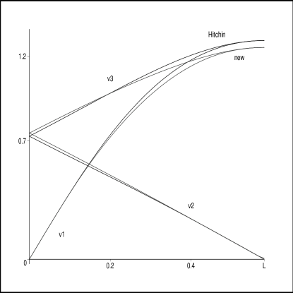
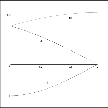
Figure 1. $v_{i}$ functions and Hitchin functions, as well as $h_{i}$.

5. Positivity of the determinants

As explained in Section 3, our proof will show that the modified curvature operator is positive definite by choosing the 4-form as in (3), with Püttmann parameters (3). For this we need to prove that the determinants of the $k\times k$ minors in the upper block of the $5\times 5$ matrices $A_{ij}$ (consisting of rows and columns 1 through $k$) are positive for $k=1,\dots,5$. We divide the interval $[0,L]$ into the three subintervals $[0,\frac{1}{10}],\ [\frac{1}{10},\frac{1}{2}]$ and $[\frac{1}{2},\frac{58}{100}]$ on which our metric is defined by polynomials. Each determinant is thus a rational function in the arclength parameter $t$ whose coefficients are rational as well. To show that it is positive, we use a theorem due to Sturm (see [Ja]) that gives a simple procedure for counting zeroes of a polynomial with rational coefficients on a closed interval in terms of a Euclidean algorithm.

To be specific, let $p(t)$ be a polynomial with integer coefficients. One inductively defines a finite sequence of polynomials (Sturm’s sequence) with $p_{1}=p(t)$, $p_{2}=p^{\prime}(t)$ and $p_{i+1}=-rem(p_{i},p_{i-1})$ where $rem()$ is the remainder of the polynomial division. If $p(t)$ and $p^{\prime}(t)$ have no common zeros, the last remainder $p_{k}(t)$ is a nonzero constant. Otherwise $p_{k}(t)=0$ and $p_{k-1}(t)$ is a common factor of $p(t)$ and $p^{\prime}(t)$, corresponding to double roots of $p(t)$, and thus $p$ and $p/p_{k-1}$ have the same zeroes. In this case the Sturm sequence for $p$ is that of $p/p_{k-1}$. Now Sturm’s theorem states that if $p_{i}(t),\ i=1\dots k$ is the Sturm sequence of $p(t)$, then the number of real zeroes in the half open interval $(a,b]$ is equal to the difference in the number of sign changes (not counting any zeroes) in the sequence $[p_{1}(a),\dots,p_{k}(a)]$ and the sequence $[p_{1}(b),\dots,p_{k}(b)]$. Since the endpoints of the 3 intervals are rational numbers, the same is true for the sequences $[p_{1}(a),\ldots,p_{k}(a)]$ and $[p_{1}(b),\ldots,p_{k}(b)]$. Thus the proof only deals with calculations involving rational numbers.

The degrees of the determinant polynomials are quite large, but one can easily modify the above procedure to significantly reduce these degrees, so that the proof can be carried out by hand: In each subinterval we translate the parameter $t$ in $v_{i}$ and $h_{i}$ so that the determinants are polynomials $f(s)$ of a variable $s$ defined in $[0,S]$. We define a new polynomial $g(s)$ that collects all the monomials in $f(s)$ with negative coefficient. Then the derivatives $g^{(k)}(s)$ are non-positive decreasing functions of $s$ for any $k\geq 0$. In particular $g^{(k)}(s)\geq g^{(k)}(S)$. If $f_{k}(s)$ denotes the truncated polynomial collecting the monomials of $f(s)$ of order $\leq k-1$, the remainder at a point $s\in[0,S]$ is given by Taylor’s formula and can be estimated by

$$\frac{1}{k!}f^{(k)}(s_{0}(s))s^{k}\geq\frac{1}{k!}g^{(k)}(s_{0}(s))s^{k}\geq\frac{1}{k!}g^{(k)}(S)S^{k}=R$$

independently of $s$. Since we choose $S$ to be rational, $R$ is rational as well. Then

$$f(s)\geq f_{k}(s)+R$$

and we prove that this last polynomial is positive in $[0,S]$ using Sturm’s theorem as above. In this procedure we need to divide the interval in the middle into 4 further subintervals. It turns out that the degree of $f_{k}$ will be smaller than $20$, in most cases smaller than $10$. A Maple program that carries out these calculations is made available at www.math.upenn.edu/~wziller/research.html. Notice that Maple can do this symbolically, i.e., no floating point operations are used.

For illustrative purposes, we draw the graph of the determinants in Figure 3. The determinants of the $4\times 4$ and $5\times 5$ minor in the matrix $A_{23}$ is not included in the second picture since its values lie between 5 and 25.

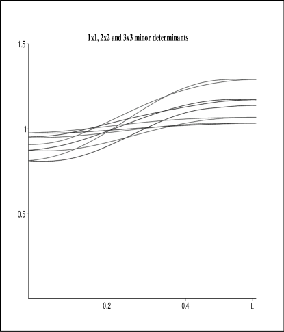
Figure 2. Determinants of all 5 minors in $A_{ij}$

6. Appendix

Smoothness of metrics on $P_{k}$ and $Q_{k}$.

At the endpoints $t=0$ and $t=L$, the principal orbits collapse and hence the functions need to satisfy certain smoothness conditions. Smoothness conditions for cohomogeneity one manifolds have been discussed, e.g., in [BH] and [EW]. For convenience of the reader, we present here an elementary proof in the case of codimension 2 orbits.

We do this first for arbitrary slopes $(p,q)$ of the circle $K_{\scriptscriptstyle{0}}\subset\operatorname{S}^{3}\times\operatorname{S}^{3}$ since this makes the discussion more transparent and for convenience we assume the singular orbit occurs at $t=0$. We will also assume that only the inner products in (1.2) are non-zero, although in this generality this is not necessarily true for all $G$ invariant metrics.

Theorem 6.1.

Let $H\subset K=\{e^{ip\theta},e^{iq\theta}\}\cdot H\subset G=\operatorname{S}^{3}\times\operatorname{S}^{3}$ be a singular orbit at $t=0$ with $H$ finite, $|H\cap K_{\scriptscriptstyle{0}}|=k$, and $\gcd(p,q)=1$. Assuming that $f_{i},g_{i},h_{i}$ are the only non-vanishing inner products, the metric is smooth if and only if:

• For the collapsing functions $f_{1},g_{1},h_{1}$ we have:

  $$f_{1},g_{1},h_{1}\text{ are even at }t =0\text{ and }$$

  $$p\;f_{1}=-q\;h_{1}\quad,\quad q\;g_{1} =-p\;h_{1}$$

  $$p^{2}\,f_{1}^{\prime\prime}+q^{2}\,g_{1}^{\prime\prime}+2pq\,h_{1}^{\prime\prime} =2k^{2}$$

• For the remaining functions we have:

  $$f_{2}+f_{3} =\phi_{3}(t^{2}) f_{2}-f_{3} =t^{\frac{4|p|}{k}}\phi_{4}(t^{2}),$$

  $$g_{2}+g_{3} =\phi_{5}(t^{2}) g_{2}-g_{3} =t^{\frac{4|q|}{k}}\phi_{6}(t^{2}),$$

  $$h_{2}+h_{3} =t^{\frac{2|q-p|}{k}}\phi_{7}(t^{2}) h_{2}-h_{3} =t^{\frac{2|q+p|}{k}}\phi_{8}(t^{2}).$$

  ’

where $\phi_{i}$ are smooth functions. When the exponent in $t$ is a fraction, the right hand side should be set to $0$.

Proof.

First notice that by $G$ invariance of the metric, it is smooth as long as the restriction to a slice $V$, i.e. a disc orthogonal to the singular orbit $G/K$, is smooth. The metric is defined along a line in $V$ and needs to be extended by $K_{\scriptscriptstyle{0}}$ invariance. Thus the issue is wether this extension is smooth at $0\in V$.

In the following sequence of lemmas we do not yet make any assumption on the group $G$, but only assume that the singular orbit $G/K$ has codimension 2. We start with the metric on the slice $V\simeq{\mathbb{R}}^{2}\simeq{\mathbb{C}}^{2}$. If $K_{\scriptscriptstyle{0}}=\{e^{i\theta}\mid 0\leq\theta\leq 2\pi\}$, the action on the slice is given by multiplication with $e^{ik\theta}$ since $|H\cap K^{0}|=k$. If we let $Z=\frac{d}{d\theta}\in{\mathfrak{k}}$ and $f(t)=|Z^{*}(c(t))|^{2}$, the usual proof for the smoothness of a metric in polar coordinates shows that

Lemma 6.2.

With the notation defined above, the metric on $V$ is smooth if and only if $f(t)=k^{2}t^{2}+t^{4}\phi(t^{2})$ for some smooth function $\phi$.

Let ${\mathfrak{g}}={\mathfrak{m}}\oplus{\mathfrak{k}}$ and ${\mathfrak{k}}={\mathfrak{h}}\oplus{\mathfrak{p}}$ be $Q$ orthogonal decompositions. Notice that $\dim{\mathfrak{p}}=1$ since $K/H$ is one dimensional. Furthermore, since $K_{\scriptscriptstyle{0}}=\operatorname{S}^{1}$, the $K_{\scriptscriptstyle{0}}$ irreducible modules in ${\mathfrak{m}}$ are either trivial or two dimensional. In the case of a trivial module we have:

Lemma 6.3.

Let $X$ be a vector in a one dimensional subspace ${\mathfrak{m}}_{0}$ of ${\mathfrak{m}}$ on which $K_{\scriptscriptstyle{0}}$ acts trivially, and $Z\in{\mathfrak{p}}$ as above. If the representation of $H$ on ${\mathfrak{m}}_{0}$ and ${\mathfrak{p}}$ are equivalent, then the metric is smooth if and only if, in addition to $f(t)=|Z^{*}|_{c(t)}^{2}=k^{2}t^{2}+t^{4}\phi_{1}(t^{2})$, we have

$$|X^{*}|_{c(t)}^{2}=\phi_{2}(t^{2}),\;\text{ and }\langle Z^{*},X^{*}\rangle_{c(t)}=t^{2}\phi_{3}(t^{2})$$

for some smooth functions $\phi_{i}$. If the representation of $H$ on ${\mathfrak{m}}_{0}$ and ${\mathfrak{p}}$ are inequivalent, we have $\langle Z^{*},X^{*}\rangle_{c(t)}=0$.

Indeed, since $K_{\scriptscriptstyle{0}}$ fixes $X$, the inner products are even functions of $t$. Furthermore, $Z^{*}$ and $X^{*}$ are orthogonal at $c(0)$ since the slice $V$ is orthogonal to the singular orbit $G/K$. The proof now is similar to the proof of Lemma 6.2.

If ${\mathfrak{m}}_{1}\subset{\mathfrak{m}}$ is a 2-dimensional $K_{\scriptscriptstyle{0}}$ irreducible module, invariant under $H$, we identify ${\mathfrak{m}}_{1}\simeq{\mathbb{C}}$, in which case the action of $K_{\scriptscriptstyle{0}}$ will be given by $z\to e^{id\theta}z$ for some $d\in{\mathbb{Z}}$. By possibly changing the order of the basis in ${\mathfrak{m}}_{1}$ and ${\mathfrak{p}}$ if necessary, we may assume that $d>0,k>0$. In the natural basis of ${\mathbb{C}}$ we let $g_{11},g_{22},g_{12}$ be the inner products of the basis vectors along $c(t)$.

Lemma 6.4.

With the notation defined above, the restriction of the metric to the $K$ irreducible module ${\mathfrak{m}}_{1}$ admits a smooth extension to the singular orbit if and only if $k$ divides $2d$ and

$$(g_{11}-g_{22})(t)=t^{2\frac{d}{k}}\phi_{1}(t^{2}),\qquad g_{12}(t)=t^{2\frac{d}{k}}\phi_{2}(t^{2}),\qquad(g_{11}+g_{22})(t)=\phi_{3}(t^{2})$$

where $\phi_{i}(t)$ are smooth functions. When the exponent in $t$ is a fraction, the right hand side should be set to $0$.

Proof.

We extend the inner products $g_{ij}$ to functions along the slice $V$. Let $P$ be the restriction of the metric tensor to ${\mathfrak{m}}_{1}$ and $R(\theta)$ represent a rotation by $\theta$. Since $e^{i\theta}\in K_{\scriptscriptstyle{0}}$ acts by $e^{ik\theta}$ on the slice $V\simeq{\mathbb{C}}$ and by $e^{id\theta}$ on ${\mathfrak{m}}_{1}$, the $K_{\scriptscriptstyle{0}}$ invariance of the metric can be written in matrix form:

$$P(e^{ik\theta}p)=R(d\theta)P(p)R(-d\theta),\;p\in V$$

In other words,

$$\left\{\begin{array}[]{l}g_{11}(e^{ik\theta}p)=\cos^{2}(d\theta)\,g_{11}(p)+\sin^{2}(d\theta)\,g_{22}(p)-2\sin(d\theta)\cos(d\theta)\,g_{12}(p)\\ g_{12}(e^{ik\theta}p)=(\cos^{2}(d\theta)-\sin^{2}(d\theta))\,g_{12}(p)-\sin(d\theta)\cos(d\theta)\,(g_{22}(p)-g_{11}(p))\\ g_{22}(e^{ik\theta}p)=\sin^{2}(d\theta)\,g_{11}(p)+\cos^{2}(d\theta)\,g_{22}(p)+2\sin(d\theta)\cos(d\theta)\,g_{12}(p)\\ \end{array}\right.$$

If we set $w=(g_{11}-g_{22})+2ig_{12}$, then one easily shows that the above equations are equivalent to:

$$\left\{\begin{array}[]{l}(g_{11}+g_{22})(e^{ki\theta}p)=(g_{11}+g_{22})(p))\\ w(e^{ki\theta}p)=e^{2di\theta}w(p)\end{array}\right.$$

Notice that if $w$ vanishes identically, this implies that the metric is smooth if and only if $g_{11}=g_{22}$ is even. If not, the second equation shows that $w$ is only well defined when $k$ divides $2d$. It then reduces to

$$w(te^{i\theta})=e^{2\frac{d}{k}i\theta}w(t),\ t\in{\mathbb{R}}$$

or equivalently

$$z^{-2\frac{d}{k}}w(z)=t^{-2\frac{d}{k}}w(t).$$

If $g(z)=z^{-2\frac{d}{k}}w(z)$, it follows that $g(z)$ and $g_{11}+g_{22}$ are $K$-invariant functions on $V$. Such functions admit a smooth extension to the origin if and only if they are even and thus

$$w(z)=z^{2\frac{d}{k}}(\phi_{1}({t}^{2})+i\phi_{2}({t}^{2})),\qquad(g_{11}+g_{22})(z)=\phi_{3}({t}^{2})$$

Separating the real and the imaginary part and restricting to the normal geodesic proves our claim. ∎

Next we deal with the case of two irreducible modules ${\mathfrak{m}}_{1}\simeq{\mathbb{C}}$ and ${\mathfrak{m}}_{2}\simeq{\mathbb{C}}$ under the action of $K_{\scriptscriptstyle{0}}$, whose restriction to $H$ are equivalent. Inner products between vectors in ${\mathfrak{m}}_{1}$ and ${\mathfrak{m}}_{2}$ are thus not necessarily 0. We choose bases $\{v_{1},w_{1}\}$ of ${\mathfrak{m}}_{1}$ and $\{v_{2},w_{2}\}$ of ${\mathfrak{m}}_{2}$ such that the action of $K_{\scriptscriptstyle{0}}$ on ${\mathfrak{m}}_{1}$ is given by $z\to e^{id\theta}z$ and on ${\mathfrak{m}}_{2}$ by $z\to e^{id^{\prime}\theta}z$ for some $d,d^{\prime}\in{\mathbb{Z}}$, and we can again assume that $d,d^{\prime},k$ are all positive. The inner products between ${\mathfrak{m}}_{1}$ and ${\mathfrak{m}}_{2}$ are then determined by $h_{11}=g(v_{1},v_{2})$, $h_{12}=g(v_{1},w_{2})$, $h_{21}=g(w_{1},v_{2})$ and $h_{22}=g(w_{1},w_{2})$ along $c(t)$. As in the proof of Lemma 6.4, one easily shows:

Lemma 6.5.

With the notation as above, the scalar products between elements of ${\mathfrak{m}}_{1}$ and ${\mathfrak{m}}_{2}$ admit a smooth extension to the singular orbit if and only if $k$ divides $d\pm d^{\prime}$ and

$$(h_{11}+h_{22})(t)=t^{\frac{d^{\prime}-d}{k}}\phi_{1}(t^{2}),\qquad(h_{11}-h_{22})(t)=t^{\frac{d^{\prime}+d}{k}}\phi_{2}(t^{2})$$

$$(h_{12}-h_{21})(t)=t^{\frac{d^{\prime}-d}{k}}\phi_{3}(t^{2}),\qquad(h_{12}+h_{21})(t)=t^{\frac{d^{\prime}+d}{k}}\phi_{4}(t^{2})$$

where $\phi_{i}(t),i=1,\ldots,4$, are smooth real functions. When the exponent in $t$ is a fraction, the right hand side should be set to $0$.

This sequence of lemmas deals with the general situation of a singular orbit of codimension 2. We now specialize to our situation with $G=\operatorname{S}^{3}\times\operatorname{S}^{3}$. Here we have, in terms of the basis $X_{i},Y_{i}$ of ${\mathfrak{g}}$, irreducible modules ${\mathfrak{m}}_{1}=\{X_{2},X_{3}\}$ and ${\mathfrak{m}}_{2}=\{Y_{2},Y_{3}\}$, a trivial module ${\mathfrak{m}}_{0}$ spanned by $W=-qX_{1}+pY_{1}$ and ${\mathfrak{p}}={\mathfrak{k}}$ spanned by $Z=pX_{1}+qY_{1}$.

Applying Lemma 6.2 and Lemma 6.3 (notice that $H$ acts the same on ${\mathfrak{p}}$ and ${\mathfrak{m}}_{0}$) we get:

$$|Z^{*}|^{2} =p^{2}\,f_{1}+q^{2}\,g_{1}+2pq\,h_{1}=k^{2}t^{2}+t^{4}\,\phi_{1}(t^{2})$$

$$\langle Z^{*},W^{*}\rangle =-pq\,f_{1}+pq\,g_{1}+(p^{2}-q^{2})\,h_{1}=t^{2}\phi_{2}(t^{2})$$

$$|W^{*}|^{2} =q^{2}\,f_{1}+p^{2}\,g_{1}-2pq\,h_{1}=\phi_{3}(t^{2})$$

This says in particular that $f_{1},g_{1},h_{1}$ must be even. The equations for the values of the functions and their first and second derivative at $t=0$ can be solved and give rise to the conditions in Theorem 6.1 (a).

On ${\mathfrak{m}}_{1}$ the isotropy group $K_{\scriptscriptstyle{0}}$ acts by rotation $R(2p\theta)$ and on ${\mathfrak{m}}_{2}$ by $R(2q\theta)$. Furthermore, the modules ${\mathfrak{m}}_{1}$ and ${\mathfrak{m}}_{2}$ are equivalent to each other under the action of $H$. Theorem 6.1 (b) then follows by applying Lemma 6.4 and Lemma 6.5. Notice that in our situation $g_{12}=h_{12}=h_{21}=0$, as required by $H$ invariance of the metric. This finishes the Proof of Theorem 6.1. ∎

Curvature tensor of metrics on $P_{k}$ and $Q_{k}$

The following gives the formula for the curvature tensor of a general cohomogeneity one metric on $P_{k}$ or $Q_{k}$ (and $R$).

Theorem 6.6.

A cohomogeneity one metric defined by $(f_{i},g_{i},h_{i})$ with $D_{i}=f_{i}g_{i}-h_{i}^{2}$, has the following components of the curvature tensor, all others being $0$.

$$R_{X_{i}Y_{i}X_{i}Y_{i}}= -\frac{1}{4}(f_{i}^{\prime}g_{i}^{\prime}-{h_{i}^{\prime}}^{2}).$$

$$R_{X_{i}Y_{i}X_{j}Y_{j}}= -h_{k}-\frac{1}{D_{k}}\left\{h_{i}h_{j}(f_{k}+g_{k})+h_{k}(f_{i}g_{j}+f_{j}g_{i})-h_{k}(D_{i}+D_{j})\right\}.$$

$$R_{X_{i}X_{j}X_{i}X_{j}}= 2f_{i}+2f_{j}-3f_{k}-\frac{1}{4}f_{i}^{\prime}f_{j}^{\prime}+\frac{1}{D_{k}}g_{k}(f_{i}-f_{j})^{2}.$$

$$R_{X_{i}X_{j}X_{i}Y_{j}}= h_{j}-\frac{1}{4}f_{i}^{\prime}h_{j}^{\prime}-\frac{1}{D_{k}}(f_{i}-f_{j})(h_{j}g_{k}+h_{i}h_{k}).$$

$$R_{X_{i}X_{j}Y_{i}Y_{j}}= -2h_{k}-\frac{1}{4}h_{i}^{\prime}h_{j}^{\prime}-\frac{1}{D_{k}}\left\{h_{i}h_{j}(f_{k}+g_{k})+h_{k}(h_{i}^{2}+h_{j}^{2})\right\}.$$

$$R_{X_{i}Y_{j}X_{i}Y_{j}}= -\frac{1}{4}f_{i}^{\prime}g_{j}^{\prime}+\frac{1}{D_{k}}\left\{h_{i}^{2}f_{k}+h_{j}^{2}g_{k}+2h_{i}h_{j}h_{k}\right\}.$$

$$R_{X_{i}Y_{j}X_{j}Y_{i}}= h_{k}+\frac{1}{4}h_{i}^{\prime}h_{j}^{\prime}+\frac{1}{D_{k}}h_{k}(f_{i}-f_{j})(g_{i}-g_{j}).$$

$$R_{Y_{i}Y_{j}X_{i}Y_{j}}= h_{i}-\frac{1}{4}h_{i}^{\prime}g_{j}^{\prime}+\frac{1}{D_{k}}(h_{j}h_{k}+h_{i}f_{k})(g_{i}-g_{j}).$$

$$R_{Y_{i}Y_{j}Y_{i}Y_{j}}= 2g_{i}+2g_{j}-3g_{k}-\frac{1}{4}g_{i}^{\prime}g_{j}^{\prime}+\frac{1}{D_{k}}f_{k}(g_{i}-g_{j})^{2}.$$

$$R_{X_{i}X_{j}X_{k}T}= \frac{1}{2}f_{i}^{\prime}+\frac{1}{2}f_{j}^{\prime}-f_{k}^{\prime}+\frac{1}{2D_{i}}(f_{j}-f_{k})(g_{i}f_{i}^{\prime}-h_{i}h_{i}^{\prime})-\frac{1}{2D_{j}}(f_{i}-f_{k})(g_{j}f_{j}^{\prime}-h_{j}h_{j}^{\prime}).$$

$$R_{X_{i}X_{j}Y_{k}T}= -h_{k}^{\prime}+\frac{1}{2D_{i}}\left\{h_{j}(f_{i}h_{i}^{\prime}-h_{i}f_{i}^{\prime})-h_{k}(g_{i}f_{i}^{\prime}-h_{i}h_{i}^{\prime})\right\}$$

$$\hskip 150.0pt-\frac{1}{2D_{j}}\left\{h_{i}(f_{j}h_{j}^{\prime}-h_{j}f_{j}^{\prime})-h_{k}(g_{j}f_{j}^{\prime}-h_{j}h_{j}^{\prime})\right\}.$$

$$R_{X_{i}Y_{j}X_{k}T}= \frac{1}{2}h_{j}^{\prime}+\frac{1}{2D_{i}}\left\{h_{j}(g_{i}f_{i}^{\prime}-h_{i}h_{i}^{\prime})-h_{k}(f_{i}h_{i}^{\prime}-h_{i}f_{i}^{\prime})\right\}-\frac{1}{2D_{j}}(f_{i}-f_{k})(g_{j}h_{j}^{\prime}-h_{j}g_{j}^{\prime})$$

$$R_{X_{i}Y_{j}Y_{k}T}= \frac{1}{2}h_{i}^{\prime}+\frac{1}{2D_{i}}(g_{j}-g_{k})(f_{i}h_{i}^{\prime}-h_{i}f_{i}^{\prime})-\frac{1}{2D_{j}}\left\{h_{i}(f_{j}g_{j}^{\prime}-h_{j}h_{j}^{\prime})-h_{k}(g_{j}h_{j}^{\prime}-h_{j}g_{j}^{\prime})\right\}$$

$$R_{Y_{i}Y_{j}X_{k}T}= -h_{k}^{\prime}+\frac{1}{2D_{i}}\left\{h_{j}(g_{i}h_{i}^{\prime}-h_{i}g_{i}^{\prime})-h_{k}(f_{i}g_{i}^{\prime}-h_{i}h_{i}^{\prime})\right\}$$

$$\hskip 150.0pt-\frac{1}{2D_{j}}\left\{h_{i}(g_{j}h_{j}^{\prime}-h_{j}g_{j}^{\prime})-h_{k}(f_{j}g_{j}^{\prime}-h_{j}h_{j}^{\prime})\right\}.$$

$$R_{Y_{i}Y_{j}Y_{k}T}= \frac{1}{2}g_{i}^{\prime}+\frac{1}{2}g_{j}^{\prime}-g_{k}^{\prime}+\frac{1}{2D_{i}}(g_{j}-g_{k})(f_{i}g_{i}^{\prime}-h_{i}h_{i}^{\prime})-\frac{1}{2D_{j}}(g_{i}-g_{k})(f_{j}g_{j}^{\prime}-h_{j}h_{j}^{\prime})$$

$$R_{X_{i}TX_{i}T}= -\frac{1}{2}f_{i}^{\prime\prime}+\frac{1}{4D_{i}}\left\{g_{i}{f_{i}^{\prime}}^{2}+f_{i}{h_{i}^{\prime}}^{2}-2h_{i}f_{i}^{\prime}h_{i}^{\prime}\right\}.$$

$$R_{X_{i}TY_{i}T}= -\frac{1}{2}h_{i}^{\prime\prime}+\frac{1}{4D_{i}}\left\{g_{i}f_{i}^{\prime}h_{i}^{\prime}+f_{i}h_{i}^{\prime}g_{i}^{\prime}-h_{i}f_{i}^{\prime}g_{i}^{\prime}-h_{i}{h_{i}^{\prime}}^{2}\right\}.$$

$$R_{Y_{i}TY_{i}T}= -\frac{1}{2}g_{i}^{\prime\prime}+\frac{1}{4D_{i}}\left\{g_{i}{h_{i}^{\prime}}^{2}+f_{i}{g_{i}^{\prime}}^{2}-2h_{i}h_{i}^{\prime}g_{i}^{\prime}\right\}.$$

with $(i,j,k)$ is a cyclic permutation of $(1,2,3)$.

Proof.

We will use the following curvature formulas for a cohomogeneity one metric (see [GZ2]):

$$g(R(X,Y)Z,W)= -\tfrac{1}{2}Q(B_{-}(X,Y),[Z,W])-\tfrac{1}{2}Q([X,Y],B_{-}(Z,W))$$

$$+\tfrac{1}{2}Q(P[X,Y]_{{\mathfrak{n}}},[Z,W]_{{\mathfrak{n}}})+\tfrac{1}{4}Q(P[X,Z]_{{\mathfrak{n}}},[Y,W]_{{\mathfrak{n}}})$$

$$-\tfrac{1}{4}Q(P[X,W]_{{\mathfrak{n}}},[Y,Z]_{{\mathfrak{n}}})$$

$$+Q(B_{+}(X,Z),P^{-1}B_{+}(Y,W))-Q(B_{+}(X,W),P^{-1}B_{+}(Y,Z))$$

$$+\tfrac{1}{4}Q(P^{\prime}X,Z)Q(P^{\prime}Y,W)-\tfrac{1}{4}Q(P^{\prime}X,W)Q(P^{\prime}Y,Z)$$

$$g(R(X,Y)Z,T)=\> \tfrac{1}{2}Q([X,Y],P^{\prime}Z)-\tfrac{1}{4}Q([Z,X],P^{\prime}Y)-\tfrac{1}{4}Q([Y,Z],P^{\prime}X)$$

$$-\tfrac{1}{2}Q(P^{\prime}X,P^{-1}B_{+}(Y,Z))+\tfrac{1}{2}Q(P^{\prime}Y,P^{-1}B_{+}(Z,X))$$

$$g(R(X,T)T,Y)=\> Q((-\tfrac{1}{2}P^{\prime\prime}+\tfrac{1}{4}P^{\prime}P^{-1}P^{\prime})X,Y)$$

where $P$ defines the metric via $g(X^{*},Y^{*})=Q(P(X),Y)$ and $B_{\pm}(X,Y)=\frac{1}{2}([X,PY]\mp[PX,Y])$.

For our metrics we have

$$PX_{i}=f_{i}X_{i}+h_{i}Y_{i}\ ,\ PY_{i}=h_{i}X_{i}+g_{i}Y_{i}$$

and thus

$$P^{-1}X_{i}=\frac{1}{D_{i}}(g_{i}X_{i}-h_{i}Y_{i})\ ,\ P^{-1}Y_{i}=\frac{1}{D_{i}}(-h_{i}X_{i}+fY_{i})$$

Since $[X_{i},X_{j}]=2X_{k}\ ,\ [Y_{i},Y_{j}]=2Y_{k}$, one has

$$B_{\pm}(X_{i},X_{i}) =B_{\pm}(Y_{i},Y_{i})=B_{\pm}(X_{i},Y_{i})=0$$

$$B_{\pm}(X_{i},X_{j}) =(f_{j}\mp f_{i})X_{k}\ ,\ B_{\pm}(Y_{i},Y_{j})=(g_{j}\mp g_{i})Y_{k}\ ,\ B_{\pm}(X_{i},Y_{j})=(h_{j}X_{k}\mp h_{i}Y_{k})$$

with $(i,j,k)$ cyclic. The formulas for the curvature tensor now easily follow by substituting. ∎

Using these formulas, one also easily derives the curvature formulas for a connection metric in Theorem 2.7. We illustrate the procedure in one particular case, the others being similar.

Proof of Theorem 2.7:  We will show that $\langle R(X_{i}^{*},\bar{Z}_{j})\bar{Z}_{k},T\rangle=\epsilon B_{ij}$.

Notice that since $V_{i}=Y_{i}^{*}-h_{i}X_{i}^{*}=v_{i}\bar{Z}_{i}$ are not action fields, [GZ2] can not be applied directly. By expansion, we have:

$$v_{j}v_{k} \langle R(X_{i}^{*},\bar{Z}_{j})\bar{Z}_{k},T\rangle=\langle R(X_{i}^{*},V_{j})V_{k},T\rangle=\langle R(X_{i}^{*},Y_{j}^{*}-h_{j}X_{j}^{*})(Y_{k}^{*}-h_{k}X_{k}^{*}),T\rangle$$

$$=\langle R(X_{i}^{*},Y_{j}^{*})Y_{k}^{*},T\rangle-h_{j}\langle R(X_{i}^{*},X_{j}^{*})Y_{k}^{*},T\rangle-h_{k}\langle R(X_{i}^{*},Y_{j}^{*})X_{k}^{*}),T\rangle$$

$$\quad+h_{j}h_{k}\langle R(X_{i}^{*},X_{j}^{*})X_{k}^{*},T\rangle$$

We now use the curvature formulas from Theorem 6.6, where we replace $f_{i}$ by $\epsilon$, $h_{i}$ by $\epsilon h_{i}$ and $g_{i}$ by $v_{i}^{2}+\epsilon h_{i}^{2}$, as discussed in (2.2) for a scaled connection metric. We thus have

$$\langle R(X_{i}^{*},Y_{j}^{*})Y_{k}^{*},T\rangle=\frac{\epsilon}{2}\left(\frac{v_{i}^{2}+v_{k}^{2}-v_{j}^{2}}{v_{i}^{2}}h_{i}^{\prime}+h_{k}h_{j}^{\prime}-2(h_{i}+h_{j}h_{k})\frac{v_{j}^{\prime}}{v_{j}}\right)$$

$$\hskip 100.0pt+\frac{\epsilon^{2}}{2}\left(\frac{(h_{k}^{2}-h_{j}^{2})h_{i}^{\prime}}{v_{i}^{2}}-\frac{h_{j}h_{j}^{\prime}(h_{i}+h_{j}h_{k})}{v_{j}^{2}}\right)$$

$$\langle R(X_{i}^{*},X_{j}^{*})Y_{k}^{*},T\rangle=-\epsilon h_{k}^{\prime}-\frac{\epsilon^{2}}{2}\left(\frac{h_{i}^{\prime}}{v_{i}^{2}}(h_{j}+h_{i}h_{k})+\frac{h_{j}^{\prime}}{v_{j}^{2}}(h_{i}+h_{j}h_{k})\right)$$

$$\langle R(X_{i}^{*},Y_{j}^{*})X_{k}^{*},T\rangle=\epsilon\frac{h_{j}^{\prime}}{2}+\frac{\epsilon^{2}}{2}\frac{h_{i}^{\prime}}{v_{i}^{2}}(h_{k}+h_{i}h_{j})$$

$$\langle R(X_{i}^{*},X_{j}^{*})X_{k}^{*},T\rangle=0$$

Combining these:

$$v_{j}v_{k}\langle R(X_{i}^{*},\bar{Z}_{j})\bar{Z}_{k},T\rangle = \frac{\epsilon}{2}\left(\frac{v_{i}^{2}+v_{k}^{2}-v_{j}^{2}}{v_{i}^{2}}h_{i}^{\prime}+h_{k}h_{j}^{\prime}-2(h_{i}+h_{j}h_{k})\frac{v_{j}^{\prime}}{v_{j}}+2h_{j}h_{k}^{\prime}-h_{k}h_{j}^{\prime}\right)$$

$$+ \frac{\epsilon^{2}}{2}\left(\frac{(h_{k}^{2}-h_{j}^{2})h_{i}^{\prime}}{v_{i}^{2}}-\frac{h_{j}h_{j}^{\prime}(h_{i}+h_{j}h_{k})}{v_{j}^{2}}\right.$$

$$\hskip 15.0pt+\left.h_{j}\frac{h_{i}^{\prime}}{v_{i}^{2}}(h_{j}+h_{i}h_{k})+h_{j}\frac{h_{j}^{\prime}}{v_{j}^{2}}(h_{i}+h_{j}h_{k})-h_{k}\frac{h_{i}^{\prime}}{v_{i}^{2}}(h_{k}+h_{i}h_{j})\right)$$

and thus

$$v_{j}v_{k}\langle R(X_{i}^{*},\bar{Z}_{j})\bar{Z}_{k},T\rangle=\epsilon(h_{j}h_{k}^{\prime}+\frac{v_{k}^{2}+v_{i}^{2}-v_{j}^{2}}{2v_{i}^{2}}h_{i}^{\prime}-\frac{v_{j}^{\prime}}{v_{j}}(h_{i}+h_{j}h_{k}))=\epsilon v_{j}v_{k}B_{ij}$$

which shows that $\langle R(X_{i}^{*},\bar{Z}_{j})\bar{Z}_{k},T\rangle=\epsilon B_{ij}$.

We finally indicate how to prove the curvature formulas in (2) for the metric on the base. In this case the metric is diagonal $PW^{*}_{i}=v_{i}^{2}W^{*}_{i}$ and thus $B_{\pm}(W_{i},W_{i})=0$ and $B_{\pm}(W_{i},W_{j})=(v_{j}^{2}\mp v_{i}^{2})W_{k}$, from which (2) easily follows as in the proof of Theorem 6.6.

References

• [AA] A.V. Alekseevsy and D.V. Alekseevsy, $G$- manifolds with one dimensional orbit space, Ad. in Sov. Math. 8 (1992), 1–31.
• [AW] S. Aloff and N. Wallach, An infinite family of 7–manifolds admitting positively curved Riemannian structures, Bull. Amer. Math. Soc. 81(1975), 93–97.
• [BH] A. Back and W.Y. Hsiang, Equivariant geometry and Kervaire spheres, Trans. Amer. Math. Soc. 304 (1987), no. 1, 207–227.
• [Ba] Y.V. Bazaikin, On a certain family of closed 13–dimensional Riemannian manifolds of positive curvature, Sib. Math. J. 37, No. 6 (1996), 1219-1237.
• [BB] L. Bérard Bergery, Les variétés riemanniennes homogènes simplement connexes de dimension impaire à courbure strictement positive, J. Math. pure et appl. 55 (1976), 47–68.
• [Be] M. Berger, Les variétés riemanniennes homogenes normales simplement connexes a courbure strictment positive, Ann. Scuola Norm. Sup. Pisa 15 (1961), 191-240.
• [BW] C. Böhm, B. Wilking, Manifolds with positive curvature operators are space forms, Ann. of Math. 167 (2008), 1079–1097.
• [CDR] L.M Chaves, A.  Derdziński and A. Rigas, A condition for positivity of curvature, Bol. Soc. Brasil. Mat. (N.S.) 23 (1992), 153–165.
• [Cr] D. Crowley, The classification of highly connected manifolds in dimensions 7 and 15, Thesis, Indiana University, 2001 ,math.GT/0203253.
• [CE] D. Crowley and C. Escher, The classification of $\mathbb{S}^{3}$-bundles over $\mathbb{S}^{4}$, Diff. Geom. Appl. 18, (2003) 363-380.
• [DR] A. Derdzinski and A.  Rigas. Unflat connections in 3-sphere bundles over $\mathbb{S}^{4}$, Trans. of the AMS, 265 (1981), 485–493.
• [De1] O. Dearricott, Positive sectional curvature on 3-Sasakian manifolds, Ann. Global Anal. Geom. 25 (2004), 59–72.
• [De2] O. Dearricott, A 7-manifold with positive curvature, to appear in Duke Math. J.
• [E1] J.H. Eschenburg, New examples of manifolds with strictly positive curvature, Inv. Math 66 (1982), 469-480.
• [E2] J.H. Eschenburg, Freie isometrische Aktionen auf kompakten Lie-Gruppen mit positiv gekrümmten Orbiträumen, Schriftenr. Math. Inst. Univ. Münster 32 (1984).
• [EW] J.H. Eschenburg and M. Wang, The initial value problem for cohomogeneity one Einstein metrics, J. Geom. Anal. 10 (2000), 109–137.
• [FR] F. Fang and X. Rong, Positive pinching, volume and second Betti number, Geom. Funct. Anal. 9 (1999), 641–674.
• [FZ] L. Florit and W. Ziller, Orbifold fibrations of Eschenburg spaces, Geom. Ded. 127 (2007), 159–175.
• [G] S.  Goette, Adiabetic limits of Seifert fibrations, Dedekind sums and the diffeomrphism type of certain 7-manifolds, Preprint.
• [Gr] K. Grove, Geometry of, and via, Symmetries, Amer. Math. Soc. Univ. Lecture Series 27 (2002), 31–53.
• [GVZ] K. Grove, L. Verdiani and W. Ziller, A new type of a positively curved manifolds, Preprint 2008, arXiv;0809.2304.
• [GWZ] K. Grove, B. Wilking and W. Ziller, Positively curved cohomogeneity one manifolds and 3-Sasakian geometry, J. Diff. Geom. 78 (2008), 33–111.
• [GZ1] K. Grove and W. Ziller, Curvature and symmetry of Milnor spheres, Ann. of Math. 152 (2000), 331–367.
• [GZ2] K. Grove and W. Ziller, Cohomogeneity one manifolds with positive Ricci curvature, Inv. Math. 149 (2002), 619-646.
• [Hi1] N. Hitchin, A new family of Einstein metrics, Manifolds and geometry (Pisa, 1993), 190–222, Sympos. Math., XXXVI, Cambridge Univ. Press, Cambridge, 1996.
• [Hi2] N. Hitchin, Poncelet polygons and the Painlevé equations, Proc of TATA Institute Conference 1991.
• [Ja] N. Jacobson, Basic Algebra, Freeman & Co., 1974
• [KS] N. Kitchloo and K.Shankar, On Complexes Equivalent to $S^{3}$-bundles over $S^{4}$, Int. Math. Res. Notices, 8 (2001), 381 -394.
• [KZ] V. Kapovitch and W. Ziller, Biquotients with singly generated rational cohomology, Geom. Dedicata 104 (2004), 149-160.
• [Mü] P. Müter, Krümmungserhöhende Deformationen mittels Gruppenaktionen, Ph.D. thesis, Univerity of Münster, 1987.
• [PW1] P. Petersen and F. Wilhelm, Examples of Riemannian manifolds with positive curvature almost everywhere, Geom. Topol. 3 (1999), 331–367.
• [PW2] P. Petersen and F. Wilhelm, An exotic sphere with positive sectional curvature, preprint.
• [PT] A. Petrunin and W. Tuschmann, Diffeomorphism finiteness, positive pinching, and second homotopy, Geom. Funct. Anal. 9 (1999), 736–774.
• [Pü] T. Püttmann, Optimal pinching constants of odd-dimensional homogeneous spaces, Invent. Math. 138 (1999), 631–684.
• [Th1] J.A. Thorpe, On the curvature tensor of a positively curved $4$-manifold, Mathematical Congress, Dalhousie Univ., Halifax, N.S., Canad. Math. Congr., Montreal, Que. (1972), 156–159.
• [Th2] J.A. Thorpe, The zeros of nonnegative curvature operators, J. Diff. Geom., 5, (1971), 113–125. err., J. Diff. Geom. 11, (1976), 315.
• [To] B. Totaro, Cheeger Manifolds and the Classification of Biquotients, J. Diff. Geom. 61 (2002), 397 -451.
• [V1] L. Verdiani, Cohomogeneity one Riemannian manifolds of even dimension with strictly positive sectional curvature, I, Math. Z. 241 (2002), 329–339.
• [V2] L. Verdiani, Cohomogeneity one manifolds of even dimension with strictly positive sectional curvature, J. Diff. Geom. 68 (2004), 31–72.
• [VZ1] L. Verdiani and W. Ziller, Positively curved homogeneous metrics on spheres, Math. Zeitschrift, 261 (2009), 473–488.
• [VZ2] L. Verdiani and W. Ziller, Obstructions in positive curvature, preprint.
• [Wa] N. Wallach, Compact homogeneous Riemannian manifolds with strictly positive curvature, Ann. of Math. 96 (1972), 277-295.
• [Wi1] B. Wilking, The normal homogeneous space $(\operatorname{SU}(3)\times\operatorname{SO}(3))/\operatorname{U}(2)$ has positive sectional curvature, Proc. of Amer. Math. Soc. 127 (1999), 1191-1994.
• [Wi2] B. Wilking, Nonnegatively and Positively Curved Manifolds, Surveys in Differential Geometry, Vol. XI: Metric and Comparison Geometry, ed. J.Cheeger and K.Grove, International Press (2007).
• [Zi1] W. Ziller, Examples of manifolds with nonnegative sectional curvature, in: Metric and Comparison Geometry, ed. J.Cheeger and K.Grove, Surv. Diff. Geom. Vol. XI, International Press (2007).
• [Zi2] W. Ziller, Geometry of positively curved cohomogeneity one manifolds, in: Topology and Geometric Structures on Manifolds, in honor of Charles P.Boyer’s 65th birthday, Progress in Mathematics, Birkhäuser, (2008).
• [Zo] S. Zoltek, Nonnegative curvature operators: some nontrivial examples, J. Diff. Geom. 14 (1979), 303-315.