A simple toy model of the advective-acoustic instability. II. Numerical simulations

Abstract

The physical processes involved in the advective-acoustic instability are investigated with 2D numerical simulations. Simple toy models, developed in a companion paper, are used to describe the coupling between acoustic and entropy/vorticity waves, produced either by a stationary shock or by the deceleration of the flow. Using two Eulerian codes based on different second order upwind schemes, we confirm the results of the perturbative analysis. The numerical convergence with respect to the computation mesh size is studied with 1D simulations. We demonstrate that the numerical accuracy of the quantities that depend on the physics of the shock is limited to a linear convergence. We argue that this property is likely to be true for most current numerical schemes dealing with SASI in the core-collapse problem, and could be solved by the use of advanced techniques for the numerical treatment of the shock. We propose a strategy to choose the mesh size for an accurate treatment of the advective-acoustic coupling in future numerical simulations.

1. Introduction

Most of our knowledge about the possible consequences of SASI on the core-collapse problem has been built, over the last 5 years, on the results of multidimensional numerical simulations (e.g. Blondin et al., 2003; Scheck et al., 2004; Burrows et al., 2006; Blondin & Mezzacappa, 2007; Marek & Janka, 2007; Iwakami et al., 2008). Whether or not SASI can contribute to overcome the explosion threshold, to kick the neutron star and alter its spin is still debated. In addition to the fundamental uncertainties associated with the equation of state of dense matter or the numerical treatment of neutrino transport, some difficulties are simply related to multidimensional hydrodynamics (Blondin et al., 2003; Ohnishi et al., 2006; Blondin & Mezzacappa, 2006, 2007; Iwakami et al., 2008). This latter difficulty is partly due to the complexity of the mechanism underlying SASI, which is at best unfamiliar, and possibly also affected by the different numerical techniques used by different groups. The present study aims at improving our understanding of the instability mechanism at work by studying the advective-acoustic instability in the highly simplified set up introduced in the first paper of this series (Foglizzo, 2008,  hereafter paper I). We note that a debate exists about the nature of this mechanism, as witnessed by Blondin & Mezzacappa (2006,  hereafter BM06), Foglizzo et al. (2007,  hereafter FGS07), Laming (2007), Yamasaki & Foglizzo (2008) and Laming (2008). Thus we believe that a better understanding of the advective-acoustic instability in simple examples can help recognise it in more complex situations. The separation of the advective-acoustic cycle into two separate problems is necessary in order to identify, between advected and acoustic perturbations, the consequences of each one on the other, as seen on Fig. 7 of Blondin et al. (2003) or Figs. 11-12 of Scheck et al. (2008). In paper I, the following questions were answered through a perturbative analysis:

(i) what are the amplitudes of the entropy and vorticity waves generated by a shock perturbed by an acoustic wave propagating against the flow, towards the shock?

(ii) what is the amplitude of the acoustic wave generated by the deceleration of an entropy/vorticity wave through a localised gravitational potential?

The first purpose of our study is thus to check the results of the perturbative analysis presented in paper I through numerical experiments, thus providing concrete examples of the coupling processes involved.

The second purpose of this study is to gain confidence in the results of more elaborate numerical simulations by assessing their accuracy using our simple set up. The 2D numerical simulations of BM06 showed some globally good agreement with the perturbative analysis of FGSJ07. The typical error on the growth rate and the oscillation frequency of SASI, around $30\%$, was not small though. Could this be a concern for the many other simulations which use a coarser mesh size? We wish to evaluate quantitatively, using our simple toy model, to what extent the advective-acoustic instability can be affected by numerical resolution.

The paper is organised as follows. In Sect. 2, the set up of the simulations is described and the numerical codes are presented. Sect. 3 illustrates qualitatively the two coupling processes involved in the advective-acoustic instability using 2D simulations. A quantitative analysis of these simulations is also performed which validates both the perturbative analysis and the numerical technique. In Sect. 4, we evaluate the rate of numerical convergence with respect to the mesh size, using a series of 1D numerical simulations. While the accuracy of the acoustic feedback produced by the flow gradients is quadratic with respect to the mesh size, the accuracy of the entropy wave produced by the shock depends on the mesh size only linearly. The linear phase of the full problem is simulated in Sect. 5, where the oscillation frequency and growth rate are compared to the results of the perturbative analysis. The consequences of these numerical difficulties for the simulations of core-collapse supernovae are discussed in Sect. 6.

2. Numerical techniques and set up of the simulations

2.1. Numerical techniques

The governing equations are solved using the AUSMDV scheme (Wada & Liou, 1994), which is a second-order finite volume scheme. The former version of AUSMDV was called “advection upstream splitting method” (AUSM) and developed by Liou & Steffen (1993). AUSM is a remarkably simple upwind flux vector splitting scheme that treats the convective and pressure terms of the flux function separately. In the AUSMDV, a blending form of AUSM and flux difference is used, and the robustness of AUSM in dealing with strong shocks is improved. A great advantage of this scheme is the reduction of numerical viscosity, which gives sharp preservation of fluid interfaces and high resolution feature as in the “piecewise parabolic method” (PPM) of Colella & Woodward (1984). Some advantages over PPM are simplicity and a lower computational cost. In Sect. 4, the numerical results obtained with AUSMDV are compared with those computed using RAMSES (Teyssier, 2002). RAMSES is also a second order shock–capturing code. It uses the MUSCL–Hancok scheme to update the MHD equation. For the simulations presented in sect. 5, we used the MinMod slope limiter along with the HLLD Riemann solver (Miyoshi & Kusano, 2005), which reduces to the HLLC Riemann solver (Toro et al., 1994) in the hydrodynamic case dealt with in this paper.

2.2. General set up

Figure 1.— Schematic view of the advective-acoustic cycle occurring in the toy model, separated in two sub problems. Entropy/vorticity perturbations are noted as circular arrows, while acoustic waves are noted as wavy arrows. The linear coupling between waves is measured by the efficiencies ${\cal Q}_{\rm sh}$, ${\cal Q}_{\nabla}$, ${\cal R}_{\rm sh}$ and ${\cal R}_{\nabla}$.

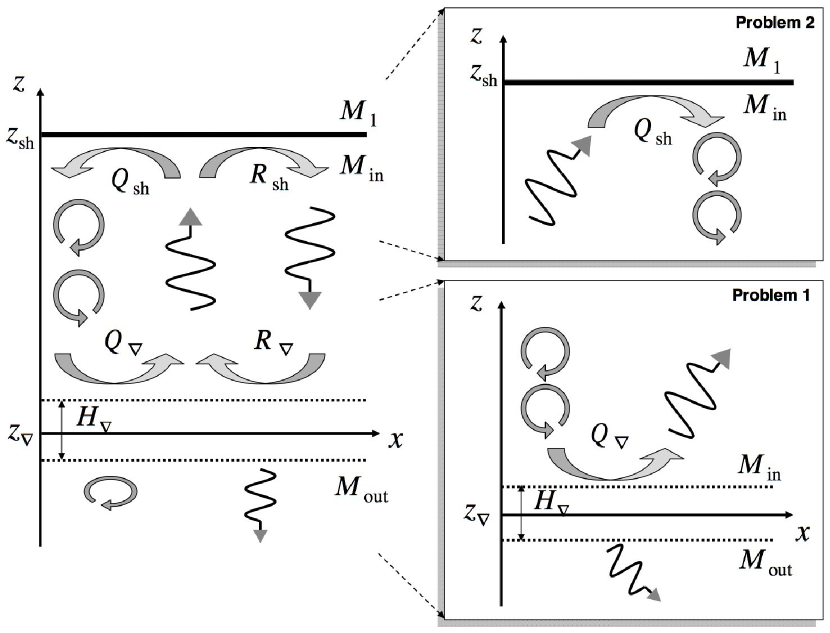
In this section, we describe the problems we designed to illustrate the physical mechanisms underlying the advective–acoustic instability. Our “Problem 1” is aimed at studying the interaction of waves in a stationary subsonic flow decelerated across a localised external potential, whereas “Problem 2” studies the interaction of waves with a stationary shock in a uniform potential. Both problems were described in detail in the linear approximation in paper I, and are schematically illustrated by Fig. 1. Let us recall that the stationary flow is uniform in the $x$ direction, and flows along the $z$ direction with a negative velocity. The ideal gas satisfies a polytropic equation of state with an adiabatic index $\gamma=4/3$, and a measure of the entropy is defined as $S\equiv(\log(p/\rho^{\gamma}))/(\gamma-1)$. The horizontal size of the computation domain is noted $L_{x}$. The index “1” refers to the supersonic flow ahead of the shock ($z>z_{\rm sh}$), and “in” refers to the subsonic region after the shock ($z<z_{\rm sh}$). ${\cal M}_{\rm in}$, $v_{1}$ and $\rho_{1}$ are determined by the Rankine-Hugoniot relations as follows:

$${\cal M}_{\rm in} = \left(\frac{2+\left(\gamma-1\right){\cal M}_{1}^{2}}{2\gamma{\cal M}_{1}^{2}-\gamma+1}\right)^{\frac{1}{2}},$$ (1)

$${v_{1}\over v_{\rm in}} = \frac{\left(\gamma+1\right){\cal M}_{1}^{2}}{2+\left(\gamma-1\right){\cal M}_{1}^{2}},$$ (2)

$${\rho_{1}\over\rho_{\rm in}} = \frac{v_{\rm in}}{v_{1}},$$ (3)

where $v_{\rm in}=-{\cal M}_{\rm in}c_{\rm in}$. The incident Mach number is chosen as ${\cal M}_{1}=5$. Thus ${\cal M}_{\rm in}\sim 0.39$.

A region of deceleration extends over a width $\sim H_{\nabla}$ centred on $z_{\nabla}=0$, separating two uniform subsonic regions indexed by “in” and “out”, respectively. The external potential $\Delta\Phi(z)$ responsible for the flow gradients is defined by

$$\Phi(z)\equiv\frac{\Delta\Phi}{2}\left[\tanh\left(\frac{z-z_{\nabla}}{H_{\nabla}/2}\right)+1\right].$$ (4)

The potential jump $\Delta\Phi>0$ is set by specifying the sound speed ratio $c_{\rm{in}}/c_{\rm{out}}$:

$$\Delta\Phi=\left(\frac{{\cal M}_{\rm out}^{2}}{2}+\frac{1}{\gamma-1}\right)c_{\rm out}^{2}-\left(\frac{{\cal M}_{\rm in}^{2}}{2}+\frac{1}{\gamma-1}\right)c_{\rm in}^{2}.$$ (5)

Defining $H\equiv z_{\rm sh}-z_{\nabla}$, we adopt $H_{\nabla}/H=0.1$ and $c_{\rm in}^{2}/c_{\rm out}^{2}=0.75$ in this study, as in paper I.

Time is normalised by $\tau_{\rm aac}$, which is a reference timescale associated to the advective-acoustic cycle defined as follow:

$$\tau_{\rm aac}\equiv{1\over 1-{\cal M}_{\rm in}}\;\;{H\over|v_{\rm in}|}.$$ (6)

The advection time through the deceleration region $\tau_{\nabla}$ is associated in paper I to a frequency cut-off $\omega_{\nabla}$, above which the efficiency of acoustic feedback decreases:

$$\tau_{\nabla} \equiv \int_{z_{\rm\nabla}-H_{\nabla}/2}^{z_{\rm\nabla}+H_{\nabla}/2}{{\rm d}r\over|v|},$$ (7)

$$\omega_{\nabla} \sim {1\over\tau_{\nabla}}.$$ (8)

Units are chosen such that $c_{\rm in}=1$, $\rho_{\rm in}=1$ and $H=1$. Since $p=\rho c^{2}/\gamma$ and $\gamma=4/3$, then $p_{\rm in}=0.75$ and $S_{\rm in}\sim-0.86$. The reference timescale is thus $\tau_{\rm aac}\sim 4.2$, and $\tau_{\nabla}\sim 0.41$, so that $\omega_{\nabla}\tau_{\rm aac}/2\pi\sim 1.6$.

Periodic boundary conditions are applied in the $x$-direction. Linear perturbations are characterised by their wavenumber $k_{x}\equiv 2\pi n_{x}/L_{x}$, with $L_{x}=4$, and their frequency $\omega_{0}$. With this set of parameters, we expect from paper I a dominant mode $n_{x}=1$ with a growth rate $\omega_{i}\tau_{\rm aac}=0.22$ and an oscillation frequency $\omega_{r}\tau_{\rm aac}/2\pi=1.13$.
With these parameters, the frequency $\omega_{\rm ev}$ below which acoustic waves are evanescent in the $z$ direction is $\omega_{\rm ev}^{\rm in}\tau_{\rm aac}/2\pi=0.96$ in the uniform subsonic region before deceleration, and $\omega_{\rm ev}^{\rm out}\tau_{\rm aac}/2\pi=1.20$ after deceleration (Eq. (13) in paper I). For $\omega_{r}\tau_{\rm aac}/2\pi=1.13$, acoustic waves are evanescent after the region of deceleration with an evanescence length $\lambda_{z}\sim 1.9H$, deduced from Eq. (19) in paper I.

2.3. Set up of “Problem 1”

In “Problem 1”, the flow is only composed of three parts, without a shock, and is thus entirely subsonic. Once the stationary unperturbed flow is well established on the computation grid, an entropy/vorticity wave is generated at the upper boundary, at $z=3$. This wave is in pressure equilibrium ($\delta p=0$). The corresponding perturbations of entropy $\delta S$ and density $\delta\rho$ are defined as follows:

$$\delta S \equiv \epsilon_{S}\cos\left(-\omega_{0}t+k_{x}x+k_{z}z\right),$$ (9)

$${\delta\rho\over\rho_{\rm in}} \equiv \exp\left(-\frac{\gamma-1}{\gamma}\delta S\right)-1\sim-\frac{\gamma-1}{\gamma}\delta S.$$ (10)

where $\epsilon_{S}=10^{-3}$ is the parameter defining the amplitude of the entropy perturbation. The vertical wavenumber of an advected wave is $k_{z}=\omega_{0}/v_{\rm in}$. The incompressible velocity perturbations $\delta v_{x}$ are $\delta v_{z}$ are chosen such that the vorticity $\delta w_{y}$ is the same as when produced by a shock (Eqs. (A6-A9) in paper I):

$$\delta v_{x} \equiv {k_{x}\omega_{0}c_{\rm{in}}^{2}\over\omega_{0}^{2}+k_{x}^{2}v_{\rm in}^{2}}\;\;{\delta S\over\gamma},$$ (11)

$$\delta v_{z} \equiv -{k_{x}^{2}v_{\rm in}c_{\rm in}^{2}\over\omega_{0}^{2}+k_{x}^{2}v_{\rm in}^{2}}\;\;{\delta S\over\gamma},$$ (12)

$$\delta w_{y} = -{k_{x}c_{\rm in}^{2}\over v_{\rm in}}\;\;{\epsilon_{S}\over\gamma}\sin\left(-\omega_{0}t+k_{x}x+k_{z}z\right).$$ (13)

We choose free boundary conditions at the lower boundary ($z=-5$), sufficiently far from the shock to avoid any effect from a reflected wave. Between $z=-2$ and $-5$, we use an inhomogenous mesh whose interval increases gradually in the negative $z$-direction. We perform simulations with $k_{x}=2\pi/L_{x}$ and different values of the frequency $\omega_{0}$ and mesh size $\Delta z$. The results of the simulations are analysed in Sect. 3.1 and 3.2.

2.4. Set up for “Problem 2”

In our “Problem 2”, the unperturbed stationary flow is composed of two semi-infinite uniform regions separated by a stationary shock. Once the steady flow is well established on the numerical grid, an acoustic wave is generated at the lower boundary of the computing box, at $z=-2$ and propagates against the flow towards the shock. The density perturbation $\delta\rho$, the pressure perturbation $\delta p$ and the velocity perturbations $\delta v_{x}$ and $\delta v_{z}$ are defined according to paper I as follows at the lower boundary:

$$\frac{\delta\rho}{\rho_{\rm in}} \equiv \frac{1+\mu{\cal M}_{\rm in}}{1-{\cal M}_{\rm in}^{2}}\times\epsilon_{\rho}\cos\left(-\omega_{0}t+k_{x}x+k_{z}^{-}z\right),$$ (14)

$$\frac{\delta p}{p_{\rm in}} \equiv \left(1+\frac{\delta\rho}{\rho_{\rm in}}\right)^{\gamma}-1,$$ (15)

$$\delta v_{x} \equiv \frac{k_{x}c_{\rm in}^{2}}{\omega_{0}}\times\epsilon_{\rho}\cos\left(-\omega_{0}t+k_{x}x+k_{z}^{-}z\right),$$ (16)

$$\delta v_{z} \equiv \frac{\mu+{\cal M}_{\rm in}}{1-{\cal M}_{\rm in}^{2}}c_{\rm in}\times\epsilon_{\rho}\cos\left(-\omega_{0}t+k_{x}x+k_{z}^{-}z\right),$$ (17)

where

$$\mu\equiv\left[1-\frac{k_{x}^{2}c_{\rm in}^{2}}{\omega_{0}^{2}}\left(1-{\cal M}_{\rm in}^{2}\right)\right]^{\frac{1}{2}},$$ (18)

Here $\epsilon_{\rho}=10^{-3}$ sets the amplitude of the density perturbation. The vertical wavenumber $k_{z}^{-}$ for an acoustic perturbation is given by Eq. (19) of paper I:

$$k_{z}^{\pm}={\omega\over c_{\rm in}}\;\;{{\cal M}_{\rm in}\mp\mu\over 1-{\cal M}_{\rm in}^{2}}.$$ (19)

We choose fixed boundary conditions at the upper boundary ($z=2$). The results of the simulations are analysed in section 3.3 and 3.4.

3. Numerical illustration of the coupling processes and comparison with the linear analysis

3.1. Acoustic feedback from the deceleration of a vorticity wave (Problem 1)

Figure 2.— Production of an acoustic wave by the deceleration of a vorticity wave (Problem 1). The specific vorticity $\delta w_{y}/\rho$ (left) and the normalised pressure perturbation $\delta p/p$ (right) are shown at three successive times, before and after the advected wave reaches the deceleration region localised around $z=0$ (within the dashed lines). The parameters are $\omega_{0}\tau_{\rm aac}/2\pi=2$, and $\Delta x=\Delta z=10^{-2}$.

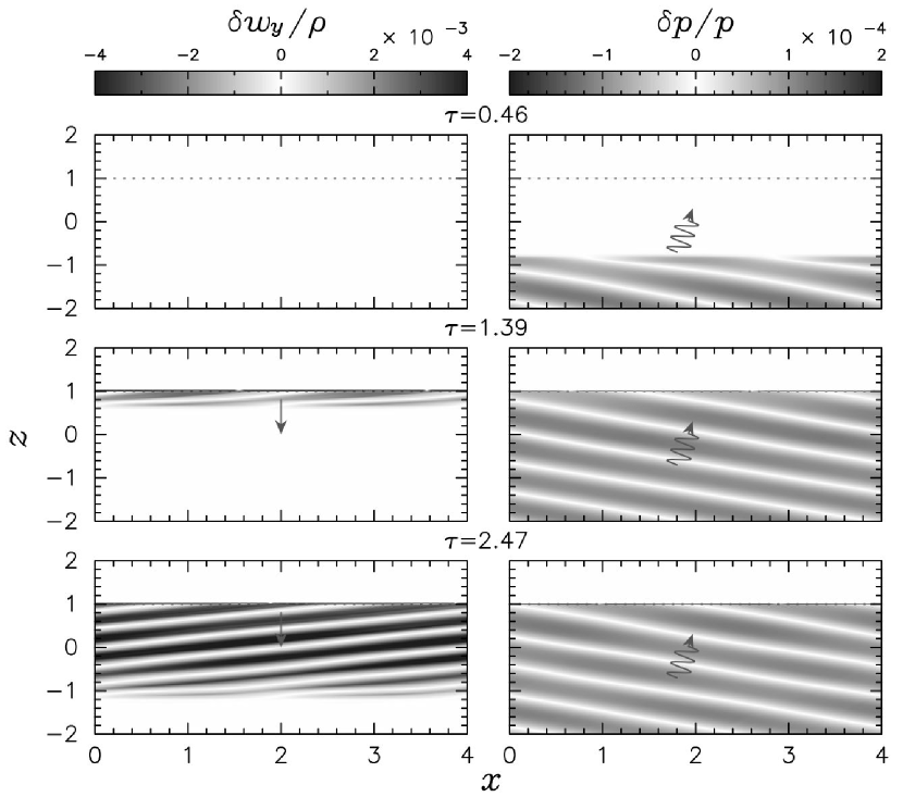
The snapshots in Fig. 2 show the specific vorticity $\delta w_{y}/\rho$ (left column) and pressure perturbation $\delta p/p$ (right column) in the flow at three successive times, before and after the moment when the advected wave reaches the deceleration region. The right column of Fig. 2 demonstrates the absence of an acoustic perturbation until the advected wave reaches the region of deceleration. Two acoustic waves are then generated, propagating upward and downward. This simple experiment gives a concrete illustration of the physical process described in analytical terms in paper I. In the bottom plots of Fig. 2, the flow has reached the asymptotic regime described by a single frequency in paper I, in which a more quantitative comparison of coupling efficiencies can be made. Since the computation domain is finite, the numerical experiment is stopped before the acoustic waves reach the vertical boundaries of the computation box in order to avoid spurious reflections. The time needed to reach the asymptotic regime described by a single frequency in paper I depends strongly on the frequency of the wave, and can become prohibitively long close to the frequency of horizontal propagation $\omega_{\rm ev}^{\rm in}$. This can be understood by viewing the semi-infinite acoustic plane wave, involved in both Problems 1 and 2, as an infinite plane wave of frequency $\omega_{0}$, multiplied by a step function, whose Fourier transform involves a continuum of frequencies. In 1-D, all frequencies would propagate with the same velocity, and the shape of the wave packet would stay unchanged during propagation. In 2D however, the high frequency part of the acoustic spectrum $\omega>\omega_{0}$ propagates more vertically than the main component, while the low frequency part $\omega_{0}>\omega>\omega_{\rm ev}^{\rm in}$ propagates more horizontally: this dispersion requires a longer numerical simulation, and thus a larger computational domain in order to avoid acoustic reflections. For this reason we have limited our investigation to the frequencies $\omega_{0}\tau_{\rm aac}/2\pi=1.5$, $2$, $4$, and $6$. Note that if the frequency of the perturbation had been chosen below the threshold of acoustic propagation ($\omega<\omega_{\rm ev}^{\rm in}$), the acoustic feedback would be evanescent above the deceleration region (paper I and Guilet, Sato & Foglizzo, in preparation).

3.2. Measure of the acoustic feedback in Problem 1

Figure 3.— Efficiency $(\hat{\delta p}_{0}/p_{\rm{in}})/\delta S$ of the production of acoustic waves by the deceleration of entropy/vorticity waves, measured at $z=0.5$, as a function of $\omega_{0}$ in Problem 1. The solid line shows the curve computed by a linear analysis (paper I). The results of numerical simulations are shown for different square mesh sizes $\Delta x=\Delta z=5\times 10^{-2}$ (crosses), $2\times 10^{-2}$ (triangles) and $10^{-2}$ (circles). The results for $\Delta x=2\times 10^{-2}$, $\Delta z=10^{-2}$ are also shown (pluses).

The amplitude of the acoustic feedback is measured in the numerical experiment by using a Fourier transform, in time, of the pressure perturbation over the period $T\equiv 2\pi/\omega_{0}$ of the wave:

$$\hat{\delta p}_{0}=\frac{2}{T}\int^{T}_{0}{\delta p}\;e^{i\omega_{0}t}dt,$$ (20)

The symbols in Fig. 3 are measured at $z=0.5$, in a region where the gravitational potential is uniform. The full line in Fig. 3 shows the expected efficiency $(\hat{\delta p}_{0}/p_{\rm in})/\delta S$ of the acoustic feedback obtained by integrating the differential system as in paper I. The good agreement with the perturbative calculation for a fine mesh (circles) confirms the validity of both the perturbative calculation and the numerical code. Given the long horizontal wavelength of the perturbations, the results are insensitive to an increase of the horizontal size $\Delta x$ of the mesh (pluses and circles). As described in paper I, the efficiency of the acoustic feedback decreases for frequencies above the cut-off $\omega_{\nabla}\sim 1/\tau_{\nabla}$.

3.3. Entropy/vorticity produced by a shock perturbed by an acoustic wave (Problem 2)

Figure 4.— Production of a vorticity wave by the interaction of an oblique acoustic wave with the shock (Problem 2). $\delta w_{y}/\rho$ (left) and $\delta p/p$ (right) are shown at three successive times, before and after the acoustic wave reaches the shock localised at $z=1$ (dashed line). A vorticity wave is generated and advected downward. The parameters are $\omega_{0}\tau_{\rm aac}/2\pi=2$, and $\Delta x=\Delta z=10^{-2}$.

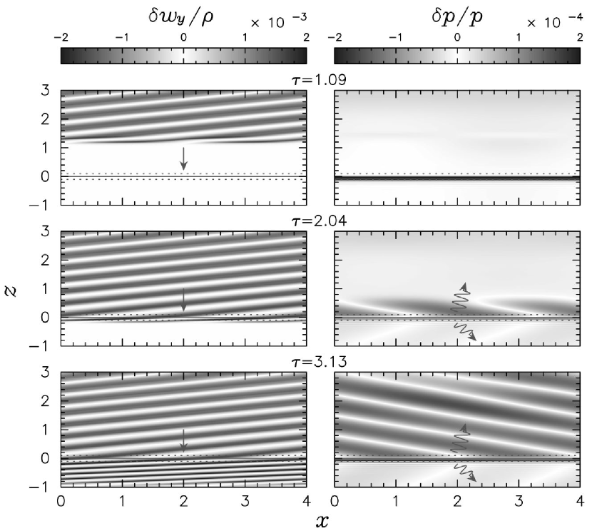
The upward propagation of the acoustic wave generated at the lower boundary of the computation domain in Problem 2 is visible on the right column of Fig. 4. The three snapshots illustrate the independence of advected and acoustic perturbations in the uniform part of the flow: the vorticity wave visible on the left column in Fig. 4 is generated only as the acoustic wave reaches the shock. This vorticity wave is then continuously generated by the shock and advected downward with the flow. An entropy wave (not shown) is also generated at the shock, with the same appearance as the vorticity wave. The lower boundary condition in this experiment is chosen far enough so that the reflected acoustic wave generated at the shock does not have time to interact with the lower boundary. The efficiency of entropy/vorticity generation at the shock can be measured at the time corresponding to the bottom panel in Fig. 4, and compared to the calculations of paper I.

3.4. Measure of the entropy production in Problem 2

Figure 5.— Dependence of $\hat{\delta S}_{0}/(\delta p/p_{\rm in})$, measured at $z=0.5$, on the frequency $\omega_{0}$, in Problem 2. The solid line shows curve predicted from linear analysis (paper I). The result of numerical simulations is shown for different mesh sizes $\Delta z=2\times 10^{-2}$ (pluses), $\Delta z=10^{-2}$ (squares), $5\times 10^{-3}$ (crosses), $2\times 10^{-3}$ (triangles) and $10^{-3}$ (circles) where $\Delta x=2\times 10^{-2}$. The filled points show the results for $\Delta x=\Delta z=10^{-2}$.

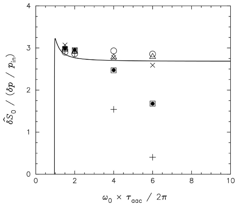
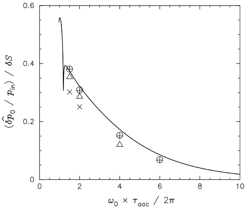
According to Eqs. (30-31) of paper I, the amplitude $\delta S_{\rm th}$ of the entropy wave produced by an acoustic wave reaching the shock is expected to be related to the frequency of the pressure wave as shown by the full line in Fig. 5:

$$\delta S_{\rm th}= \frac{\delta p}{p_{\rm in}}\;\;\frac{2}{\cal M_{\rm in}}\;\;\frac{1-{\cal M}_{\rm in}^{2}}{1+\gamma{\cal M}_{\rm in}^{2}}\left(1-\frac{{\cal M}_{\rm in}^{2}}{{\cal M}_{1}^{2}}\right)$$ (21)

$$\times\frac{\mu}{\mu^{2}+2\mu{\cal M}_{\rm in}+{\cal M}_{1}^{-2}}.$$

Measuring the amplitude of the entropy wave produced by the shock in the numerical simulations is not straightforward because of the presence of spurious high frequency oscillations, analysed in more details in the next section. We choose to measure (at $z=0.5$) its fundamental Fourier component $\hat{\delta S}_{0}$ at the frequency $\omega_{0}$, thus filtering out oscillations at higher frequency. The result is displayed in Fig. 5 for different frequencies and mesh sizes. We did not notice any dependence on the horizontal size $\Delta x$ of the mesh, for the long horizontal wavelengths considered. The expectation of the perturbative calculation is confirmed, but the convergence to the analytical formula is apparently much slower than for Problem 1. The rate of convergence is analysed in the next section using 1D simulations.

4. Accuracy of the numerical convergence

The dependence of the numerical error on the mesh size is easier to investigate using 1D simulations because of the shorter computation time. Without excluding the possibility of additional difficulties in 2D, we demonstrate here that some numerical difficulties associated to the advective-acoustic coupling are already present in 1D. The set up we use in this section is the same as used for the 2D simulations except that $k_{x}=0$.

4.1. Quadratic convergence in Problem 1

Figure 6.— Numerical error as a function of the mesh size for Problem 1. The panels (a), (b) and (c) correspond to the cases of $\omega_{0}\tau_{\rm aac}/2\pi=2$, $4$ and $6$, respectively. The dotted lines, proportional to $\Delta z^{2}$, illustrate the quadratic convergence.

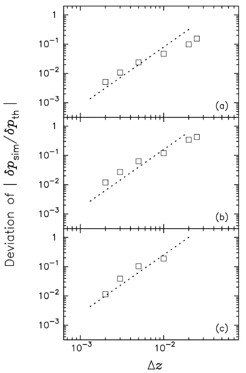
A series of numerical simulations of Problem 1 in 1D with different mesh sizes and perturbation frequencies allowed us to measure the accuracy of the computation compared to the perturbative analysis as shown in Fig. 6 by the open squares. They are to be compared with the dotted line, whose slope of $+2$ illustrates second order convergence for this problem. Remembering that the accuracy of our numerical scheme is second order in space, it is satisfactory to find that the error displayed in Fig. 6 is approximately quadratic with respect to the mesh size. The shortest wavelength in Problem 1 is the wavelength $2\pi v_{\rm out}/\omega_{0}$ of advected perturbations after their deceleration, which is equal to $\sim 0.12$ for the frequency $\omega_{0}\tau_{\rm aac}/2\pi=6$. We conclude from Fig. 6 that our numerical treatment of advection, propagation and advective-acoustic coupling involved in Problem 1 is accurate at the percent level even when the shortest wavelength is sampled by only $N\sim 10$ grid zones.

4.2. Linear convergence in Problem 2

Figure 7.— Time evolution of the amplitude of $\delta S/\delta S_{th}$ at $z=0.5$ for the same three frequencies as in Fig. 6. The thick line, dotted and thin lines correspond to the cases $\Delta z=10^{-2}$, $10^{-3}$ and $10^{-4}$, respectively.

Figure 8.— Numerical error of the quantity $|\hat{\delta S_{0}}/\delta S_{\rm th}|$ as a function of the mesh size for Problem 2. The frequencies are the same as in Fig. 6. The empty squares and filled circles were obtained with the AUSMDV scheme and the code RAMSES respectively. The dotted lines, proportional to $\Delta z$, illustrate the linear convergence.

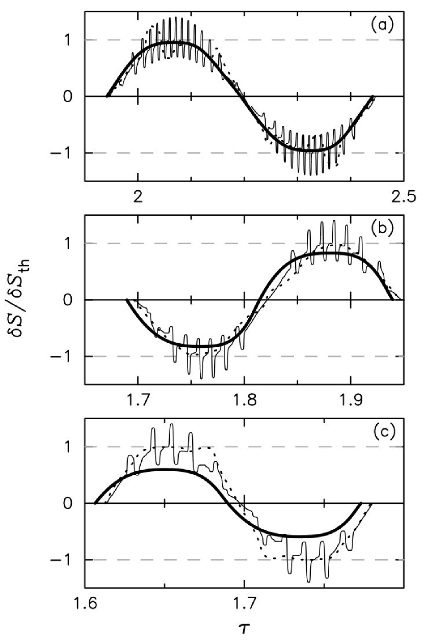
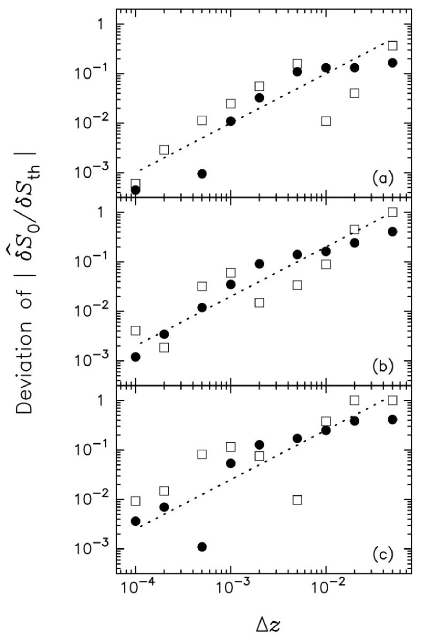
Applying the same test to Problem 2 is more complicated because of the high frequency oscillations already mentioned in Sect. 3. The shape of the entropy wave is shown in Fig. 7 for different frequencies and mesh sizes. The finer the mesh the higher the frequency of these spurious oscillations. We checked that the power involved in the Fourier component associated with these higher frequencies is always negligible compared to the main component. The Fourier component associated with the fundamental frequency $\omega_{0}$ converges slowly to the expected analytical value for a fine mesh. The squares in Fig. 8 show the numerical accuracy of the AUSMDV scheme for Problem 2, revealing a linear convergence with the mesh size (as shown by the dotted line of slope $+1$). We note that a coarse resolution can either underestimate or even overestimate the production of entropy at the shock. In order to show that this linear convergence is not a peculiarity of the AUSMDV scheme, these simulations were repeated with the code RAMSES. The results obtained with RAMSES are shown by the blacks circles in Fig. 8 (note that we also observed spurious high frequency oscillations in that case). They are comparable to those obtained using the AUSMDV scheme. Based on this comparison, we anticipate that all finite volume codes in which the treatment of the shock relies on an upwind technique are likely to share the same difficulty: quantities produced at the shock location, such as vorticity and entropy waves, or the reflected acoustic wave, are computed with a first order accuracy with respect to the mesh size. Likewise, we anticipate that all finite volume codes will suffer from the presence of spurious high frequency oscillations similar to those described above. It is indeed well known that such codes are subject to this problem, especially in the case of standing shocks, as was reported by Colella & Woodward (1984). In the present case, the problem is made worse by the interaction between the shock and the sound wave (in the absence of the latter, we barely detected high frequency oscillations, with an amplitude of the order of $0.5\%$ of the amplitude of the reflected entropy wave). As described by Colella & Woodward (1984), any additional source of dissipation (artificial viscosity, grid translation) will result in a decrease of the amplitude of the oscillations. For example, with RAMSES, the use of the Monotonised Central slope limiter (Toro, 1997), which is known to be less dissipative than MinMod, resulted in the amplitude of the oscillations being about three times larger. However, the complete stabilisation of the oscillations (through the use of artificial viscosity for example) would most probably come at the cost of reducing the growth rate, which we show in Sect. 5 not to be affected by the oscillations.

5. Eigenfrequency in the full toy model

Figure 9.— Growth rate $\omega_{i,\rm sim}$ and oscillation frequency $\omega_{r,\rm sim}$ of the most unstable mode ($n_{x}=1$) measured in a numerical simulation of the full toy model, compared to the values $\omega_{i,\rm th}$, $\omega_{r,\rm th}$ obtained from the perturbative analysis (paper I). The parameters are $L_{x}/H=4$, $H_{\nabla}/H=0.1$, ${\cal M}_{1}=5$, $c_{\rm in}^{2}/c_{\rm out}^{2}=0.75$, and $\Delta x=10^{-2}$. Perturbations were initiated with a random noise. Error bars are associated to the fitting procedure.

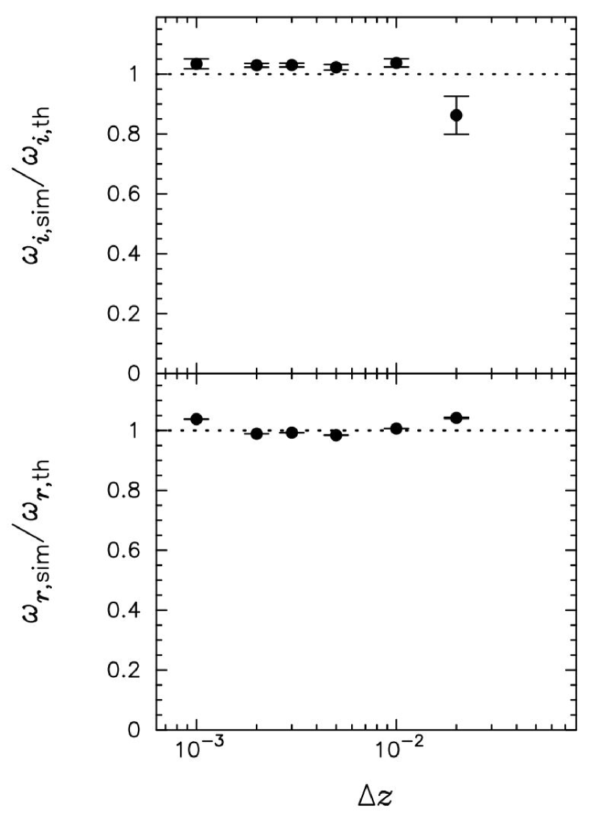
The full toy model has been simulated in order to measure the oscillation frequency $\omega_{r}$ and growth rate $\omega_{i}$ of the dominant eigenmode for ${\cal M}_{1}=5$, $H_{\nabla}/H=0.1$, $L_{x}/H=4$ and $c_{\rm in}^{2}/c_{\rm out}^{2}=0.75$. One difficulty for this simulation is the numerical relaxation of the unperturbed flow on the computational grid, which can result in a slow drift of the shock. The stationary flow is constructed by first obtaining a stationary subsonic flow in the gravitational potential, and then choose the upstream flow such that a shock is stationary at $z=z_{\rm sh}$. As a result of numerical discretization, the upstream mach number may slightly differ from ${\cal M}_{1}=5$, by a few percents. This difference is taken into account in the perturbative calculation of the reference eigenfrequency. Perturbations are incorporated as a random noise in the transverse velocity at the level of $10\%$ of the flow velocity in the uniform region between $z=0.3$ and $z=0.9$. The linear evolution is dominated by the mode $n_{x}=1$, as expected from the linear stability analysis. The comparison with the perturbative calculation is shown in Fig. 9. The oscillation frequency and growth rate, determined numerically, are accurate to about $5\%$ for $\Delta z\leq 10^{-2}$, suggesting that the spurious high frequency oscillations revealed in Sect. 3.4 and 4.2 have a minor effect on the eigenfrequency of the most unstable mode. The slight excess of the growth rate $\omega_{i,\rm sim}$ in Fig. 9 may be related to the fact that entropy and vorticity pertrubations are slightly overproduced at the shock, as seen in Fig. 5 for Problem 2. This effect, however, should be partially compensated by the slight underproduction of the acoustic feedback in Problem 1 (Fig. 3).
A significant damping of the instability ($\sim 14\%$) occurs if the grid is too coarse $(\Delta z=2\times 10^{-2})$ but even then, the oscillation frequency is accurate within $5\%$. The surprising accuracy of the oscillation frequency can be understood by the fact that the oscillation timescale is closely related to the timescale, for an advective-acoustic cycle between the shock and the deceleration region. Since the position of the acoustic feedback is set by the external potential in our toy model, this timescale barely depends on the numerical resolution. One must keep in mind that in a realistic flow where gradients are due to cooling processes, a change of numerical resolution could influence the position of the deceleration region, and could thus affect the oscillation timescale of the instability.

6. Consequences for core-collapse simulations

The results of our numerical experiments can be helpful to choose the mesh size in future simulations of a collapsing stellar core, both at the shock and near the neutron star, in order to make sure that the physics of SASI is correctly treated, at least in the linear regime. Of course, the influence of SASI on the mechanism of core-collapse supernovae depends on non-linear quantities such as the amplitude of the shock oscillations, the advection time through the gain region, or the spectral distribution of energy below the shock. Characterising which of the non-linear properties of SASI are most sensitive to the numerical technique is beyond the scope of the present study, and will be investigated in a forthcoming publication. We believe however that the coupling between entropy, vorticity and pressure is likely to play an important role even in the non linear regime of SASI, both through the flow gradients and at the shock. The wide range of frequencies involved in the non linear evolution of SASI (e.g. Yoshida et al. 2007) suggests that the accuracy of the numerical treatment should not be limited to the low frequency of the most unstable mode. In this sense, the numerical constraints deduced from our linear analysis should be considered as a minimum requirement, even-though some non-linear consequences of SASI may be less sensitive to numerical resolution than others: the addition of numerical errors with opposite signs, mentioned in Sect. 5, may contribute to the complex, non monotonic dependence of the explosion time with respect to the numerical resolution, observed by Murphy & Burrows (2008).

6.1. Mesh size in the deceleration region

When the shock stalls above the proto-neutron star, the flow deceleration close to the neutron star is dominated by cooling processes much more than by gravity, and the advective-acoustic coupling there is not adiabatic. By making the choice of simplicity, our toy model does not aim at reproducing quantitatively the efficiency of the acoustic feedback in a non-adiabatic flow. It helps understand that a simulation with a coarse grid in the vicinity of the neutron star may be unable to take into account a possible acoustic feedback from this region, simply because advected perturbations are numerically damped before reaching it. Let us consider a numerical simulation of an advective-acoustic cycle dominated by the oscillation frequency $\omega_{0}$. The choice of the mesh size close to the surface of the neutron star is not obvious because the wavelength of advected perturbations $\lambda_{\rm adv}\sim 2\pi v(r)/\omega_{0}$ shrinks as the gas is decelerated. Fortunately, an accurate advection of this perturbation is needed only down to the region where most of the acoustic feedback is generated, adiabatic or not. Since the timescale of the advective-acoustic cycle is larger than the advection timescale, and comparable to the oscillation timescale $2\pi/\omega_{\rm f}$ of the fundamental mode, the region of feedback is necessarily above the radius $r_{\rm in}$ reached by the gas during one SASI oscillation. According to Figs. 4 and 5 of FGSJ07, the dominant mode is the fundamental one ($\omega_{f}=\omega_{0}$) if the shock is close to the neutron star, or the first harmonic ($\omega_{f}\sim 2\omega_{0}$) if the shock distance is large enough. $r_{\rm in}$ is thus defined by:

$$\int_{r_{\rm in}}^{r_{\rm sh}}{{\rm d}r\over|v|}\equiv{2\pi\over\omega_{\rm f}}.$$ (22)

A possible strategy to choose the mesh size $\Delta r_{\rm in}$ in the inner region of the flow could be to make sure that the advected perturbations are correctly advected down to this radius $r_{\rm in}$. Denoting by $N$ the number of grid zones per wavelength required for an accurate advection and acoustic coupling of vorticity perturbations, the maximal mesh size $\Delta r_{\rm in}$ near the radius $r_{\rm in}$ should be

$$\Delta r_{\rm in}\equiv{1\over N}\;\;{2\pi\over\omega_{0}}v(r_{\rm in}).$$ (23)

Our illustration in Fig. 6 suggests $N\sim 10$. Of course, the precise value of $N$ depends on the numerical technique used and is expected to vary from code to code but is likely to remain of the same order as our estimate. In any case, Eq. (23) will be useful for future numerical simulations involving SASI, as a consistency check that the advective-acoustic feedback is properly resolved, at least for the fundamental mode.

6.2. Mesh size near the stalled shock

Figure 10.— Two-dimensional distribution of the power in the a fundamental mode, $|\hat{\delta S_{0}}/\delta S_{\rm th}|^{2}$, function of $\Delta\zeta/\Delta z$ and $\lambda_{\rm adv}/\Delta z$ obtained in the 1D simulations of problem 2.

Our study of Problem 2 has identified the difficulty of accurately calculating the entropy generated by the shock in a numerical simulations. This difficulty is likely to affect any physical quantity depending on the physics of the shock, such as the vorticity and the amplitude of reflected pressure waves. In this sense, all the numerical simulations of core-collapse involving SASI must face a similar difficulty with the numerical treatment of the shock.

We argue that this difficulty is not specific to the linear regime of the instability. In the non linear regime of SASI, as long as the shock continues to play a fundamental role by generating entropy and vorticity perturbations, the accuracy of the quantities depending on its behaviour are likely to be affected by this first order convergence. However, the details and precise consequences of this issue in that case remain an open issue at the present time. Answering these questions will require more realistic simulations, coupling both problems and carried to the non linear regime.

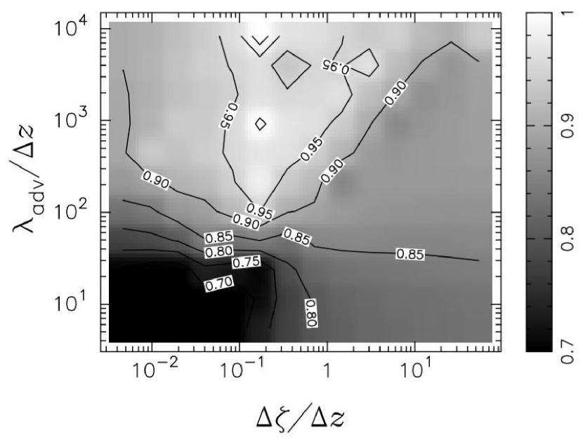
Should the grid size be able to resolve the displacement of the shock for a better accuracy ? According to the perturbative analysis, the shock displacement $\Delta\zeta$ is related to the entropy perturbation $\delta S$ by Eq. (16) of paper I:

$$\Delta\zeta=\left|\frac{c_{\rm in}^{2}}{\omega_{0}v_{1}}\;\;\frac{\delta S}{\gamma}\;\;\frac{1}{\left(1-v_{\rm in}/v_{1}\right)^{2}}\right|.$$ (24)

We show on Fig. 10 the accuracy of the numerical simulation, compared to the linear calculation, depending on how the grid sizes compares to both the shock displacement $\Delta\zeta$ and the advection wavelength $\lambda_{\rm adv}=2\pi\left|v_{\rm in}\right|/\omega_{0}$, in 1D calculations. Non linear effects become dominant for $\Delta\zeta>\lambda_{\rm adv}/100$. In the linear regime ($\Delta\zeta<\lambda_{\rm adv}/100$), an accuracy of $10\%$ requires $\Delta z<\lambda_{\rm adv}/100$. Resolving the shock displacement does not seem to be a crucial condition for the computation of the entropy production.

Since the exact properties of numerical convergence vary from a numerical scheme to another, it is not possible here to determine the real accuracy of existing numerical simulations involving SASI. At best we can estimate what would be the accuracy of our AUSMDV scheme in the conditions used by various authors. The mesh size $\Delta r_{\rm sh}$ at the radius of the stalled shock in published simulations varies depending on their complexity and the size of their outer boundary. We estimated $\Delta r_{\rm sh}\sim 1$ km in the 2D simulations of BM06 and Scheck et al. (2008), $\Delta r_{\rm sh}\sim 2$ km in Ohnishi et al. (2006) and Iwakami et al. (2008), and $\Delta r_{\rm sh}\sim 5$ km in Burrows et al. (2006). Estimating the value of the ratio $\lambda_{\rm adv}/\Delta r_{\rm sh}$ is possible by identifying $\omega_{0}$ with the oscillation frequency of the dominant mode. We estimated $\lambda_{\rm adv}/\Delta r_{\rm sh}\sim 200$ in BM06 and Scheck et al. (2008), which seems marginally sufficient to obtain a $10\%$ accuracy from the point of view of Fig. 10. The discrepancy of $30\%$, noted by FGSJ07 between the numerical results of BM06 and the perturbative analysis when the shock distance increases, may be related to the fact that the instability becomes dominated by the first harmonic rather than the fundamental mode. The correspondingly deeper coupling region may require a smaller mesh size, as already noted in FGSJ07 on the basis of the structure of the eigenfunction. Remembering that the mesh size in BM06 is one of the finest among the existing core-collapse simulations, particular attention on this issue seems necessary for the future simulations in which SASI could play an important role.

7. Conclusions

• A toy model has been used to illustrate through numerical experiments the coupling processes described in mathematical terms in paper I. Despite the high degree of simplification of our toy model, in particular the adiabatic hypothesis and the very local character of the deceleration region, these simulations can help us build our intuition about the physics of the advective-acoustic instability and better recognise it when present in numerical simulations.

• The results of the perturbative approach have been confirmed quantitatively by our numerical simulations.

• We have studied the effect of the mesh size on the accuracy of the numerical calculation. This will prove useful in the future to improve the reliability of the hydrodynamical part of simulations involving SASI in the core-collapse problem. We have proposed a conservative estimate of the desired mesh size close to the neutron star, which guarantees that the dominant acoustic feedback from advected perturbations is correctly taken into account.

• The difficulties associated with the numerical treatment of the shock have direct consequences on the accuracy with which the flow resulting from SASI is calculated: without a special numerical effort, the convergence of the computation of the growth time and oscillation frequency of SASI is reduced to first order even if the numerical scheme converges with a higher order away from the shock. Among the published simulations of SASI, only the 2D simulations with the finest grid seem to be able to estimate the entropy and vorticity production at the shock with a $<10\%$ accuracy. The importance of an accurate treatment of SASI in the core-collapse problem may make it worth implementing advanced techniques for the numerical treatment of the shock in future simulations, such as the level set method for example (Sethian & Smereka, 2003).

References

- Blondin et al. (2003) Blondin, J. M., Mezzacappa, A., & DeMarino, C. 2003, ApJ, 584, 971
- Blondin & Mezzacappa (2006) Blondin, J. M., & Mezzacappa, A. 2006, ApJ, 642, 401 (BM06)
- Blondin & Mezzacappa (2007) — 2007, Nature, 445, 58
- Burrows et al. (2006) Burrows, A., Livne, E., Dessart, L., Ott, C. D., & Murphy, J. 2006, ApJ, 640, 878
- Colella & Woodward (1984) Colella, P., & Woodward, P. R. 1984, J. Comput. Phys., 54, 174
- Foglizzo (2008) Foglizzo, T. 2008, submitted to ApJ (paper I)
- Foglizzo et al. (2007) Foglizzo, T., Galletti, P., Scheck, L., & Janka, H.-Th. 2007, ApJ, 654, 1006 (FGSJ07)
- Iwakami et al. (2008) Iwakami, W., Kotake, K., Ohnishi, N., Yamada, S., & Sawada, K. 2008, ApJ, 678, 1207
- Laming (2007) Laming, J. M. 2007, ApJ, 659, 1449
- Laming (2008) Laming, J. M. 2008, Erratum to be published in ApJ
- Liou & Steffen (1993) Liou, M. -S., & Steffen, C. J. 1993, J. Comput. Phys., 107, 23
- Marek & Janka (2007) Marek, A., & Janka, H.-Th. 2007, ApJ, submitted (arXiv: 0708.3372)
- Miyoshi & Kusano (2005) Miyoshi, T., & Kusano, K. 2005, JCoPh, 208, 315
- Murphy & Burrows (2008) Murphy, J. W., & Burrows, A. 2008, ApJ, 688, 1159
- Ohnishi et al. (2006) Ohnishi, N., Kotake, K., & Yamada, S. 2006, ApJ, 641, 1018
- Scheck et al. (2008) Scheck, L., Janka, H.-Th., Foglizzo, T., & Kifonidis, K. 2008, A & A, 477, 931
- Scheck et al. (2004) Scheck, L., Plewa, T., Janka, H.-Th., Kifonidis, K., & Müller, E. 2004, Phys. Rev. Lett., 92, 011103
- Sethian & Smereka (2003) Sethian, J.A., & Smereka, P., 2003, Annual Review of Fluid Mechanics, 35, 341
- Teyssier (2002) Teyssier, R., 2002, A&A, 385, 337
- Toro et al. (1994) Toro, E. F., Spruce, M., & Speares, W., 1994, Shock Waves, 4, 25
- Toro (1997) Toro, E. F., 1997, Riemann solvers and numerical methods for fluid dynamics (Springer)
- Wada & Liou (1994) Wada, Y., & Liou, M. S. 1994, AIAA Paper, 94-0083
- Yamasaki & Foglizzo (2008) Yamasaki, T., & Foglizzo, T. 2008, ApJ, 679, 607
- Yoshida et al. (2007) Yoshida, S., Ohnishi, N., & Yamada, S. 2007, ApJ, 665, 1268