Absolute Properties of the Spotted Eclipsing Binary Star CV Boötis

Abstract

We present new $V$-band differential brightness measurements as well as new radial-velocity measurements of the detached, circular, 0.84-day period, double-lined eclipsing binary system CV Boo. These data along with other observations from the literature are combined to derive improved absolute dimensions of the stars for the purpose of testing various aspects of theoretical modeling. Despite complications from intrinsic variability we detect in the system, and despite the rapid rotation of the components, we are able to determine the absolute masses and radii to better than 1.3% and 2%, respectively. We obtain $M_{\rm A}=1.032\pm 0.013$ M_☉ and $R_{\rm B}=1.262\pm 0.023$ R_☉ for the hotter, larger, and more massive primary (star A), and $M_{\rm B}=0.968\pm 0.012$ M_☉ and $R_{\rm B}=1.173\pm 0.023$ R_☉ for the secondary. The estimated effective temperatures are $5760\pm 150$ K and $5670\pm 150$ K. The intrinsic variability with a period $\sim$1% shorter than the orbital period is interpreted as being due to modulation by spots on one or both components. This implies that the spotted star(s) must be rotating faster than the synchronous rate, which disagrees with predictions from current tidal evolution models according to which both stars should be synchronized. We also find that the radius of the secondary is larger than expected from stellar evolution calculations by $\sim$10%, a discrepancy also seen in other (mostly lower-mass and active) eclipsing binaries. We estimate the age of the system to be approximately 9 Gyr. Both components are near the end of their main-sequence phase, and the primary may have started the shell hydrogen-burning stage.

1. Introduction

CV Boo (= BD +37 2641 = GSC 2570 0843; $\alpha=15^{\rm h}\,26^{\rm m}\,19\fs 54$, $\delta=+36\arcdeg\,58\arcmin\,53\farcs 4$, J2000.0; $V\approx 10.8$, SpT = G3V) was discovered as a possible eclipsing binary star by Peniche et al. (1985). Busch (1985) confirmed it as an eclipsing binary of type EA and found its period to be 0.8469935 days. In his last published paper, a study of 4 lower main sequence binaries, Popper (2000) determined a spectroscopic orbit for CV Boo. Popper was pessimistic about the prospects for determining accurate absolute properties of them because “It appears unlikely that definitive photometry will be obtained for these stars, partly because of intrinsic variability.” Recently, a light curve and radial velocity study of the system were done by Nelson (2004b), resulting in the first estimates of its absolute properties.

The parameters of CV Boo make it potentially interesting as the most evolved system among the well-studied double-lined eclipsing binaries with components near 1 M_☉ (see Figure 1), a regime where some discrepancies with theoretical models have been pointed out. We describe in the following our extensive new photometric and spectroscopic observations of the object intended to improve our knowledge of the system. The presence of starspots does in fact limit somewhat our ability to determine highly accurate absolute properties for this binary star, but the results are still accurate enough for meaningful tests of current stellar models. As we describe here, CV Boo contributes significantly to the body of evidence concerning the differences with theory mentioned above.

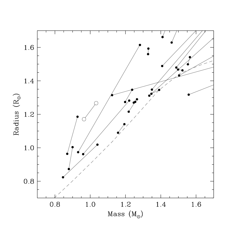
Figure 1.— Main-sequence eclipsing binaries in mass range of CV Boo with accurate determinations of their absolute properties (masses and radii good to better than $\sim$2%). Data are taken from Andersen (1991) and updates from the literature. Primary and secondary components are connected with solid lines. CV Boo is represented with open circles. The dashed line shows the solar-metallicity zero-age main sequence from the models by Yi et al. (2001), for reference.

2. Observations and reductions

2.1. Differential and absolute photometry

New differential brightness measurements of CV Boo were obtained with the facilities available at the Kimpel Observatory (ursa.uark.edu). They consist of a Meade 10-inch f/6.3 LX-200 telescope with a Santa Barbara Instruments Group ST8 CCD camera (binned 2$\times$2 to produce 765$\times$510 pixel images with 2.3 arcsec square pixels) inside a Technical Innovations Robo-Dome, controlled automatically by an Apple Macintosh G4 computer. The observatory is located on top of Kimpel Hall on the Fayetteville campus of the University of Arkansas, with the control room directly beneath the observatory inside the building. Sixty-second exposures through a Bessell $V$ filter (2.0 mm of GG 495 and 3.0 mm of BG 39) were read out and downloaded by ImageGrabber (camera control software written by J. Sabby) to the control computer over a 30-second interval, and then the next exposure was begun. The observing cadence was therefore about 90 s per observation. The variable star would frequently be monitored continuously for 4–8 hours. CV Boo was observed on 89 nights during parts of two observing seasons from 2001 December 1 to 2003 June 9.

The images were analyzed by a virtual measuring engine application written by Lacy that flat-fielded the images, automatically located the variable and comparison stars in the image, measured their brightnesses, subtracted the corresponding sky brightness, and corrected for the differences in airmass between the stars. Extinction coefficients were determined nightly from the comparison star measurements. They averaged 0.20 mag/airmass. CV Boo is also known as GSC 2570 0843. The comparison stars were GSC 2570 0511 (“comp”, $V=10.26$, as listed in the Tycho Catalogue), and GSC 2570 0423 (“ck”). Both comparison stars are within 8 arcmin of the variable star (“var”). The comparison star magnitude differences $\langle$comp$-$ck$\rangle$ were constant at the level of 0.013 mag (standard deviation within a night), and 0.007 mag for the standard deviation of the nightly mean magnitude difference. The differential magnitude $\langle$var$-$comp$\rangle$ of the variable star was referenced only to the magnitude of the comparison star, comp. The resulting 6500 $V$-band magnitude differences $\langle$var$-$comp$\rangle$ are listed in Table 1 and plotted in Figure 2. The typical precision of the variable star differential magnitudes is about 0.013 mag per measurement.

In addition to our own, differential photometry of CV Boo was obtained by Nelson (2004b) in $V$ and Cousins $I$ between 2003 March and June (253 and 265 measurements, respectively). The comparison star was GSC 2570 0869, and the check star was GSC 2570 0511, which is the same star we used as the comparison. These observations are incorporated into our analysis below.

Absolute photometry of CV Boo is available in the literature from several sources, and color indices can be used to estimate a mean effective temperature for the combined light of the system (assuming no interstellar reddening). The results are collected in Table 2. We used the color/temperature calibrations of Ramírez & Meléndez (2005) for dwarf stars for all but the Sloan $g\!-\!r$ index; for that color we used the calibration of Girardi et al. (2004). In all cases we assumed solar metallicity. The value of Johnson $V$ is that listed in the Tycho Catalogue with no uncertainty given there. We have assumed a conservative error of 0.10 mag for $V$. The temperature estimate from the Johnson $B\!-\!V$ index uses the value of that index as listed in the Tycho Catalogue, with its listed error. The temperature values estimated in these ways agree quite well, except for the estimates from $B\!-\!V$ and $B_{\rm T}\!-\!V_{\rm T}$, which happen to have the largest formal errors. The weighted average of the 7 estimates is $5706\pm 60$ K, where the uncertainty does not account for possible systematic errors in the various calibrations. This color-index-based temperature is quite consistent with spectroscopic estimates discussed below, and this suggests that the interstellar reddening value, if any, is very small.

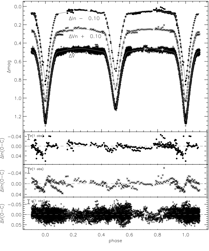
Figure 2.— The top panel shows our $V$-band light curve of CV Boo ($+$ symbols), consisting of 6500 points, together with the $V$ ($\times$) and $I$ ($\bullet$) light curves from Nelson (2004b), marked “$\Delta V$n” and “$\Delta I$n”. Nelson’s light curves are shifted as indicated, for clarity. Our theoretical solution without spots is overplotted (continuous grey lines; § 3.1). The lower panels show the $O\!-\!C$ residuals from these fits, and in the upper left corner, the standard deviation for a single measurement.

CV Boo is identified as a strong X-ray source in the ROSAT catalog (Voges et al., 2000). This is presumably due to an active chromosphere/corona associated with its spot activity (see below).

2.2. Ephemeris

Photoelectric or CCD times of minimum light for CV Boo carried out over the past decade have been reported by a number of authors (Agerer & Hübscher, 2002, 2003; Bakis et al., 2003; Diethelm, 2001; Dogru et al., 2006; Hübscher, 2005; Hübscher et al., 2005, 2006; Kim et al., 2006; Lacy, 2002, 2003; Maciejewski & Karska, 2004; Nelson, 2000, 2002, 2004a). Additional times of eclipse including older visual and photographic measurements reaching back to 1957 were kindly provided by J. M. Kreiner (see Kreiner, Kim & Nha, 2000) or taken from the literature (Locher, 2005; Molik, 2007). Separate least-squares fits to the 98 available primary and 50 secondary minima yielded ephemerides with virtually the same period within the errors. A simultaneous fit to all minima was then performed assuming a circular orbit. Uncertainties were initially adopted as published, or assigned by iterations and by type of observation so as to achieve a reduced $\chi^{2}$ of unity. The resulting linear ephemeris is

$${\rm Min~{}I~{}(HJD)}=2,\!452,\!321.845322(50)+0.846993420(69)E.$$ (1)

where the figures in parentheses represent the uncertainty in units of the last decimal place. No significant trends indicative of period changes are seen in the $O\!-\!C$ residuals. A test solving for separate primary and secondary epochs with a common period yielded a phase difference between the eclipses of $\Delta\phi=0.49991\pm 0.00013$. This is consistent with 0.5, supporting our earlier assumption of a circular orbit.

2.3. Spectroscopy

CV Boo was observed spectroscopically with an echelle instrument on the 1.5m Tillinghast reflector at the F. L. Whipple Observatory (Mt. Hopkins, Arizona). A total of 66 spectra were gathered from 1991 June to 2005 April, each of which covers a single echelle order (45 Å) centered at 5188.5 Å and was recorded using an intensified photon-counting Reticon detector. The strongest lines in this window are those of the Mg I $b$ triplet. The resolving power of this setup is $\lambda/\Delta\lambda\approx 35,\!000$, and the observations have signal-to-noise ratios ranging from 13 to 36 per resolution element of 8.5 km s^-1.

Radial velocities were obtained using the two-dimensional cross-correlation algorithm TODCOR (Zucker & Mazeh, 1994). Templates for the cross correlations were selected from an extensive library of calculated spectra based on model atmospheres by R. L. Kurucz (see also Nordström et al., 1994; Latham et al., 2002). These calculated spectra cover a wide range of effective temperatures ($T_{\rm eff}$), rotational velocities ($v\sin i$ when seen in projection), surface gravities ($\log g$), and metallicities. Experience has shown that radial velocities are largely insensitive to the surface gravity and metallicity adopted for the templates, as long as the temperature is chosen properly. Consequently, the optimum template for each star was determined from extensive grids of cross-correlations varying the temperature and the rotational velocity, seeking to maximize the average correlation weighted by the strength of each exposure. Solar metallicity was assumed. The results, interpolated to surface gravities of $\log g=4.25$ for both stars (see § 3), are $T_{\rm eff}=5800$ K and $v\sin i=73$ km s^-1 for the primary star, and $T_{\rm eff}=5650$ K and $v\sin i=67$ km s^-1 for the secondary. Estimated uncertainties are 200 K and 10 km s^-1 for the temperatures and projected rotational velocities, respectively. Template parameters near these values were selected for deriving the radial velocities. Typical uncertainties for the velocities are 5.6 km s^-1 for the primary and 5.9 km s^-1 for the secondary, which are considerably worse than usual with this instrument because of the significant rotational broadening of both stars.

The stability of the zero-point of our velocity system was monitored by means of exposures of the dusk and dawn sky, and small run-to-run corrections were applied in the manner described by Latham (1992). Additional corrections for systematics were applied to the velocities as described by Latham et al. (1996) and Torres et al. (1997) to account for residual blending effects and the limited wavelength coverage of our spectra. These corrections are based on simulations with artificial composite spectra processed with TODCOR in the same way as the real spectra. The final heliocentric velocities are listed in Table 3.

The light ratio between the components was estimated directly from the spectra following Zucker & Mazeh (1994). After corrections for systematics analogous to those described above, we obtain $\ell_{\rm B}/\ell_{\rm A}=0.71\pm 0.04$ at the mean wavelength of our observations (5188.5 Å), where we refer to star A as the more massive one (the primary) and to the other as star B. This value is in reasonable agreement with estimates by Popper (2000) based on the relative strength of the Na I D lines in CV Boo. Given that the stars have slightly different temperatures (see below), a small correction to the visual band was determined from synthetic spectra integrated over the $V$ passband and the spectral window of our observations. The corrected value is ($\ell_{\rm B}/\ell_{\rm A})_{V}=0.73\pm 0.04$.

Radial velocities for CV Boo have been reported previously also by Popper (2000), who observed the star as part of his program focusing on binary systems of spectral type F to K. His 45 measurements from 1988 February to 1997 June with the Hamilton spectrometer at the Lick Observatory partially overlap in time with ours, and are of excellent quality. However, they require a number of adjustments before they can be combined with ours. One of these adjustments has to do with corrections he applied to his raw velocities. The raw velocities (which he referred to as “Observed”) were reported for CV Boo alongside “Orbital” velocities which differ from the raw ones by the application of two corrections. The first is analogous to the corrections for systematic effects we applied to our own velocities, and was derived in a similar manner using synthetic binary spectra (for details see Popper & Jeong, 1994). The second correction accounts for distortions and mutual irradiation in the close orbit, and was computed by Popper (2000) using the formalism developed by Wilson (1990) as implemented in the Wilson-Devinney (WD) program that we also use below, and added to the velocities. Given our plan to use the WD program to combine the light curves with the velocity measurements in a simultaneous solution, the latter corrections in the data by Popper (2000) need to be removed prior to use or they would be applied twice. We estimated these corrections from a preliminary solution with WD (presumably emulating Popper’s procedure), and applied them with the opposite sign to the “Orbital” velocities. These corrections are no larger than 1 km s^-1, which is smaller than the formal uncertainties in the velocities (2.7 km s^-1 for the primary and 2.1 km s^-1 for the secondary, from the residuals of preliminary fits).

A second adjustment we found necessary to apply to Popper’s measurements is to correct for an offset of 1.60 km s^-1 between his primary and secondary velocities, as indicated by preliminary sine-curve fits (see Table 6 by Popper, 2000, where the offset he finds is similar). Effectively the two stars yield different center-of-mass velocities. We found no such offset in our own measurements, but experience indicates it can sometimes appear when there is a significant mismatch between the adopted templates and the real stars, and if not corrected it can bias the semi-amplitudes when enforcing a common center of mass in the fit. We have thus added $-1.60$ km s^-1 to Popper’s secondary velocities. Finally, a third adjustment is to bring Popper’s overall velocity zero point into agreement with ours. From trial orbital fits we found this required a shift of +0.37 km s^-1 to his velocities. Popper’s corrected velocities are listed in Table 4. Separate fits to his data and ours give similar values for the semi-amplitudes, and yield masses that differ by less than twice their combined uncertainties. We therefore proceed to merge the two data sets below.

A third set of radial velocities for CV Boo was reported by Nelson (2004b), but they were obtained at lower resolution, they are few in number (12), and show a much larger scatter than the two other data sets ($\sim$15 km s^-1) so they are of little use for our purposes.

3. Modeling of the photometric observations

The overall shape of CV Boo’s light curves (Figure 2) shows rather moderate proximity effects despite the system’s relatively short period of slightly more than 20 hours, with the curvature between the minima being mostly due to the deformation of the components and, to a smaller degree, to the mutual illumination. A number of small-scale features are obvious to the eye that are possibly due to spots, other intrinsic variability, or even instrumental effects, especially in the smaller data sets of Nelson (2004b). Other features described below are revealed through a more detailed examination, and introduce some complications into the analysis.

3.1. Initial solutions without spots

To begin with, we chose to model all the observations together in order to obtain a baseline solution against which to compare more complex solutions that attempt to account for the features mentioned above. We used a version of the Wilson-Devinney (WD) modeling program (Wilson & Devinney, 1971; Wilson, 1979, 1993) with extensive modifications as described in Vaz, Andersen & Claret (2007) and references given therein. The modifications pertinent to CV Boo include the capability to use model atmospheres (now also available in the distributed versions of WD), consistency checks between various parameters, and the ability to use the downhill simplex algorithm (Nelder & Mead, 1965) instead of differential corrections. We combined our own $V$-band light curve with the sparser $V$ and $I$ light curves of Nelson (2004b) in order to improve the constraint on the effective temperature ratio, and with our radial velocities from § 2.3 as well as those of Popper (2000). Thus we solved simultaneously 3 light curves and 4 radial-velocity curves. The parameters adjusted were the orbital inclination $i$, the secondary $T_{\rm eff}$ (flux-weighted mean surface temperature), the bandpass-specific primary luminosity (see Wilson, 1993), both stellar surface gravitational pseudo-potentials $\Omega$ (related to the stellar radii), the center-of-mass radial velocity $\gamma$, the mass ratio $q\equiv M_{\rm B}/M_{\rm A}$, and an arbitrary phase shift. The similar depths of the two minima in both $V$ and $I$ (Figure 2) imply that the components must have rather similar temperatures, consistent with indications from spectroscopy. The primary temperature was held fixed at a value determined from our results based on photometry and spectroscopy, as follows. A photometric estimate of the primary temperature was derived from the mean system temperature (§ 2.1) using approximate values for the radius ratio and temperature ratio from preliminary light-curve solutions. The result, $5755\pm 60$ K, was then combined with the spectroscopic value of the primary temperature (§ 2.3), giving a weighted average for Star A of $5760\pm 150$ K, which we adopt.

The reflection albedos for both components were held fixed at the value 0.5, appropriate for stars with convective envelopes, and the gravity-brightening exponents $\beta$ were computed internally in WD using the local value of $T_{\rm eff}$ for each point on the stellar surface taking into account mutual illumination, following Alencar & Vaz (1997) and Alencar et al. (1999). The flux from each of the components is represented by NextGen atmosphere models based on the PHOENIX stellar atmosphere code (Allard & Hauschildt, 1995; Allard et al., 1997; Hauschildt et al., 1997a, b). The luminosity of the secondary is calculated by the program from its size and $T_{\rm eff}$. The limb-darkening coefficients for both components, $x_{\rm A}$ and $x_{\rm B}$, were taken from the tables by Claret (2000), and interpolated using a bi-linear scheme for the current values of $\log g$ and $T_{\rm eff}$ at each iteration. We have only considered the linear law here in view of the distortions in the light curve, which will tend to overwhelm the rather subtle effect of limb-darkening. Although we have no evidence of another star in the system, the possibility of third light ($\ell_{3}$) was explored carefully for its potential influence on the geometric parameters, particularly in the solutions described below in § 3.2, which include spots. Achieving convergence when solving for third light was found to be very difficult due to the intrinsic variability and the large number of free parameters, even when considering multiple parameter subsets (Wilson & Biermann, 1976). We found that the solution was not improved, and $\ell_{3}$ was not considered further. We estimate a conservative upper limit to $\ell_{3}$ of $\sim$1%, which does not produce significant changes in the geometric parameters. A circular orbit has been assumed in the following, based on our investigation of the eclipse timings in § 2.2, and the lack of any indication in the light curves of a displacement of the secondary minimum from phase 0.5. This is consistent with expectations from tidal theory for an orbit with such a short period (see § 6). We have also assumed here tidal forces have synchronized the components’ rotation with the orbital motion of CV Boo. In these initial calculations we applied both least-squares differential corrections and/or the simplex method between successive iterations. The limb-darkening coefficients, normalization magnitudes, surface gravities, and individual velocity amplitudes were all updated between consecutive runs to correspond to the solution from the previous iteration.

Figure 3.— Primary ($\times$) and secondary ($+$) radial velocity measurements collected at CfA (Table 3) along with the theoretical curves obtained with WD and no spots (top panel). Velocities are shifted so that the center-of-mass velocity $\gamma$ is at zero (dashed line). The large deviation from Keplerian motion in the predicted velocity around both conjunctions is due to the Rossiter-McLaughlin effect (see Schlesinger, 1909a, b; Rossiter, 1924; McLaughlin, 1924), caused by partial eclipses of the rotating stellar surfaces (an effect built into the WD model). The $O\!-\!C$ residuals are shown at the bottom. The standard deviation of the unweighted residuals is $\sigma_{\rm rv}=6.09$ km s^-1 for both components and is shown in the upper left corner. The reduced $\chi^{2}$ values were 1.000 and 0.998, respectively.

The solutions are shown in Figures 2, 3 and 4, with the corresponding residuals. The residuals from the radial velocity fits match the quality of the observations. The photometry is reasonably well represented on average by the theoretical curves, but the residuals for our $V$-band observations show an rms scatter of 0.0196 mag that is much larger than the mean internal error ($\sim$0.013 mag). This immediately suggests there may be unmodeled effects. The intrinsic errors of Nelson’s observations were not reported in the original publication.

Figure 4.— Primary ($\times$) and secondary ($+$) radial velocity data from Popper (2000), with the same limits on the vertical axes as in Figure 3. The standard deviations of the unweighted residuals are $\sigma_{\rm rv,A}=3.14$ km s^-1 and $\sigma_{\rm rv,B}=2.14$ km s^-1 for the primary and secondary velocities, respectively (shown in the upper left corner of the lower panels). The reduced $\chi^{2}$ values were 1.005 and 1.002.

3.1.1 Study of the light-curve residuals

Part of the extra scatter is no doubt due to features in the light curve alluded to earlier that are seen in Figure 2, such as changes in the light level from night to night at the same orbital phase (e.g., near phase 0.1), or other short-term deviations (e.g., near phase 0.8), both in our data and in Nelson’s. We investigated the residuals of our more numerous $V$-band photometry further to search for periodic signals that might additionally contribute to the excess scatter. Our initial exploration of possible signals near the orbital period using the Lafler & Kinman (1965) method revealed several similar periodicities that appear significant. We then extended the search to a much wider range of frequencies by computing the Lomb-Scargle periodogram, and found other signals. This is shown in the top panel of Figure 5. We refer to this as the “dirty” power spectrum, since it is affected by the particular time sampling of the observations (window function). The highest peak corresponds to a period of $\sim$0.837 days, which is shorter than the orbital period of 0.846993420 days. The two next highest peaks (indicated with arrows) turn out to be 1-day aliases. To illustrate this, we have applied the CLEAN algorithm as implemented by Roberts et al. (1987) to remove the effects of the window function. The second panel of Figure 5 shows that only the 0.837-day peak survives this process, suggesting it is a real signal. In the third panel an enlargement of the dirty power spectrum in the vicinity of the main peak reveals fine structure that was also seen with the Lafler & Kinman (1965) method. However, none of these peaks agree with the frequency corresponding to the orbital period, which is represented for reference with a dotted line. The two main sidelobes indicated with arrows are 1-year aliases of the main peak. Once again they disappear after application of CLEAN, as seen in the bottom panel, supporting the reality of the remaining signal. The statistical significance of this signal was estimated by numerical simulation. We generated $100,\!000$ artificial data sets using the actual times of observation and the variance of the original residuals assuming a Gaussian distribution of errors, and computed the Lomb-Scargle power spectrum for these data sets over the same frequency interval considered above. We then selecting the highest peak in each case. None of them came close to the height of the peak we see in the real data, indicating a false alarm probability smaller than $10^{-5}$.

Figure 5.— (a) Lomb-Scargle power spectrum of the residuals of our $V$-band Kimpel Observatory observations of CV Boo from the no-spot solution described in the text. The arrows indicate 1-day aliases of the central peak; (b) CLEANed power spectrum of the same measurements using the algorithm of Roberts et al. (1987) to remove the effects of the time sampling; (c) Enlargement of panel (a), with the 1-year aliases of the main peak indicated with arrows. The dotted line represents the orbital frequency; (d) Enlargement of panel (b). The period corresponding to the signal is $0.83748\pm 0.00052$ days.

The precise frequency of this signal was measured in the CLEANed spectrum, and its uncertainty was estimated from the half width at half maximum of the peak. The corresponding period is $0.83748\pm 0.00052$ days, which is different from the orbital period at the 18$\sigma$ level. A plot of the photometric residuals folded with this period is shown in Figure 6, and indicates a peak-to-peak amplitude of about 0.04–0.05 mag.

Figure 6.— Residuals of our $V$-band Kimpel Observatory observations of CV Boo shown as a function of phase, using the period of 0.83748 days inferred from the power spectrum analysis (see Figure 5). The time origin has been set arbitrarily to HJD $2,\!450,\!000$.

The Kimpel Observatory data cover two observing seasons. Separate Lomb-Scargle power spectra show that the same signal is present in both seasons, along with the 1-day aliases, indicating the phenomenon is persistent from one year to the next. It is not seen as clearly, however, in the residuals from our baseline fit of the observations of Nelson (2004b), which are much sparser than ours (and span only 71 days instead of 549 days). His $V$-band data show a hint of the main peak and its 1-day aliases, but not the $I$-band data, which have a larger scatter.

We carried out a similar power spectrum analysis of the $\langle$comp$-$ck$\rangle$ differential magnitudes from Kimpel Observatory, to explore the possibility that either the comparison or the check star might be the source of this variation. No significant periodicity was seen. Thus, the phenomenon is intrinsic to CV Boo. Possible explanations for this variation include stellar pulsation, and star spots on one or both components. Neither of the stars appear to be in an evolutionary state that favors pulsational instability. For example, the absolute dimensions derived below place both components well outside the Cepheid or $\delta$ Sct instability strips in the H-R diagram indicated by Kjærgaard et al. (1983). On the other hand, CV Boo is a known strong X-ray source detected by ROSAT (Voges et al., 2000), with an X-ray luminosity of $\log L_{\rm X}=30.65$ that is some 4000 times stronger than the Sun. In terms of its bolometric luminosity CV Boo has $\log L_{\rm X}/L_{\rm bol}=-3.39$, which is near the high end for active binaries. Thus it seems likely that the underlying reason for the 0.837-day periodicity is related to spots on the surface of one or both components, and we proceed under this assumption. It is interesting to note that these features on CV Boo seem to have lasted for an unusually long time (1.5 years in our case), at least compared to sunspots, although even more extreme examples have been documented in the literature. One is the well-known active binary HR 1099 (Vogt et al., 1999), with surface features persisting for at least 11 years.

An important implication of this spot hypothesis is that the component having spots would appear to be rotating slightly more rapidly than synchronously with the motion in the circular orbit, which is unexpected for such a short-period binary. We discuss this in more detail below.

3.2. Solutions with spots

An accurate measurement of the $v\sin i$ values for both components would allow for a direct test of our hypothesis of non-synchronous rotation, and could even distinguish which of the stars is the culprit (or if both are). Unfortunately, however, the quality of our spectroscopic material is insufficient for that purpose. In principle, modern light-curve models such as WD enable the user to solve for various parameters that describe the spots. However, with only photometric data at our disposal for CV Boo, and most of it in a single passband, it is essentially impossible to tell which star has the spots, or whether both components have them. This is a well-known difficulty in light-curve modeling. Other inversion techniques such as Doppler imaging are much better suited to mapping surface inhomogeneities, although even they are not without their limitations. Moreover, even if we knew which star has the spots, the determination of their parameters from light curves alone is a notoriously ill-posed problem, on which there is abundant literature discussing issues of indeterminacy and non-uniqueness in the presence of limited data quality (see, e.g., Eker, 1996, 1999, and numerous references therein). Having photometry in multiple passbands may aleviate the problem somewhat, but it doesn’t solve it and strong degeneracies are likely to remain with other subtle effects in the light-curves. Therefore, while we cannot hope to obtain an accurate picture of the distribution of any surface features here, the consequences of spots on the light curve are fairly clear in CV Boo (to the extent that our hypothesis is true), and we make an effort in the following to at least remove some of those distortions and study their influence on the geometric parameters of the system, which are of more immediate interest.

In order to permit the numerical treatment of surface features in this case, we introduced modifications in the WD code to allow for a precise tracking of the spot position at a period different than the orbital one. In this scheme, we specify the spot properties at a certain Julian date and, through the specified intrinsic rotation rate, the code keeps track of the spot motion, with its longitude following the component’s rotation, and its co-latitude, size, and effective temperature remaining otherwise constant. In view of the ambiguities mentioned above regarding the location of spots in CV Boo, and our inability to tell if there might even be multiple spots on one or both stars, we have taken our light-curve fit from § 3.1 as our starting point and investigated the following three simple cases separately: (a) a single spot on the primary; (b) a single spot on the secondary; and (c) one spot on each component. More complex configurations become increasingly difficult to study due to convergence problems in the solutions, and it is not clear they are justified with the data available.

The influence of spots on the radial velocity curves is very small compared to our errors, so that those data are not of very helpful for studying surface features. We use only our more extensive $V$-band photometry in the study of these three cases, although the solutions were checked using Nelson’s $V$ and $I$ light curves. As the photometric coverage does not necessarily overlap with the radial velocity coverage, we have adopted for the spotted cases the mass ratio $q$ obtained from a no-spot fit similar to that in § 3.1 that assumes asynchronous rotation (see below), and held it fixed. For lack of other physical constraints, and given that the stars are quite similar in all their properties, we assumed that both components rotate slightly super-synchronously, at a rate given by the ratio between the orbital period and the residual period found in the previous section, equal to 1.0114.

Cases (a) and (b) converged quite rapidly to similar configurations, in which the co-latitude, size, and the effective temperatures of the spots are comparable, while their longitudes are such that the spots present always the same position relative to the center of the spotted component and the observer. This can be seen in Table 5, where the longitudes of the spots in cases (a) and (b) are separated by nearly 180$\arcdeg$. Another similarity is that both spots cover the components’ polar regions. Although attempted, no solution could be obtained for “hot” spots (i.e., with temperature factors larger than unity; see below).

Solution (c) with one spot on each component did not converge as easily. When the parameters of both spots were left free to be adjusted, one of the spots (usually the one on the primary) tended to become very small and cold, with the temperature factor $T_{\rm factor}$ (ratio between the spot temperature and the photospheric temperature) becoming smaller than allowed by the NextGen atmosphere tables we used. The solution we present was achieved by first adjusting some of the spot parameters while holding others fixed, and then alternating and iterating until convergence.

The maximum amplitude of the influence of the spots on the light curve is $\sim$0.08 mag, and occurs for the one-spot solutions, as shown in Figure 7. This figure corresponds to the first orbital cycle of our observations and, since the spots follow the components’ non-synchronous rotation, the dips change place at each orbiting cycle. The two-spot solution of case (c) gives a slightly smaller peak-to-peak amplitude ($\sim$0.06 mag) that seems marginally larger than indicated in Figure 6, suggesting that perhaps a more complex spot configuration may be needed.

Figure 7.— Difference between the light curves with spots and those without spots (shown in Figure 2), for the first cycle of our observations. The thin horizontal line shows the normalization level of the theoretical light curves (phase 0.25, first orbiting cycle).

We report in Table 6 the model parameters we obtain for the solution with no spots and for cases (a), (b), and (c), together with the radii of the components in terms of the orbital separation. For the reasons described above, the solution without spots was performed by solving simultaneously three light curves and 4 radial velocity curves, whereas the spotted fits are based only on our $V$-band light curve. The main difference in the parameter values is seen in the inclination angle, which is approximately one degree higher for the solution without spots. Other parameters such as the secondary effective temperature and the sizes of the components tend to differ less between the spotted and unspotted solutions.

Figure 8 gives a representation of the spot configuration resulting from case (c) with the components’ size and separation rendered to scale, and seen from the observer’s viewpoint at six different orbital phases. The stars are well detached from the corresponding Roche lobes, with fill-out factors (Mochnacki, 1984) that are 0.7693 and 0.7501 for the primary and secondary, respectively. We noted above that our fits yield polar spots, as has often been found (also from Doppler imaging techniques) for other active binaries such as the RS CVn systems. There is considerable theoretical support for this preference for high-latitude surface features in rapidly-rotating active systems (see, e.g., Schüssler & Solanki, 1992; Granzer et al., 2000; Işik et al., 2007). A curious result from our fits is that the spots happen to be positioned so as to avoid eclipses, although the reality of this configuration is difficult to assess. It is nevertheless an indication that the phenomenon responsible for the periodic behavior of the residuals in the unspotted solution does not lead to strong discontinuities, such as those resulting from the eclipses.

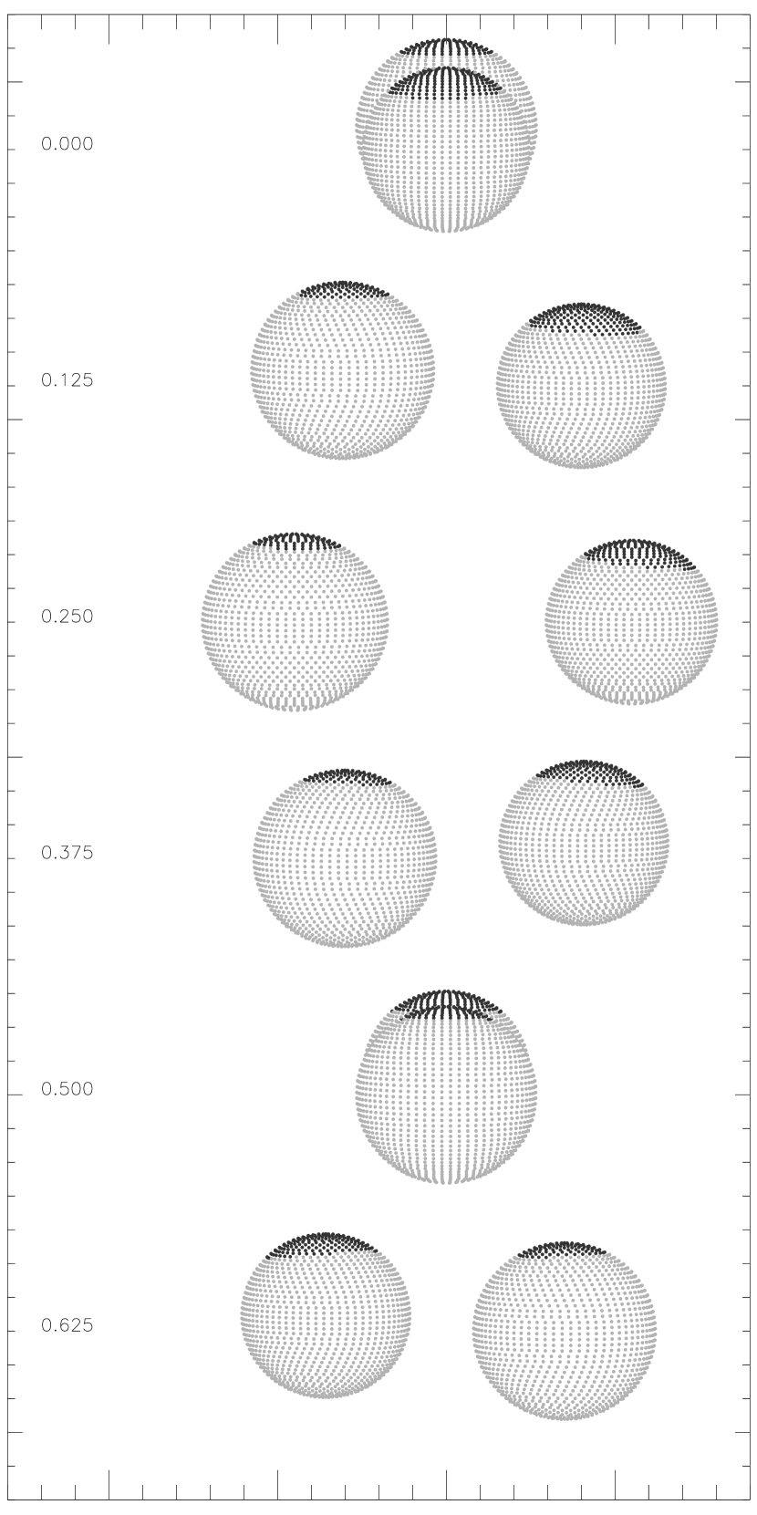
Figure 8.— Representation of the components of CV Boo at different orbital phases as indicated on the left, shown to scale with their high-latitude spots as modeled here. These spots resulting from our solution (c) are positioned in such a way that they practically avoid being eclipsed. This is an indication of a rather sinusoidal behavior of the disturbing phenomenon causing periodic variations in the residuals of the unspotted solution (see text).

Although the rms residual is marginally smaller for the solution obtained in case (c), as indicated in Table 6, this fit as well as the other two spotted solutions are visually indistinguishable from the solution without spots shown in Figure 2. The residuals for case (c) are displayed in Figure 9 for our $V$-band light curve as well as for the $V$ and $I$ light curves of Nelson (2004b). The patterns clearly visible in these $O\!-\!C$ diagrams are not very different from those in Figure 2, which may give the impression that not much progress has been made. They certainly indicate that there are still features of the brightness variation that are not completely or correctly modeled, possibly due to a more complex spot configuration than we have assumed, or even some combination of spots and multi-modal pulsations. Problems of an instrumental nature in the photometry cannot entirely be ruled out either. However, what is not immediately obvious to the eye is that no significant periodicities that we can detect remain in these residuals. This is illustrated in Figure 10, in which the top curve shows our Lafler-Kinman period study of the Kimpel Observatory $V$-band residuals from the no-spot solution, and the lower curve shows the same study for the residuals from case (c). Note the common vertical axis for both sets of residuals, indicating the improvement in the overall variance.

Figure 9.— $O\!-\!C$ residuals from the solution with one spot on each component, based on the fit to our $V$-band light curve. The model used to compute the residuals for the $V$ and $I$ light curves of Nelson (2004b) in the top panels is based on the same light-curve parameters as our $V$-band fit, except for the magnitude at quadrature and the wavelength of the observations. The standard deviation of a single observation for each residual curve is shown in the upper left corner of each panel.

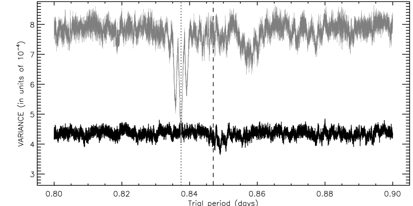
Figure 10.— The variance versus trial period in days (following Lafler & Kinman, 1965) for the Kimpel Observatory $V$-band residuals of the no-spot solution (top curve, corresponding to the fit shown in Figure 2), and for the solution with two spots (bottom curve; see text). The dotted line marks the most significant period found for the $O\!-\!C$ of the solution with no spots, while the dashed line indicates the orbital period.

4. Absolute dimensions and physical properties

Examination of Table 6 shows that key geometric parameters such as the relative radii ($r_{\rm A,vol}$, $r_{\rm B,vol}$) vary by as much as 3–4% between the three spotted solutions, with solution (c) generally giving intermediate results. As indicated earlier, this is the fit that provides formally the smallest rms residual, although the difference compared to the other two spotted solutions is marginal. In all four solutions the mean light ratio outside of eclipse accounting for spots, $(\ell_{\rm B}/\ell_{\rm A})_{V}$, is quite similar to the spectroscopically determined value of $0.73\pm 0.04$ (§ 2.3). From the effective temperatures of CV Boo A and B the convective turnover time for both stars is estimated to be $\sim$25 days, following Hall (1994). The Rossby number (ratio between the rotation period and the convective turnover time) is then $R_{0}\approx 0.033$, which places both components in the regime where stars usually display significant light variations due to spots (see Hall, 1994, Figure 6). On the basis of the above we adopt fit (c) with one spot on each component as the best compromise for CV Boo, but we reiterate that this model is still probably only a crude approximation to the true spot configuration in the system, assuming that spots are the underlying reason for the periodic signal found in the light-curve residuals. For calculating the absolute dimensions of the two stars we have chosen to use more conservative uncertainties than the formal errors listed in Table 6, to account for the spread among the three spotted solutions given the uncertainties in the modeling: we have combined the internal errors quadratically with half of the maximum range in each parameter. The values adopted are $i=86\fdg 24\pm 0\fdg 33$, $a=4.748\pm 0.019$ R_☉, $q=0.9378\pm 0.0070$, $r_{\rm A,vol}=0.2658\pm 0.0047$, and $r_{\rm B,vol}=0.2470\pm 0.0048$, and are based only on the Kimpel Observatory measurements. The final results are presented in Table 7, where the uncertainties were obtained by propagating all observational errors in the usual way.

The stars in CV Boo depart somewhat from the spherical shape due to tidal and rotational distortions. The relative difference between the polar radius and the radius toward the inner Lagrangian point is 5.5% for the primary and 4.8% for the secondary. The system is nevertheless well detached: the sizes of the stars represent fractions of 70% and 66% of their respective mean Roche lobe sizes. The temperature for the secondary from the light-curve solution is in excellent agreement with the spectroscopic value (§ 2.3).

Included in Table 7 are the predicted projected rotational velocities ($v_{\rm async}\sin i$) computed with the adopted rotation period for the stars ($P_{\rm rot}=0.83748$ days $=P_{\rm orb}/1.0114$; see § 3.1.1), as well as the synchronous values ($v_{\rm sync}\sin i$), for reference. These may be compared with the measured $v\sin i$ values from spectroscopy (§ 2.3). The stellar radii used for these calculations are those presented to the observer at quadrature (which are 2.7% and 2.4% larger than the volume radii; see Table 6), since that is the phase at which the spectroscopic observations are concentrated. As a proxy for the radius at quadrature we use the average of $r_{\rm point}$ and $r_{\rm back}$.

Finally, for computing the absolute visual magnitude $M_{V}$ and distance we have relied on the apparent $V$ magnitude listed in the Tycho Catalog, and ignored extinction. CV Boo was not observed by the Hipparcos mission (Perryman et al., 1997), so no direct parallax measurement is available.

5. Comparison with stellar evolution theory

In this section we compare the absolute dimensions of CV Boo with current stellar evolution models from the Yonsei-Yale series by Yi et al. (2001), incorporating an updated prescription for convective core overshooting as described by Demarque et al. (2004). These models adopt a mixing length parameter of $\alpha_{\rm ML}=1.7432$, calibrated against the Sun. In Figure 11 we show evolutionary tracks computed for the exact masses we derive for each star (see Table 7), for a heavy-element abundance equal to that of the Sun (which is $Z_{\sun}=0.01812$ in these models; dotted lines). The uncertainty in the location of the tracks that comes from our mass errors is indicated with the error bar in the lower left. The tracks show excellent agreement with the observations, suggesting the composition is near solar. The measured temperature difference between the components is quite close to what the models predict. A marginally better match is achieved with a slightly higher abundance of $Z=0.01955$ (corresponding to [Fe/H] $=+0.04$, assuming no enhancement of the $\alpha$ elements), shown as solid lines in the figure. The models indicate the primary is beginning its shell hydrogen-burning phase, and the secondary is near the end of its main-sequence phase. The age that best fits both components in this $\log g$–$T_{\rm eff}$ diagram is $9.0\pm 1.8$ Gyr, and the corresponding isochrone is shown as a dashed line.

Figure 11.— Absolute dimensions for CV Boo compared with evolutionary models from the series by Yi et al. (2001). The error bars for $\log g$ are smaller than the size of the symbols. Mass tracks for the exact masses we measure are indicated with solid curves for the best-fitting metallicity of $Z=0.01955$ (where $Z_{\sun}=0.01812$ for these models). Solar metallicity tracks are shown for reference (dotted curves). The isochrone producing the best simultaneous match to both components is shown with the short-dash line, and corresponds to an age of 9.0 Gyr. The long-dash lines represent small sections of the two isochrones corresponding to the maximum and minimum age allowed by the errors ($9.0\pm 1.8$ Gyr). The uncertainty in the location of the mass tracks is indicated with the error bar below the tracks for the primary, and is much smaller than the temperature uncertainty.

We have also considered a second set of models, from the series by Claret (2004). The physics in these calculations is similar though not exactly the same as the previous ones. For example, the solar composition in this case is taken to be $Z_{\sun}=0.020$, and the mixing length parameter that best reproduces the observed properties of the Sun is $\alpha_{\rm ML}=1.68$. The comparison with the observations for CV Boo is shown in Figure 12. Although the Claret models match the measured properties very well, we find as with the Yonsei-Yale models that a slightly higher metallicity ($Z=0.0225$, or [Fe/H] = $+0.05$) provides an even better fit. This is shown by the solid lines in Figure 12. The age of the system from these calculations is 9.8 Gyr, consistent with the previous estimate. Experiments changing the mixing length parameter show the sensitivity of the best-fit composition to $\alpha_{\rm ML}$. In Figure 13 we compare the observations with tracks computed for a lower value of $\alpha_{\rm ML}=1.50$, which has the effect of yielding lower temperature predictions. Solar-metallicity models are indicated with the dotted lines. In this case we find that the best-fit metallicity ($Z=0.0185$, or [Fe/H] $=-0.03$) is slightly lower than solar (solid lines).

Figure 12.— Absolute dimensions for CV Boo compared with evolutionary models from the series by Claret (2004) with a value of the mixing-length parameter of $\alpha_{\rm ML}=1.68$. Mass tracks for the exact masses we measure and for solar composition ($Z=0.020$, $X=0.70$, in these models) are indicated with dotted curves. The solid curves giving a somewhat better fit correspond to models with a slightly higher metallicity of $Z=0.023$. An isochrone for $\log$ age = 9.99 is shown for reference (dashed line). The uncertainty in the location of the mass tracks is indicated with the error bar below the tracks for the primary, and is much smaller than the temperature uncertainty.

The preceding comparisons may give the impression that the observations for CV Boo are very well matched by the predictions from theory, that stellar physics is well understood, and that therefore there is no reason for concern. However, a more careful examination indicates that this is not necessarily true. Of the three basic parameters typically determined in eclipsing binaries ($M$, $R$, $T_{\rm eff}$), the temperature is usually the weakest since it often relies on external calibrations. Figure 14 displays the measurements for CV Boo in a different diagram, the mass-radius plane, along with isochrones from the Yonsei-Yale series for the same two metallicities discussed in Figure 11. No single model matches both components within the errors, and the secondary appears nominally older than the primary, the difference in age being $\sim$25%. This is the same phenomenon pointed out by Popper (1997) for several other systems including FL Lyr, RT And, UV Psc, and $\alpha$ Cen. Another way of interpreting this is that the secondaries in all these binaries are too large for their masses, compared to theory or compared to the primaries. For CV Boo the offset in the secondary radius is $\sim$10%, which represents a very significant 5$\sigma$ deviation. Similar radius discrepancies have been described recently by others (e.g., Clausen et al., 1999a; Torres & Ribas, 2002; Ribas, 2003; López-Morales & Ribas, 2005; Torres, 2007), although early indications go as far back as the work of Hoxie (1973) and Lacy (1977). The prevailing explanation seems to be that the enlarged radii of the secondaries, which are typically well under a solar mass, are caused by strong magnetic fields and/or spots commonly associated with chromospheric activity in these systems (see, e.g., Mullan & MacDonald, 2001; Chabrier et al., 2007, for the theoretical context). The signs of activity in CV Boo are fairly obvious (spottedness, X-ray emission), and are no doubt associated with the rapid rotation of the components.

Figure 13.— Same as Figure 12, but for a mixing-length parameter of $\alpha_{\rm ML}=1.50$. Mass tracks for the measured masses and for solar composition ($Z=0.020$, $X=0.70$) are indicated with dotted curves. The somewhat better-fitting solid curves correspond to a slightly lower metallicity of $Z=0.0185$ in this case, showing the influence of the $\alpha_{\rm ML}$ parameter in the determination of the composition of CV Boo.

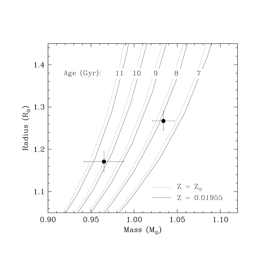
Figure 14.— Mass-radius diagram for CV Boo, showing the measurements against isochrones from the Yonsei-Yale series for the same two metallicities displayed in Figure 11. Ages are indicated along the top.

6. Comparison with tidal theory

The predictions of tidal theory were compared with the observations by computing the time of circularization and synchronization for CV Boo using the radiative damping formalism of Zahn (1977) and Zahn (1989), as well as the hydrodynamical mechanism of Tassoul & Tassoul (1997), and references therein. The procedure follows closely that described by Claret et al. (1995) and Claret & Cunha (1997). Both theories predict that synchronization and circularization are achieved very quickly in this system by virtue of the short orbital period, at an age of merely 157 Myr ($\log t=8.197$, or less than 2% of the evolutionary age). The fact that we measure the orbit to be circular is therefore not surprising. On the other hand, the evidence from our photometric observations (§ 3.1.1) suggesting the rotation may be slightly super-synchronous for at least one of the components is more interesting, as it is not predicted by theory. Given the nature of the system, an activity-related explanation to this discrepancy is certainly possible. More precise measurements of the projected rotational velocities $v\sin i$ for the components would be very helpful.

7. Discussion and conclusions

Despite the system’s intrinsic variability, the absolute dimensions for the components of CV Boo have now been established quite precisely. The relative errors are better than 1.3% in the masses and 2% in the radii. The object can now be counted among the group of eclipsing binaries with well-known parameters. Under different circumstances the large number and high quality of the photometric observations we have collected might have permitted a more detailed study of the limb darkening laws and a comparison with theoretically predicted coefficients, but this possibility was thwarted here by the intrinsic variability. This phenomenon is not itself without interest. If interpreted as due to the presence of spots, as we have done here, it implies that at least one of the stars is rotating about 1% more rapidly than the synchronous rate, a result that was unexpected for a close but well detached system such as this. We conclude that our current understanding of tidal evolution is still incomplete, or that other processes are at play in this system that theory does not account for. One interesting possibility is differential rotation. The interpretation of measurements of the rotation period of a star made by photometric means, as we have implicitly done here, usually relies on the assumption of solid-body rotation. More often than not, spots are located at intermediate latitudes rather than on the equator, or at high latitudes in more active stars, and differential rotation is such that the stellar surface revolves more slowly at higher latitudes, at least in the Sun. This will tend to bias photometric rotation measurements towards longer periods, if differential rotation is significant enough. In CV Boo we see the opposite: the period is shorter than the equatorial rate, assuming that synchronization holds. Thus differential rotation can only explain the signal we have detected if it is “anti-solar”, with the polar regions rotating more rapidly. A handful of stars do indeed show evidence of weak anti-solar differential rotation (e.g., IL Hya, HD 31933, $\sigma$ Gem, UZ Lib; Weber et al., 2003; Strassmeier et al., 2003; Kõvári et al., 2007; Vida et al., 2007). They all happen to be very active (some of them with high-latitude spots, as in CV Boo), although they tend to be giants or subgiants rather than dwarfs. It is thought that this phenomenon may result from fast meridional flows (see, e.g., Kitchatinov & Rüdiger, 2004). Further progress in understanding the rotation of the CV Boo components could be made with additional differential photometric observations in several passbands, along with simultaneous high-resolution, high signal-to-noise ratio spectroscopy over a full orbital cycle.

Another significant discrepancy we find with theory is in the radius of the secondary, which appears to be some 10% too large compared with predictions from stellar evolution models. This difference is in the same direction as seen for a number of other low-mass eclipsing binaries, as mentioned in § 5. In those cases one of the explanations most often proposed is that the strong magnetic fields associated with activity (which is common in rapidly-rotating K and M dwarfs in close binaries) tend to inhibit convective motions, and the structure of the star adjusts by increasing its size to allow the surface to radiate the same amount of energy. At the same time, the effective temperature tends to decrease in order to preserve the total luminosity. Spot coverage can produce similar effects. Theoretical and observational evidence for the conservation of the luminosity in these systems has been presented by Delfosse et al. (2000), Mullan & MacDonald (2001), Torres & Ribas (2002), Ribas (2006), Torres et al. (2006), Chabrier et al. (2007), and others (see also Morales et al., 2008). We do not see any obvious discrepancy in the temperature of CV Boo B compared to models, although our uncertainties are large enough that the effect may be masked.

If we restrict ourselves to well studied double-lined eclipsing binaries in which the mass and radius determinations are the most reliable, deviations from theory such as those described above have usually been seen in stars that are considerably less massive than the Sun, which have deep convective envelopes. However, the recent study by Torres et al. (2006) pointed out that the problem is not confined to the lower mass stars, but extends to active objects approaching 1 M_☉, such as V1061 Cyg Ab, with $M=0.93$ M_☉. CV Boo B has an even larger mass of 0.968 M_☉, and also appears to be oversized. Similarly with the virtually identical active star FL Lyr B ($M=0.960$ M_☉). The convective envelopes of these objects are considerably thinner than in K and M dwarfs and represent only a few percent of the total mass, yet they appear sufficient for magnetic fields to take hold and alter the global properties of the star, if that is the cause of the discrepancies. These examples show once again that our understanding of stellar evolution theory is incomplete, even for stars near the mass of the Sun.

Table 1Differential $V$-band measurements of CV Boo.

HJD$-2,\!400,\!000$	Phase	$\Delta V$
52250.99816	0.35467	+0.452
52250.99907	0.35575	+0.416
52251.00000	0.35685	+0.445
52251.00091	0.35792	+0.508
52251.00182	0.35900	+0.433

Note. — Table 1 is available in its entirety in the electronic edition of the Astronomical Journal. A portion is shown here for guidance regarding its form and contents.

Table 2Photometric indices and inferred mean effective temperature of CV Boo.

Photometric Index	Value	$T_{\rm eff}$ (K)	Ref.
Johnson $V$	10.75 $\pm$ 0.100	$\cdots$	1
Johnson $B\!-\!V$	0.73 $\pm$ 0.11	5417 $\pm$ 350	1
Tycho-2 $B_{\rm T}-V_{\rm T}$	0.82 $\pm$ 0.13	5448 $\pm$ 329	1
Johnson/2MASS $V\!-\!J$	1.18 $\pm$ 0.10	5693 $\pm$ 103	1,2
Johnson/2MASS $V\!-\!H$	1.47 $\pm$ 0.10	5666 $\pm$ 155	1,2
Johnson/2MASS $V\!-\!K_{s}$	1.55 $\pm$ 0.10	5692 $\pm$ 157	1,2
Tycho-2/2MASS $V_{\rm T}-K_{s}$	1.629 $\pm$ 0.081	5679 $\pm$ 129	1,2
Sloan $g\!-\!r$	0.473 $\pm$ 0.002	5760 $\pm$ 100	3

Note. — References: (1) Høg et al. (2000); (2) Cutri et al. (2003); (3) Sloan Digital Sky Survey data.

Table 3New radial velocity measurements of CV Boo.

${{\mathrm{HJD}}\atop{-2\,440\,000}}$	Phase	${{\displaystyle\mathrm{Star~{}A}}\atop{\mathrm{km/s}}}$	${{\mathrm{(O\!-\!C)}}\atop{\mathrm{A}}}$	${{\displaystyle\mathrm{Star~{}B}}\atop{\mathrm{km/s}}}$	${{\mathrm{(O\!-\!C)}}\atop{\mathrm{B}}}$	${{\mathrm{HJD}}\atop{-2\,440\,000}}$	Phase	${{\displaystyle\mathrm{Star~{}A}}\atop{\mathrm{km/s}}}$	${{\mathrm{(O\!-\!C)}}\atop{\mathrm{A}}}$	${{\displaystyle\mathrm{Star~{}B}}\atop{\mathrm{km/s}}}$	${{\mathrm{(O\!-\!C)}}\atop{\mathrm{B}}}$
48408.8881	0.1792	$-$127.53	$-$2.12	$+$144.05	$+$13.68	52805.7304	0.2974	$-$133.61	$-$1.12	$+$134.43	$-$3.53
48428.7637	0.6453	$+$113.28	$+$6.33	$-$121.89	$-$4.64	52807.6959	0.6180	$+$79.11	$-$12.00	$-$96.25	$+$4.12
48435.7679	0.9148	$+$70.53	$+$1.73	$-$80.45	$-$4.19	52808.6829	0.7833	$+$141.29	$+$8.91	$-$158.46	$-$14.00
52336.9667	0.8530	$+$101.70	$-$6.29	$-$121.62	$-$3.39	52828.6620	0.3715	$-$116.79	$-$16.14	$+$112.11	$+$8.13
52362.8251	0.3826	$-$96.29	$-$2.48	$+$97.00	$+$0.31	52830.7704	0.8608	$+$104.81	$+$0.97	$-$115.59	$-$1.81
52391.8515	0.6526	$+$115.23	$+$4.57	$-$126.58	$-$5.38	52894.6202	0.2449	$-$148.22	$-$9.80	$+$145.71	$+$1.37
52395.7780	0.2884	$-$126.96	$+$7.58	$+$131.35	$-$8.81	53011.0543	0.7124	$+$138.93	$+$7.38	$-$147.38	$-$3.84
52419.8759	0.7395	$+$133.04	$-$1.97	$-$156.34	$-$9.07	53017.0656	0.8097	$+$130.12	$+$4.16	$-$144.86	$-$7.31
52420.8446	0.8832	$+$80.62	$-$9.96	$-$102.38	$-$2.82	53036.0482	0.2214	$-$130.15	$+$6.19	$+$149.26	$+$7.14
52424.9263	0.7022	$+$119.97	$-$9.29	$-$137.99	$+$3.09	53045.0203	0.8143	$+$110.06	$-$14.40	$-$137.98	$-$2.03
52481.7239	0.7601	$+$131.60	$-$3.44	$-$147.89	$-$0.59	53047.9883	0.3184	$-$133.81	$-$7.71	$+$138.58	$+$7.46
52537.6015	0.7319	$+$145.12	$+$10.69	$-$153.73	$-$7.10	53072.0214	0.6931	$+$120.32	$-$6.41	$-$138.36	$+$0.02
52657.0283	0.7327	$+$136.61	$+$2.10	$-$143.34	$+$3.38	53102.9332	0.1890	$-$128.08	$+$0.67	$+$140.61	$+$6.65
52681.9996	0.2150	$-$139.26	$-$3.99	$+$149.89	$+$8.92	53124.9836	0.2227	$-$148.22	$-$11.69	$+$142.32	$-$0.01
52687.0564	0.1853	$-$126.70	$+$0.86	$+$125.61	$-$7.06	53125.8812	0.2825	$-$135.40	$+$0.26	$+$136.82	$-$4.54
52688.0019	0.3016	$-$136.00	$-$4.61	$+$134.21	$-$2.57	53131.8024	0.2733	$-$148.17	$-$11.15	$+$142.70	$-$0.12
52690.9568	0.7903	$+$137.79	$+$6.78	$-$152.45	$-$9.46	53133.8280	0.6648	$+$113.70	$-$2.64	$-$125.78	$+$1.49
52712.0278	0.6677	$+$117.71	$+$0.12	$-$132.03	$-$3.42	53134.8008	0.8134	$+$123.52	$-$1.25	$-$134.88	$+$1.40
52718.9482	0.8383	$+$103.39	$-$11.69	$-$126.31	$-$0.46	53155.9103	0.7362	$+$135.62	$+$0.82	$-$159.54	$-$12.50
52720.9903	0.2493	$-$142.32	$-$3.84	$+$135.44	$-$8.97	53156.8078	0.7959	$+$124.95	$-$4.81	$-$145.87	$-$4.23
52721.8866	0.3075	$-$131.97	$-$2.26	$+$135.59	$+$0.61	53157.6883	0.8354	$+$118.15	$+$1.81	$-$128.87	$-$1.66
52743.0017	0.2370	$-$138.96	$-$0.91	$+$141.72	$-$2.22	53158.8651	0.2248	$-$132.66	$+$4.16	$+$136.23	$-$6.41
52743.8681	0.2599	$-$138.48	$-$0.26	$+$136.36	$-$7.76	53159.7571	0.2779	$-$137.36	$-$0.97	$+$141.77	$-$0.38
52745.9296	0.6938	$+$127.96	$+$1.02	$-$152.37	$-$13.76	53182.6826	0.3449	$-$107.94	$+$7.08	$+$117.19	$-$2.10
52748.8870	0.1854	$-$124.72	$+$2.87	$+$133.76	$+$1.05	53183.7214	0.5713	$+$55.26	$-$2.71	$-$66.52	$+$2.40
52751.9548	0.8074	$+$122.44	$-$4.20	$-$141.35	$-$3.07	53183.8170	0.6842	$+$118.57	$-$5.32	$-$136.77	$-$1.44
52752.8104	0.8176	$+$118.39	$-$4.95	$-$137.92	$-$3.18	53184.7284	0.7602	$+$139.79	$+$4.76	$-$147.31	$-$0.01
52769.7356	0.8003	$+$123.65	$-$5.00	$-$141.11	$-$0.66	53189.7763	0.7200	$+$134.61	$+$1.70	$-$150.90	$-$5.90
52771.8062	0.2449	$-$139.56	$-$1.14	$+$137.19	$-$7.15	53190.6836	0.7912	$+$129.10	$-$1.72	$-$146.12	$-$3.34
52773.8521	0.6604	$+$103.84	$-$10.53	$-$124.10	$+$1.06	53192.6964	0.1676	$-$123.51	$-$2.64	$+$140.40	$+$14.92
52800.6851	0.3407	$-$116.42	$+$0.57	$+$128.81	$+$7.42	53217.6764	0.6602	$+$113.85	$-$0.42	$-$123.95	$+$1.11
52802.6741	0.6890	$+$120.03	$-$5.45	$-$138.94	$-$1.90	53452.8782	0.3505	$-$114.77	$-$2.51	$+$115.01	$-$1.34
52804.7941	0.1920	$-$127.64	$+$2.03	$+$145.25	$+$10.30	53485.8782	0.3118	$-$121.62	$+$6.74	$+$125.58	$-$7.96

Note. — The $O\!-\!C$ residuals correspond to the solution described in § 3.1.

Table 4Radial velocities for CV Boo from Popper (2000).

${{\mathrm{HJD}}\atop{-2\,440\,000}}$	Phase	${{\displaystyle\mathrm{Star~{}A}}\atop{\mathrm{km/s}}}$	${{\mathrm{(O\!-\!C)}}\atop{\mathrm{A}}}$	${{\displaystyle\mathrm{Star~{}B}}\atop{\mathrm{km/s}}}$	${{\mathrm{(O\!-\!C)}}\atop{\mathrm{B}}}$	${{\mathrm{HJD}}\atop{-2\,440\,000}}$	Phase	${{\displaystyle\mathrm{Star~{}A}}\atop{\mathrm{km/s}}}$	${{\mathrm{(O\!-\!C)}}\atop{\mathrm{A}}}$	${{\displaystyle\mathrm{Star~{}B}}\atop{\mathrm{km/s}}}$	${{\mathrm{(O\!-\!C)}}\atop{\mathrm{B}}}$
47198.0795	0.6418	$+$100.59	$-$4.51	$-$112.85	$+$2.43	49117.9386	0.3175	$-$126.53	$-$0.09	$+$133.81	$+$2.32
47254.9417	0.7760	$+$134.29	$+$0.77	$-$144.43	$+$1.25	49202.6852	0.3733	$-$102.13	$-$2.52	$+$101.37	$-$1.49
47397.6592	0.2749	$-$137.69	$-$0.88	$+$142.48	$-$0.12	49204.7213	0.7772	$+$133.70	$+$0.35	$-$145.93	$-$0.43
47695.7285	0.1895	$-$129.31	$-$0.39	$+$136.69	$+$2.54	49204.7416	0.8012	$+$126.62	$-$1.79	$-$140.09	$+$0.10
47696.7035	0.3407	$-$112.58	$+$4.42	$+$121.75	$+$0.35	49204.7623	0.8256	$+$117.42	$-$2.96	$-$130.86	$+$0.69
48080.7574	0.7727	$+$134.39	$+$0.45	$-$144.60	$+$1.53	49496.9018	0.7392	$+$135.56	$+$0.57	$-$147.61	$-$0.36
48081.6981	0.8833	$+$87.15	$-$3.33	$-$98.55	$+$0.90	49496.9163	0.7563	$+$134.71	$-$0.49	$-$146.30	$+$1.18
48312.0038	0.7931	$+$128.21	$-$2.20	$-$139.74	$+$2.60	49583.6596	0.1695	$-$126.79	$-$5.13	$+$126.42	$+$0.08
48344.9980	0.7476	$+$131.13	$-$4.16	$-$144.15	$+$3.42	49583.6807	0.1944	$-$128.99	$+$1.40	$+$132.75	$-$2.98
48345.8895	0.8001	$+$128.12	$-$0.57	$-$138.79	$+$1.70	49907.6918	0.7371	$+$136.77	$+$1.91	$-$148.30	$-$1.19
48345.9531	0.8752	$+$96.80	$+$1.25	$-$105.62	$-$0.74	49907.7182	0.7683	$+$139.29	$+$4.87	$-$148.07	$-$1.43
48819.6895	0.1906	$-$137.81	$-$8.56	$+$137.28	$+$2.78	49907.7666	0.8254	$+$124.72	$+$4.28	$-$135.86	$-$4.24
48819.7122	0.2174	$-$140.25	$-$4.55	$+$140.79	$-$0.64	49907.7881	0.8508	$+$108.25	$-$0.84	$-$121.30	$-$1.88
48819.7362	0.2457	$-$143.18	$-$4.74	$+$141.52	$-$2.85	50176.9827	0.6746	$+$122.91	$+$2.53	$-$131.47	$+$0.11
48820.6789	0.3587	$-$111.27	$-$3.34	$+$107.70	$-$4.03	50177.0097	0.7065	$+$133.62	$+$3.34	$-$140.19	$+$1.99
48820.7049	0.3894	$-$92.10	$-$2.69	$+$92.66	$+$0.66	50177.9325	0.7960	$+$129.82	$+$0.09	$-$138.96	$+$2.65
48822.7202	0.7688	$+$135.49	$+$1.12	$-$149.18	$-$2.59	50177.9511	0.8179	$+$124.78	$+$1.57	$-$131.51	$+$3.09
48822.8020	0.8654	$+$97.14	$-$4.17	$-$112.48	$-$1.42	50177.9691	0.8392	$+$112.79	$-$1.87	$-$120.04	$+$5.37
49116.9777	0.1830	$-$131.43	$-$4.67	$+$132.23	$+$0.41	50177.9891	0.8628	$+$103.32	$+$0.58	$-$113.06	$-$0.46
49117.8084	0.1638	$-$121.42	$-$2.21	$+$122.85	$-$0.85	50178.0072	0.8842	$+$88.65	$-$1.30	$-$99.35	$-$0.46
49117.8249	0.1832	$-$133.33	$-$6.49	$+$135.33	$+$3.42	50178.0259	0.9063	$+$77.68	$+$0.27	$-$84.92	$-$2.06
49117.8549	0.2187	$-$137.56	$-$1.65	$+$142.79	$+$1.14	50616.7131	0.8409	$+$113.60	$-$0.27	$-$121.75	$+$2.80
49117.8748	0.2421	$-$140.97	$-$2.64	$+$145.24	$+$0.99

Note. — Small corrections to the published values have been applied as described in § 2.3. The $O\!-\!C$ residuals correspond to the solution described in § 3.1.

Table 5Spot parameters for CV Boo.

		Co-latitude	Longitude	Radius
Case	Component	(deg)	(deg)	(deg)	$T_{\rm factor}$
a	pri	$8.062$	$-5.47$	$44.50$	0.82
		$\pm 59$	$\pm 90$	$\pm 50$	$\pm 5$
b	sec	$7.926$	$170.212$	$47.76$	0.775
		$\pm 52$	$\pm 10$	$\pm 69$	$\pm 19$
c	pri	$4.589$	$13.058$	$35.835$	0.5940
		$\pm 63$	$\pm 43$	$\pm 46$	$\pm 55$
c	sec	$4.665$	$151.43$	55	0.881
		$\pm 43$	$\pm 38$	$\pm 1$	$\pm 11$

Note. — The spot co-latitude is measured from the pole visible to the observer, and the longitude is measured from the line joining the components’ centers and increasing in the direction of orbital motion. The radius is measured as seen from the center of each component, and the temperature factor is relative to the unspotted photosphere. The uncertainties listed are in units of the last decimal place and correspond to the internal errors from the least-squares method.

Table 6Light-curve solutions for CV Boo based on our $V$-band photometry.

Parameter	No spots	Case (a)	Case (b)	Case (c)	Parameter	No spots	Case (a)	Case (b)	Case (c)
$i$ ($\arcdeg$)	87.651	86.891	86.650	86.237	$r_{\rm A,pole}$	0.26533	0.26646	0.25798	0.26028
	$\pm 42$	$\pm 34$	$\pm 33$	$\pm 32$		$\pm 67$	$\pm 49$	$\pm 47$	$\pm 46$
$\Omega_{\rm A}$	4.6752	4.6591	4.7844	4.7495	$r_{\rm A,point}$	0.28105	0.28268	0.27188	0.27478
	$\pm 76$	$\pm 48$	$\pm 49$	$\pm 46$		$\pm 90$	$\pm 67$	$\pm 61$	$\pm 62$
$\Omega_{\rm B}$	4.9014	4.9614	4.8186	4.8707	$r_{\rm A,side}$	0.27032	0.27167	0.26254	0.26501
	$\pm 78$	$\pm 50$	$\pm 47$	$\pm 43$		$\pm 73$	$\pm 53$	$\pm 51$	$\pm 50$
$T_{\rm eff,B}$ (K)	5632.8	5628.1	5656.1	5672.6	$r_{\rm A,back}$	0.27726	0.27877	0.26870	0.27142
	$\pm 1.6$	$\pm 1.4$	$\pm 2.4$	$\pm 4.3$		$\pm 82$	$\pm 62$	$\pm 58$	$\pm 57$
$a$ (R☉)	4.757	(4.748)	(4.748)	(4.748)	$r_{\rm A,vol}$	0.27189	0.27252	0.26327	0.26577
	$\pm 12$	(fixed)	(fixed)	(fixed)		$\pm 74$	$\pm 55$	$\pm 51$	$\pm 51$
$\gamma$ (km s-1)	$-15.877$	($-15.889$)	($-15.889$)	($-15.889$)	$r_{\rm B,pole}$	0.24054	0.23699	0.24573	0.24247
	$\pm 31$	(fixed)	(fixed)	(fixed)		$\pm 98$	$\pm 86$	$\pm 84$	$\pm 81$
$q\equiv M_{\rm B}/M_{\rm A}$	0.9376	(0.9378)	(0.9378)	(0.9378)	$r_{\rm B,point}$	0.25177	0.24757	0.25825	0.25423
	$\pm 24$	(fixed)	(fixed)	(fixed)		$\pm 117$	$\pm 101$	$\pm 101$	$\pm 97$
$(\ell_{\rm B}/\ell_{\rm A})_{V}$	0.741	0.746	0.769	0.778	$r_{\rm B,side}$	0.24410	0.24042	0.24972	0.24624
	$\pm 10$	$\pm 4$	$\pm 21$	$\pm 14$		$\pm 104$	$\pm 91$	$\pm 90$	$\pm 86$
$(\ell_{\rm B}/\ell_{\rm A})_{V,0.25}$	0.734	0.699	0.829	0.802	$r_{\rm B,back}$	0.24935	0.24535	0.25548	0.25168
$\sigma_{\rm V}$ (mag)	0.0196	0.0148	0.0147	0.0146		$\pm 111$	$\pm 94$	$\pm 96$	$\pm 93$
$x^{\ast}_{\rm bolo,A}$	0.428	0.429	0.428	0.428	$r_{\rm B,vol}$	0.24483	0.24107	0.25049	0.24697
$x^{\ast}_{\rm bolo,B}$	0.437	0.437	0.435	0.434		$\pm 105$	$\pm 91$	$\pm 90$	$\pm 87$
$x^{\ast}_{\rm V,A}$	0.715	0.715	0.715	0.715	$\beta^{\ast}_{\rm A}$	0.378	0.378	0.378	0.378
$x^{\ast}_{\rm V,B}$	0.724	0.724	0.722	0.721	$\beta^{\ast}_{\rm B}$	0.390	0.390	0.388	0.386

Note. — In all spotted solutions both components were assumed to rotate at a rate 1.0114 times faster than the orbital motion (see § 3.1.1). For the no-spot solution the rotation is assumed to be synchronous. The linear limb-darkening coefficients ($x$) as well as the gravity-brightening exponents ($\beta$) are marked with an asterisk to indicate that they were changed dynamically during the iterations as $T_{\rm eff}$ and $\log g$ changed. The gravity-brightening exponents varied over the mutually illuminated stellar surfaces following Alencar & Vaz (1997) and Alencar et al. (1999), and the values presented here are for the non-illuminated hemispheres. $T_{\rm eff,A}$ was held fixed at 5760 K. The quantity $(\ell_{\rm B}/\ell_{\rm A})_{V,0.25}$ corresponds to the $V$-band light ratio at the first quadrature without considering the effect of spots, and $(\ell_{\rm B}/\ell_{\rm A})_{V}$ is the mean light ratio outside of eclipse accounting for the spots and proximity effects. The uncertainties given on the left-hand side of the table (in units of the last decimal place) are the formal internal errors of the minimization procedure, while the ones on the right for the component radii account for the uncertainties of the gravitational pseudo-potentials as well as the mass ratio. The quantities $r_{\rm A,vol}$ and $r_{\rm B,vol}$ represent the “volume radius” for each star, i.e., the radius of a sphere with the same volume as the distorted stars.

Table 7Physical parameters of CV Boo.

Parameter	Primary	Secondary
Absolute dimensions
Mass (M⊙)	1.032 $\pm$ 0.013	0.968 $\pm$ 0.012
Radius (R⊙)	1.262 $\pm$ 0.023	1.173 $\pm$ 0.023
$\log g$ (cgs)	4.249 $\pm$ 0.016	4.285 $\pm$ 0.017
Measured $v\sin i$ (km s-1)	73 $\pm$ 10	67 $\pm$ 10
$v_{\rm async}\sin i$ (km s-1)	78.5 $\pm$ 1.10	72.7 $\pm$ 1.10
$v_{\rm sync}\sin i$ (km s-1)	77.6 $\pm$ 1.10	71.9 $\pm$ 1.10
Radiative and other properties
$T_{\rm eff}$ (K)	5760 $\pm$ 1500	5670 $\pm$ 1500
$\log L/L_{\odot}$	0.197 $\pm$ 0.048	0.107 $\pm$ 0.049
$M_{\rm bol}$ (mag)	4.24 $\pm$ 0.12	4.46 $\pm$ 0.12
$M_{\rm V}$ (mag)	4.32 $\pm$ 0.12	4.57 $\pm$ 0.13
$L_{\rm B}/L_{\rm A}$	0.81 $\pm$ 0.13
Distance (pc)	259 $\pm$ 160

Note. — $M_{\rm V}$ and $M_{\rm bol}$ were computed using bolometric corrections from Flower (1996) along with $M_{\rm bol}^{\sun}=4.732$. The predicted asynchronous projected rotational velocities $v_{\rm async}\sin i$ correspond to the values assuming the rotational period is $P_{\rm orb}/1.0114$ for both stars (see § 3.2), while the $v_{\rm sync}\sin i$ values give the result if $P_{\rm rot}=P_{\rm orb}$. In both cases we use the radius of the stars at quadrature.

References

- Agerer & Hübscher (2002) Agerer, F., & Hübscher, J. 2002, IBVS No. 5296
- Agerer & Hübscher (2003) Agerer, F., & Hübscher, J. 2003, IBVS No. 5484
- Alencar & Vaz (1997) Alencar, S. H. P., & Vaz, L. P. R. 1997, A&A, 326, 257
- Alencar et al. (1999) Alencar, S. H. P., Vaz, L. P. R., & Nordlund, Å. 1999, A&A, 346, 556
- Allard & Hauschildt (1995) Allard, F., & Hauschildt, P. H. 1995, ApJ, 445, 433
- Allard et al. (1997) Allard, F., Hauschildt, P. H., Alexander, D. R., & Starrfield, S. 1997, ARA&A, 35, 137
- Andersen (1991) Andersen, J. 1991, A&A Rev., 3, 91
- Bakis et al. (2003) Bakis, V., Bakis, H., Erdem, A., Çiçek, C., & Demircan, O., & Budding, E. 2003, IBVS No. 5464
- Busch (1985) Busch, H. 1985, IBVS, No. 2788
- Chabrier et al. (2007) Chabrier, G., Gallardo, J., & Baraffe, I. 2007, A&A, 472, L17
- Claret (2000) Claret, A. 2000, A&A, 363, 1081
- Claret (2004) Claret, A. 2004, A&A, 424, 919
- Claret et al. (1995) Claret, A., Giménez, A., & Cunha, N. C. S. 1995, A&A, 299, 724
- Claret & Cunha (1997) Claret, A., Cunha, N. C. S. 1997, A&A, 318, 187
- Clausen et al. (1999a) Clausen, J. V., Baraffe, I., Claret, A., & VandenBerg, D. A. 1999a, in Theory and Tests of Convection in Stellar Structure, eds. A. Giménez, E. F. Guinan, & B. Montesinos, ASP Conf. Ser. 173 (San Francisco: ASP), 265
- Cutri et al. (2003) Cutri, R. M. et al. 2003, “2MASS All Sky Catalog of Point Sources”, NASA/IPAC Infrared Science Archive
- Delfosse et al. (2000) Delfosse, X., Forveille, T., Ségransan, D., Beuzit, J.-L., Udry, S., Perrier, C., & Mayor, M. 2000, A&A, 364, 217
- Demarque et al. (2004) Demarque, P., Woo, J.-H., Kim, Y.-C., & Yi, S. K. 2004, ApJS, 155, 667
- Diethelm (2001) Diethelm, R. 2001, IBVS No. 5027
- Dogru et al. (2006) Dogru, S. S., Dogru, D., Erdem, A., Çiçek, C., & Demircan, O. 2006, IBVS No. 5707
- Eker (1996) Eker, Z. 1996, ApJ, 473, 388
- Eker (1999) Eker, Z. 1999, ApJ, 512, 386
- Fleming et al. (1995) Fleming, T. A., Molendi, S., Maccacaro, T., & Wolter, A. 1995, ApJS, 99, 701
- Flower (1996) Flower, P. J. 1996, ApJ, 469, 355
- Girardi et al. (2004) Girardi, L., Grebel, E. K., Odenkirchen, M., & Chiosi, C. 2004, A&A, 422, 205
- Granzer et al. (2000) Granzer, Th., Schüssler, M., Caligari, P., & Strassmeier, K. G. 2000, A&A, 355, 1087
- Hall (1994) Hall, D. S. 1994, Mem. Soc. Astr. Italiana, 65, 73
- Hauschildt et al. (1997a) Hauschildt, P. H., Baron, E., & Allard, F. 1997a, ApJ, 483, 390
- Hauschildt et al. (1997b) Hauschildt, P. H., Allard, F., Alexander, D. R., & Baron, E. 1997b, ApJ, 488, 428
- Høg et al. (2000) Høg, E., Fabricus, C., Makarov, V. V., Urban, S., Corbin, T., Wycoff, G., Bastian, U., Schwekendick, P., & Wicenec, A. 2000, A&A, 355, 27
- Hoxie (1973) Hoxie, D. T. 1973, A&A, 26, 437
- Hübscher (2005) Hübscher, J. 2005, IBVS No. 5643
- Hübscher et al. (2005) Hübscher, J., Paschke, A., & Walter, F. 2005, IBVS No. 5657
- Hübscher et al. (2006) Hübscher, J., Paschke, A., & Walter, F. 2006, IBVS No. 5731
- Işik et al. (2007) Işik, E., Schüssler, M., & Solanki, S. K. 2007, A&A, 464, 1049
- Kim et al. (2006) Kim, C.-H., Lee, C.-U., Yoon, Y.-N., Park, S.-S., Kin, D. H., Cha, S.-M., & Won, J.-H. 2006, IBVS No. 5694
- Kitchatinov & Rüdiger (2004) Kitchatinov, L. L., & Rüdiger, G. 2004, AN, 325, 496
- Kjærgaard et al. (1983) Kjærgaard Andreasen, G., Hejlesen, P. M., Petersen, J. O. 1983, A&A, 121, 241
- Kõvári et al. (2007) Kõvári, Zs., Bartus, J., Strassmeier, K. G., Vida, K., Šanda, M., & Oláh, K. 2007, A&A, 474, 165
- Kreiner, Kim & Nha (2000) Kreiner, J. M., Kim, C. H., & Nha, I. S. 2000, An Atlas of diagrams of eclipsing binary stars, Wydawnctwo Naukowe Ap, Krakow
- Lacy (1977) Lacy, C. H. 1977, ApJS, 34, 479
- Lacy (2002) Lacy, C. H. S. 2002, IBVS No. 5357
- Lacy (2003) Lacy, C. H. S. 2003, IBVS No. 5487
- Lafler & Kinman (1965) Lafler, J., & Kinman T. D. 1965, ApJS, 11, 216
- Latham (1992) Latham, D. W. 1992, in IAU Coll. 135, Complementary Approaches to Double and Multiple Star Research, ASP Conf. Ser. 32, eds. H. A. McAlister & W. I. Hartkopf (San Francisco: ASP), 110
- Latham et al. (2002) Latham, D. W., Stefanik, R. P., Torres, G., Davis, R. J., Mazeh, T., Carney, B. W., Laird, J. B., & Morse, J. A. 2002, AJ, 124, 1144
- Latham et al. (1996) Latham, D. W., Nordström, B., Andersen, J., Torres, G., Stefanik, R. P., Thaller, M., & Bester, M. 1996, A&A, 314, 864
- Locher (2005) Locher, K. 2005, Open European Journal on Variable Stars, 3, 1
- López-Morales & Ribas (2005) López-Morales, M. & Ribas, I. 2005, ApJ, 631, 1120
- Maciejewski & Karska (2004) Maciejewski, G., & Karska, A. 2004, IBVS No. 5494
- McLaughlin (1924) McLaughlin, D . B. 1924, ApJ, 60, 22
- Mochnacki (1984) Mochnacki, S. W. 1984, ApJS, 55, 551
- Molik (2007) Molik, P. 2007, Open European Journal on Variable Stars, 60, 1
- Morales et al. (2008) Morales, J. C., Ribas, I., & Jordi, C. 2008, A&A, 478, 507
- Mullan & MacDonald (2001) Mullan, D. J., & MacDonald, J. 2001, ApJ, 559, 353
- Nelder & Mead (1965) Nelder, J. A., & Mead, R. 1965, Computer Journal, Vol. 7, 308
- Nelson (2000) Nelson, R. H. 2000, IBVS No. 4840
- Nelson (2002) Nelson, R. H. 2002, IBVS No. 5224
- Nelson (2004a) Nelson, R. H. 2004a, IBVS No. 5493
- Nelson (2004b) Nelson, R. H. 2004b, IBVS No. 5535
- Nordström et al. (1994) Nordström, B., Latham, D. W., Morse, J. A., Milone, A. A. E., Kurucz, R. L., Andersen, J., & Stefanik, R. P. 1994, A&A, 287, 338
- Peniche et al. (1985) Peniche, R., Gonzalez, S. F., & Pena, J. H. 1985, IBVS, No. 2690
- Perryman et al. (1997) Perryman, M. A. C., et al. 1997, The Hipparcos and Tycho Catalogues (ESA SP-1200; Noordwjik: ESA)
- Popper (1980) Popper, D. M. 1980, ARA&A, 18, 115
- Popper (1997) Popper, D. M. 1997, AJ, 114, 1195
- Popper (2000) Popper, D. M. 2000, AJ, 119, 2391
- Popper & Jeong (1994) Popper, D. M., & Jeong, Y.-C. 1994, PASP, 106, 189
- Ramírez & Meléndez (2005) Ramírez, I., & Meléndez, J. 2005, ApJ, 626, 465
- Ribas (2003) Ribas, I. 2003, A&A, 398, 239
- Ribas (2006) Ribas, I. 2006, Ap&SS, 304, 89
- Roberts et al. (1987) Roberts, D. H., Lehar, J., & Dreher, J. W. 1987, AJ, 93, 968
- Rossiter (1924) Rossiter, R. A. 1924, ApJ, 60, 15
- Schlegel et al. (1998) Schlegel, D. J., Finkbeiner, D. P., & Davis, M. 1998, ApJ, 500, 525
- Schlesinger (1909a) Schlesinger, F. 1909a, Publ. Allegheny Obs., 1, 134
- Schlesinger (1909b) Schlesinger, F. 1909b, Publ. Allegheny Obs., 3, 28
- Schüssler & Solanki (1992) Schüssler, M., & Solanki, S. K. 1992, A&A, 264, L13
- Strassmeier et al. (2003) Strassmeier, K. G., Kratzwald, L., & Weber, M. 2003, A&A, 408, 1103
- Tassoul & Tassoul (1997) Tassoul, M., & Tassoul, J.-L. 1997, ApJ, 481, 363
- Torres & Ribas (2002) Torres, G., & Ribas, I. 2002, ApJ, 567, 1140
- Torres et al. (1997) Torres, G., Stefanik, R. P., Andersen, J., Nordström, B., Latham, D. W., & Clausen, J. V. 1997, AJ, 114, 2764
- Torres et al. (2006) Torres, G., Lacy, C. H. S., Marschall, L. A., Sheets, H. A., & Mader, J. A. 2006, ApJ, 640, 1018
- Torres (2007) Torres, G. 2007, ApJ, 671, L65
- Vaz, Andersen & Claret (2007) Vaz, L. P. R., Andersen, J., & Claret, A. 2007, A&A, 469, 285
- Vida et al. (2007) Vida, K., Kõvári, Zs., Švanda, M., Oláh, K., Strassmeier, K. G., & Bartus, J. 2007, AN, 328, 1078
- Voges et al. (2000) Voges, W. et al. 2000 “ROSAT All-Sky Survey Faint Source Catalog”, IAUC.7432R.1V
- Vogt et al. (1999) Vogt, S. S., Hatzes, A. P., & Misch, A. A. 1999, ApJS, 121, 547
- Walters & Lacy (2004) Walters, S. L., & Lacy, C. H. S. 2004, BAAS., 36, 1370
- Weber et al. (2003) Weber, M., Strassmeier, K. G., & Washuettl, A. 2003, in Cool Stars, Stellar Systems, and the Sun, eds. A. Brown, G. M. Harper, and T. R. Ayres, (University of Colorado), p. 922
- Wilson (1979) Wilson, R. E. 1979, ApJ, 234, 1054
- Wilson (1990) Wilson, R. E. 1990, ApJ, 356, 613
- Wilson (1993) Wilson, R. E. 1993, in: New Frontiers in Binary Star Research, eds. K.C. Leung abd L.-S. Nha, APS Conf. Series, 38, 91
- Wilson & Biermann (1976) Wilson, R. E., & Biermann, P. 1976, A&A, 48, 349
- Wilson & Devinney (1971) Wilson, R. E., & Devinney, E. J. 1971, ApJ, 166, 605
- Yi et al. (2001) Yi, S. K., Demarque, P., Kim, Y.-C., Lee, Y.-W., Ree, C. H., Lejeune, T., & Barnes, S. 2001, ApJS, 136, 417
- Zahn (1977) Zahn, J.-P. 1977, A&A, 57, 383
- Zahn (1989) Zahn, J.-P. 1989, A&A, 220, 112
- Zucker & Mazeh (1994) Zucker, S., & Mazeh, T. 1994, ApJ, 420, 806