Modelling Electron Spin Accumulation in a Metallic Nanoparticle

Abstract

A model describing spin-polarized current via discrete energy levels of a metallic nanoparticle, which has strongly asymmetric tunnel contacts to two ferromagnetic leads, is presented. In absence of spin-relaxation, the model leads to a spin-accumulation in the nanoparticle, a difference ($\Delta\mu$) between the chemical potentials of spin-up and spin-down electrons, proportional to the current and the Julliere’s tunnel magnetoresistance. Taking into account an energy dependent spin-relaxation rate $\Omega(\omega)$, $\Delta\mu$ as a function of bias voltage ($V$) exhibits a crossover from linear to a much weaker dependence, when $|e|\Omega(\Delta\mu)$ equals the spin-polarized current through the nanoparticle. Assuming that the spin-relaxation takes place via electron-phonon emission and Elliot-Yafet mechanism, the model leads to a crossover from linear to $V^{1/5}$ dependence. The crossover explains recent measurements of the saturation of the spin-polarized current with $V$ in Aluminum nanoparticles, and leads to the spin-relaxation rate of $\approx 1.6MHz$ in an Aluminum nanoparticle of diameter $6nm$, for a transition with an energy difference of one level spacing.

I introduction

Spin-dependent electron transport through nanometer scale structures has attracted an increased interest recently. Seneor et al. (2007); Ernult et al. (2007) In general, short spin-diffusion lengths in metals makes it necessary to investigate spin-dependent transport in micron-scale metallic structures. Johnson and Silsbee (1985); Jedema et al. (2001) More recently, spin-dependent electron transport has been investigated in single nanometer-scale metallic particles, Bernand-Mantel et al. (2006); Wei et al. (2007) including spin-polarized transport via discrete electronic energy levels of a nanoparticle. Wei et al. (2007)

In this paper, we develop a model to explain a previously reported experiment designed to detect spin polarized currents in a normal Aluminum nanoparticle connected to ferromagnetic leads by weak tunnel barriers. Wei et al. (2007) These experiments were carried out on lithographically defined tunnel junctions as featured in fig.  1. In principle, spin polarized current can be determined by analyzing the $TMR=(I_{\uparrow\uparrow}-I_{\uparrow\downarrow})/I_{\uparrow\uparrow}$, where $I_{\uparrow\uparrow}$ and $I_{\uparrow\downarrow}$ are the currents through the nanoparticle in the parallel and antiparallel magnetization configurations.

It is assumed here that the difference between $I_{\uparrow\uparrow}$ and $I_{\uparrow\downarrow}$ arises from the differences in spin-up and spin-down densities of states in the leads. In sequential electron tunneling via the nanoparticle, spin-polarized current is a consequence of spin accumulation, a difference in the chemical potentials of the spin-up and spin-down electrons in the nanoparticle, caused by the tunnel electric current and the spin-polarized densities of states.  Barnas and Fert (1998a); Majumdar and Hershfield (1998); Barnas and Fert (1998b); Brataas et al. (1999a, b); Korotkov and Safarov (1999); Barnas and Fert (1999); Barnas et al. (2000); Imamura et al. (1999); Kuo and Chen (2002); Weymann and Barnas (2003); Brataas and Wang (2001); Wetzels et al. (2006); Weymann et al. (20053); Braun et al. (2005); Urban et al. (2007) Spin-accumulation is found only in the antiparallel magnetization configuration, because only in that case the ratios of the tunnel-in and tunnel-out resistances of the spin-up and the spin down electrons are different. A necessary condition for spin-accumulation is that the electron spin be conserved during the sequential transport process.

There are several compelling reasons to study TMR in nanometer scale particles at temperatures where discrete energy levels can be resolved. One is the magneto-coulomb effect  van der Molen et al. (2006); Kuo and Chen (2002) which can give a strong TMR signal even without spin-accumulation in the nanoparticle. In the regime of well resolved energy levels the contribution arising from spin-polarized current and spin-accumulation can be separated from the contribution arising from the chemical potential shifts. Wei et al. (2007) In particular, if the leads chemical potentials vary in a range that corresponds to a nanoparticle energy range that is in between two successive discrete energy levels, then electron current through the nanoparticle will be insensitive to changes in the chemical potentials. In terms of the I-V curve, which exhibits step like increases at bias voltages corresponding to discrete energy levels, $TMR$ must be measured between the current steps, at voltages where the current as a function of bias voltage is constant.

Another reason is that nanoparticles of this size exhibit extraordinarily weak spin-orbit coupling compared to bulk. In this regime, the stationary electron wavefunctions are slightly perturbed spinors. Matveev et al. (2000); Brouwer et al. (2000) As a result, the spins of electrons injected from a ferromagnet into the nanoparticle have exceptionally long life-times. This remarkable regime of spin-polarized electron transport via metallic nanoparticles has hardly been explored experimentally. Bernand-Mantel et al. (2006); Wei et al. (2007) By contrast, most measurements of electron spin-injection and accumulation in metals Johnson and Silsbee (1985); Jedema et al. (2001) were obtained in the regime of strong spin-orbit scattering, where any nonequilibrium spin-population exhibits exponential time-decay.

The main result of the prior report Wei et al. (2007) was that the spin-polarized current through the nanoparticle saturates quickly as a function of bias voltage, for tunnel resistances in the $G\Omega$ range. In that case the saturation is reached typically around the second or third energy level of the nanoparticle.

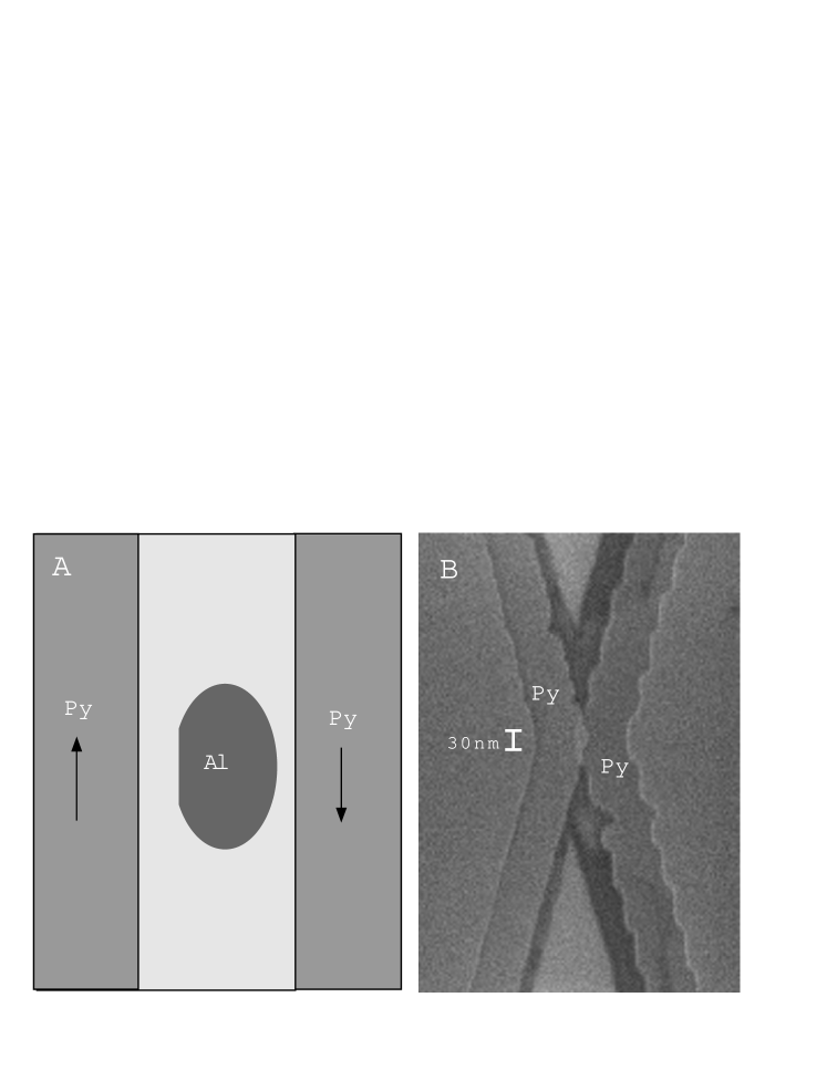
Figure 1: A: Sketch of sample cross-section in the antiparallel magnetization configuration of the leads. B. Scanning Electron micrograph of a typical device. The tunneling junction with embedded nanoparticles is located inside the overlap of two Py leads.

The saturation effect was explained by a rapid increase of the spin-relaxation time with the nanoparticle excitation energy. By this interpretation, the spin-polarized current through the nanoparticle is carried only via the ground state and the few lowest energy excited states of the nanoparticle, while highly excited spin-polarized states relax faster than the average sequential electron tunnel process. We conjectured that at the saturation voltage, the relaxation time of the highest singly occupied energy level of the nanoparticle is comparable to the electron tunnel rate. The corresponding spin relaxation time is in the microsecond range. In comparison, the spin relaxation time in Aluminum thin films with a similar mean free path would be five orders of magnitude shorter.

Our measurement of the spin-relaxation time was somewhat indirect, because theoretical literature prior to our work had not predicted any saturation of the spin-polarized current with bias voltage. Barnas and Fert (1998a); Majumdar and Hershfield (1998); Barnas and Fert (1998b); Brataas et al. (1999a, b); Korotkov and Safarov (1999); Barnas and Fert (1999); Barnas et al. (2000); Imamura et al. (1999); Kuo and Chen (2002); Weymann and Barnas (2003); Brataas and Wang (2001); Wetzels et al. (2006); Weymann et al. (20053); Braun et al. (2005); Urban et al. (2007) Consequently our explanation of the saturation was qualitative. The goal of this paper is to obtain a model of spin-polarized electron transport through a metallic nanoparticle to explain our observations. We use a method for calculating current via energy levels of the nanoparticle based on rate equations, following Ref. Bonet et al. (2002). The tunneling regime in our devices is different from that used in the theoretical studies, because the tunnel resistances in our junctions are highly asymmetric and spin-relaxation rate has strong energy dependence. Barnas and Fert (1998a); Majumdar and Hershfield (1998); Barnas and Fert (1998b); Brataas et al. (1999a, b); Korotkov and Safarov (1999); Barnas and Fert (1999); Barnas et al. (2000); Imamura et al. (1999); Kuo and Chen (2002); Weymann and Barnas (2003); Brataas and Wang (2001); Wetzels et al. (2006); Weymann et al. (20053); Braun et al. (2005); Urban et al. (2007)

Other experimental work on arrays and single nanoparticles did not find any saturation of the spin-polarized current with bias voltage. Yakushiji et al. (2001); Yakushiji2002; Yamane2004; Zhang et al. (2005); Yakushiji2007; Yakushiji2007a; Bernand-Mantel et al. (2006) These experiments do not measure TMR in the regime of well resolved energy levels, we believe that this is a critical measurement to separate the contributions to $TMR$ from the chemical potential shifts. The analysis of $TMR$ experiments in Ref. Seneor et al. (2007) uses an energy independent spin-relaxation time. It is possible, however; that the energy dependence of the spin-relaxation rate can be quite strong. Yafet (1963) We show in this paper that the effect of the energy dependence on spin-polarized current is significant.

Our model is valid within a specific experimental regime, outlined in Sec. IV, but it is an easily analyzable and experimentally relevant regime that merits consideration as a large number of samples fall under this parameter range.

In Sec. II we review the effects of spin-orbit scattering in metallic nanoparticles, in the context of spin-injection and detection. In Sec. III we discuss various energy-relaxation rates in the nanoparticle. The criteria of the model validity are listed on Sec. IV. We then calculate the probability distribution of the many-electron states in the nanoparticle in Sec. V and use this to calculate a TMR versus bias voltage curve that can be fit to experimental data in Sec. VIII

II Effects of spin-orbit interaction on spin-polarized current through a nanoparticle.

In a metallic nanoparticle, the stationary electronic wavefunctions in zero applied magnetic field are two fold degenerate and form Kramers doublets:

$$|\uparrow>^{\prime}=u(\vec{r})|\uparrow>+v(\vec{r})|\downarrow>,$$

$$|\downarrow>^{\prime}=u^{\star}(\vec{r})|\downarrow>-v^{\star}(\vec{r})|\uparrow>.$$

The mixing between the spin-up and the spin-down components is caused by the spin-orbit interaction. In a magnetic field, the degeneracy is lifted by the Zeeman effect. If the field is applied in direction corresponding to $|\uparrow>$, the g-factor is $g=2-4\int d^{3}\vec{r}|v|^{2}<2$.

The effects of the spin-orbit interactions on the wavefunctions are described by a dimensionless parameter $\lambda$

$$\lambda=\sqrt{\frac{\pi\hbar\nu_{SO}}{\delta}},$$ (1)

where $\nu_{SO}$ is the spin-orbit scattering rate and $\delta$ is the average spacing between successive Kramers doublets in the particle. Matveev et al. (2000); Brouwer et al. (2000); Adam et al. (2002) The effects of spin orbit scattering are weak if $\lambda\ll 1$. In that case, $v(\vec{r})\approx 0$, $u(\vec{r})$ is real, and the wavefunctions $|\uparrow>^{\prime}$ and $|\downarrow>^{\prime}$ have well defined spin. In the opposite limit, $\lambda\gg 1$, the spin-orbit scattering is strong. In that case, $\int d^{3}\vec{r}|u|^{2}\approx\int d^{3}\vec{r}|v|^{2}\approx 1/2$ and the wavefunctions have uncertain spin.

Consider an electron with spin-up injected by tunneling from a ferromagnet into the nanoparticle. If the tunnel process is instantaneous, the electron will have a well defined spin $|\uparrow>$ immediately after tunneling. In the regime of weak spin-orbit scattering, where $v\approx 0$, the initial state has a much larger overlap with a wavefunction $|\uparrow>^{\prime}$ than with the corresponding wavefunction $|\downarrow>^{\prime}$. As a result, the spin of the added electron will remain well defined, in principle indefinitely long, barring any coupling between the nanoparticle and the environment. In that case, the detection of the injected spin can be performed at any time after the injection.

By contrast, in the regime of strong spin-orbit scattering, the initial state overlaps with both $|\uparrow>^{\prime}$ and $|\downarrow>^{\prime}$, nearly equally. In that regime, the spin of the added electron becomes uncertain after a time $\sim\tau_{SO}=1/\nu_{SO}$, so there is a time limit $\sim\tau_{SO}$ for spin detection.

In normal metals, there is a scaling between the spin-conserving electron scattering rate and the corresponding spin-flip electron scattering rate, Yafet (1963); Elliot (1954)

$$\nu_{SO}(\omega)=\alpha\nu(\omega).$$ (2)

This is known as the Elliot-Yafet relation. $\omega$ is the energy difference between the initial and final state. For elastic scattering, $\omega=0$ and $\nu_{SO}(0)=\nu_{SO}$. The scaling parameter $\alpha$ depends on the spin-orbit scattering and the band structure. In Aluminum, $\alpha\approx 10^{-4}$ is larger than anticipated from the spin-orbit interaction, because of the hot-spots for spin scattering in the band structure. Fabian and Sarma (1998, 1999)

The Elliot-Yafet relation was confirmed in bulk metals by the conduction-electron spin resonance experiments (CESR). In particular, the temperature dependence of the width of the spin-resonance line, which is proportional to $\nu_{SO}(k_{B}T)$, follows the temperature dependence of the resistivity, which is proportional to the momentum relaxation rate, in agreement with Eq. 2. The relation has also been confirmed more recently in mesoscopic metallic samples, by the spin-injection and detection experiments. Jedema et al. (2001, 2002, 2003) Both CESR and spin-injection and detection experiments measure the time decay of a nonequilibrium spin population in the regime of strong spin-orbit scattering.

In metallic nanoparticles, the validity of the Elliot-Yafet relation was confirmed experimentally by energy level spectroscopy, in the regimes of weak and moderate spin-orbit scattering. Petta and Ralph (2001) $\nu_{SO}$ can be measured directly from the magnetic field dependence of the energy levels. Adam et al. (2002) Petta et al. Petta and Ralph (2001) found that in Cu, Ag, and Au nanoparticles, $\nu_{SO}\approx\alpha v_{F}/D$, where $v_{F}$ is the Fermi velocity and $D$ is the nanoparticle diameter, and $\alpha$ is close to the bulk value, within an order of magnitude. This confirms the Elliot-Yafet relation because $v_{F}/D$ is equal to the elastic scattering rate, assuming a ballistic nanoparticle. More recently, the Elliot-Yafet relation was confirmed in Al nanoparticles as well. Wei et al. (2007)

Substituting the level spacing and the Elliot-Yafet relation into Eq. 1, we find that there is a characteristic nanoparticle size

$$D^{\star}=\lambda_{F}/\sqrt{\alpha}.$$ (3)

Spin-orbit scattering will be weak if $D\ll D^{\star}$ and spin-orbit scattering will be strong if $D\gg D^{\star}$. $D^{\star}$ is a material dependent microscopic parameter. In Aluminum, $D^{\star}\approx 10^{2}\lambda_{F}\sim 10nm$.

It follows that both mesoscopic and macroscopic metallic samples are in the regime of strong spin-orbit scattering. Only if the nanoparticle diameter is less than about 10nm the spin-orbit scattering becomes weak. In samples much larger than $D^{\star}$, measuring the discrete electron energy levels and the electron spin polarization are incompatible, and the spin-polarized current via resolved energy levels must be negligibly small. We are not aware of any theory that explicitly takes into account the effect of spin-mixing in the Kramers doublets on $TMR$ of ferromagnetic single-electron transistors, e.g. that calculates $TMR$ versus $\lambda$. Such a theory would be important because it would set the limits of observability of spin-polarized current through single electron transistors.

In samples much larger than $D^{\star}$, one can still study the time decay of injected electron spins at a time scale much shorter than the time necessary to resolve discrete energy levels (the Heisenberg time $\hbar/\delta$), as demonstrated by the CESR experiments and spin-injection and detection in mesoscopic metals. In further discussion, we assume $D\ll D^{\star}$. In that case, the spin up band in the ferromagnet is tunnel coupled to the nanoparticle wavefunctions with spin-up only.

III Energy Relaxation in Metallic Nanoparticles

In this work we study spin-polarized electron current via discrete energy levels of metallic nanoparticles, in a regime where the tunnel rate is much smaller than the spin-conserving energy relaxation rate. The tunnel rate can still be larger than the spin-flip relaxation rate, so electrons in the nanoparticle are not in equilibrium.

Consider a nanoparticle with an electron added at energy $\omega=\delta$, as shown in Fig. 2. The nanoparticle is in an excited state and it can relax its energy internally. It was shown that the dominant relaxation process is electron-phonon interaction. Agam et al. (1997) One possible path for this relaxation is spin-conserving, as shown in Fig. 2-A. The spin-conserving relaxation rate via phonon emission have been estimated by Agam et al. Agam et al. (1997)

$${\nu_{e-ph}(\omega)}=\left(\frac{2}{3}E_{F}\right)^{2}\frac{\omega^{3}\tau_{e}\delta}{2\rho\hbar^{5}v_{s}^{5}},$$ (4)

where $E_{F}=11.7eV$ is the Fermi energy, $\omega$ is the energy difference between the initial and the final state, $\tau_{e}$ is the elastic scattering relaxation time, $\rho=2.7g/cm^{3}$ is the ion-mass density, and $v_{s}=6420m/s$ is the sound velocity. This formula is equivalent to

$$\hbar\nu_{e-ph}(\omega)\sim\frac{1}{g}E_{F}\left(\frac{\omega}{\omega_{D}}\right)^{3},$$

within a prefactor of order 1, where $\omega_{D}$ is the Debye energy and $g$ is the dimensionless conductance of the nanoparticle, $g=E_{Th}/\delta$, and $E_{Th}=\hbar v_{F}/D$ is the Thouless energy. This relation is similar to the formula for bulk electron-phonon scattering rate, except that there is a prefactor $1/g$, Agam et al. (1997) which originates from the chaotic nature of the electron wavefunctions.

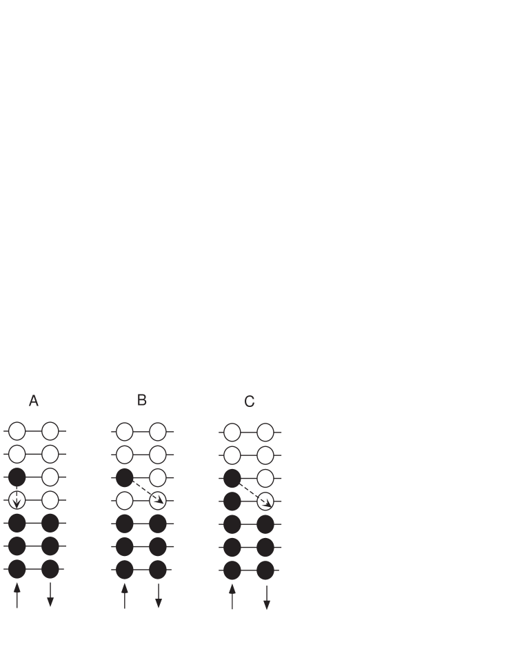
Figure 2: A: Spin-conserving energy relaxation process. B. Spin-flip energy relaxation process. C: Electronic state with the relaxation time equal to the spin-flip relaxation time. 

We estimate $\nu_{e-ph}(\delta)\sim GHz$ in nanoparticle with diameter $5nm$, in agreement with experiment. Ralph et al. (1995) All our samples have tunnel rates significantly smaller than this relaxation rate, so, the nanoparticle can be considered to be relaxed toward the lowest energy state accessible via spin-conserving transitions.

The nanoparticle can also relax through a transition depicted in Fig. 2-B, with some rate $\nu^{SF}(\omega)$, $\omega=\delta$. This spin-flip transition involves coupling between electrons and the environment, which may be the phonon bath or the bath of nuclear spins. In zero applied magnetic field, the electron transitions shown in Figs. 2-A and B have the same energy difference between the initial and the final states. We expect that the transition rate for the spin-flip relaxation process is much smaller than the corresponding spin-conserving relaxation rate, because in the spin-flip process there must be a transfer of angular momentum into the environment.

For example, if the environment is the ion lattice, then the transfer is governed by the spin-orbit interaction, which is much smaller than the the electrostatic interaction that governs the spin-conserving transitions. Thus the spin-flip probability caused by the spin-orbit interaction during a phonon emission process is very small. It is reasonable to expect that the Elliot-Yafet scaling is valid for the transitions between chaotic wavefunctions, so that $\nu^{SF}(\omega)=\alpha\nu_{e-ph}(\omega)$, but we are not aware of any theoretical calculation of the spin relaxation rate in metallic nanoparticles.

Spin-flip electron transition rates between discrete levels were obtained theoretically for semiconducting quantum dots. Khaetskii and Nazarov (2000, 2001) The theoretical calculations were in good agreement with the experimental results in GaAs quantum dots. Hanson et al. (2003) The theory of spin-relaxation in semiconducting quantum dots is of no use for metallic nanoparticles, because the mechanisms of spin-orbit interaction in metals and semiconductors are very different. Zutic2004

It would be very difficult to measure the transition rate depicted in Fig. 2-B, because the relaxation process in Fig. 2-A competes with that in Fig. 2-B. We are able to determine the spin relaxation rates in tunneling measurements because it is possible to trap the nanoparticle into a state shown in Fig. 2-C. In that case the spin-conserving energy relaxation is forbidden by the Pauli principle and the relaxation rate is equal to the spin relaxation rate.

IV Region of model validity

In this paper the tunnel current via discrete energy levels of a metallic nanoparticle is calculated using the methods outlined in Ref. Bonet et al. (2002) We consider spin polarized tunneling in the regime closest to our experiments. The following conditions define that regime.

1. We assume that the tunnel junctions in our samples are highly asymmetric in resistance. The asymmetry arises because the tunnel junctions are fabricated using conventional lithography and evaporation. A weak non-uniformity in the tunnel junction thickness leads to large asymmetry in the tunnel resistance. Wei et al. (2007)

In these asymmetric samples, the current through the nanoparticle is limited by the tunnel rate through the high resistance junction. The resistance of the low resistance junctions is less directly related to the current and it can be obtained by comparing the amplitudes of Zeeman split energy levels at positive and negative bias voltage. That procedure has been described in detail in some special cases in Ref. Bonet et al. (2002) Even though our regime is quite different from those special cases, they are still indicative of the procedure to determine the resistance ratio. Applying the general formalism of Ref. Bonet et al. (2002) to our regime we estimate the resistance ratio to be about 25 in sample 1. The results of our model do not depend on the resistance ratio, as long as the electron discharge rate is much larger than the electron tunnel in rate.

2. We calculate the current in the regime when the first tunnel step is across the high resistance junction. This step is followed by an electron discharge via the low-resistance junction. This regime is relatively easy to analyze because electron discharge is fast and so the charging effects do not influence the current significantly. Averin et al. (1999); Bonet et al. (2002) In this case, the nanoparticle spends most of the time waiting for an electron to tunnel in.

3. We assume $E_{C}\gg\delta$, where $E_{C}$ is the charging energy. This assumption is generally valid in metallic nanoparticles. Ralph et al. (1995)

4. We assume that the coulomb gap in the I-V curve is much larger than the level spacing, this requires not only that condition 3 is met, but that the background charge $q_{0}$ is not too close to $(n+1/2)e$, where $n$ is an integer. In that case the number of energy levels participating in electron transport is always $\gg 1$. Even if an electron tunnels into the lowest unoccupied single-electron energy level of the nanoparticle, there will still be a large number of occupied single-electron energy levels of the nanoparticle that can discharge an electron.

5. We assume that the number of electrons on the nanoparticle before tunneling in is even. The calculation for the odd case is very similar to that for the even case and will not be discussed here.

6. We assume that the tunnel rates between the single-electron states $i$ in the nanoparticle and the leads are much smaller than the spin-conserving energy relaxation rates, which are $>GHz$. In the sample selected for this paper, the tunnel rate across the high resistance junction is in the $MHz$ range.
If the spin-relaxation process is taking place and there is a large asymmetry in junction resistances, an important question is which one of the two tunnel rates limits the $TMR$. We will assume that the left junction has higher resistance. It may be tempting to assume that $TMR$ will be highly asymmetric with bias voltage if $\Gamma^{L}\ll\nu^{SF}(\omega)\ll\Gamma^{R}$, where $\Gamma^{L}$ and $\Gamma^{R}$ are the electron tunnel rates between the energy levels of the nanoparticle and the left and the right leads, respectively, because, if a spin-polarized electron tunnels in via the high resistance junction, it will tunnel out via the low resistance junction before spin-relaxation process takes place, and, if the direction of the current is reversed, the order of tunneling will be reversed and the spin-relaxation will take place before tunneling out. A similar situation is found in measurements of the energy spectra in samples where $\Gamma^{L}\ll\nu_{e-ph}(\omega)\ll\Gamma^{R}$, where $\nu_{e-ph}(\omega)$ is the spin-conserving energy relaxation rate. In that case, electron transport is much closer to equilibrium in one direction of current than in another direction of the current, resulting in asymmetric energy level spectra. Ralph et al. (1995)
It turns out that in spin injection and detection in the regime defined in this section, $TMR$ is symmetric even if $\Gamma^{L}\ll\nu^{SF}(\omega)\ll\Gamma^{R}$. The reason is that the spin-polarized current is mediated by spin-accumulation, which takes place after a large number of tunnel-in and tunnel-out steps.
Assume that an electron first tunnels in via the low resistance junction and then an electron tunnels out via the high resistance junction. In that case, it is clear that in order to observe spin polarized current, it is necessary that the spin-relaxation time in the nanoparticle be longer than the tunnel out time.
If the bias voltage is reversed, an electron first tunnels in via the high resistance junction and then an electron tunnels out via the low resistance junction. In our regime, it is highly improbable that the same electron tunnels in and out, because the number of occupied electron states available for discharge is $\gg 1$. To obtain a spin-polarized current in this case, the spin-accumulation in the nanoparticle is necessary, which takes place after many tunnel in and tunnel out steps and makes it necessary that the spin of the nanoparticle be conserved during the time that the nanoparticle waits before an electron tunnels in. Overall, the spin-polarized current and $TMR$ are comparable in magnitude for the two current directions, in agreement with our measurements.

V Calculation of the Spin Probability Distribution in the Nanoparticle

In this section we obtain the probability distribution among various many-electron states $|\alpha>$ generated by electron tunneling via the nanoparticle. The many-electron states are the Slater determinants of varying single-electron states of the nanoparticle. In further discussion, the many electron states will be referred to simply as states.

The number of electrons and the total spin can vary among the states. The time dependence of the occupational probability $Q_{\alpha}$ is given by the masters equation, Averin et al. (1999); Beenakker (1991)

$$\frac{dQ_{\alpha}}{dt}=\sum_{{\beta}\neq\alpha}\left(\Gamma_{{\beta}\to{\alpha}}Q_{\beta}-\Gamma_{{\alpha}\to{\beta}}Q_{\alpha}\right),$$ (5)

where $\Gamma_{{\alpha}\to{\beta}}$ is the transition rate from state $|\alpha>$ to state $|\beta>$.

The steady state solutions are obtained from the masters equation using $\frac{dQ_{\alpha}}{dt}=0$. The masters equations then mutually relate the occupational probabilities of various states. In addition, the occupational probabilities are normalized, that is, the sum of all occupational probabilities is equal to one. The masters equation in the steady state and the normalization condition are sufficient to determine the occupational probabilities. The current through the left barrier is obtained as

$$I_{L}=|e|\sum_{\alpha}\sum_{\beta}\Gamma_{\alpha\to\beta}^{L}Q_{\alpha},$$ (6)

where $\Gamma_{\alpha\to\beta}^{L}$ is the contribution of the left lead to the transition rate $\Gamma_{\alpha\to\beta}$, taken with a positive or negative sign depending on weather the transition gives a positive or negative contribution to the current, respectively. Averin et al. (1999); Beenakker (1991); Bonet et al. (2002)

Because the tunnel density of states in the ferromagnets is spin-dependent, $Q_{\alpha}$ will depend on the relative magnetic orientations of the leads. We set the magnetization of the left ferromagnetic lead to be always up. The magnetization of the right ferromagnetic lead can be up or down, corresponding to values of parameter $\sigma$: if $\sigma=1$ the magnetizations are parallel and if $\sigma=-1$ the magnetizations are antiparallel.

The tunnel-densities of states at the Fermi level of spin up and spin down electrons in the left lead are $N_{\uparrow}=N_{av}(1+P)$ and $N_{\downarrow}=N_{av}(1-P)$, respectively, where $N_{av}$ is the average tunnel-density of states at the Fermi level per spin band, and $P$ is the spin-polarization of the ferromagnet. Similarly, the tunnel densities of states at the Fermi level in the right lead are $N_{\uparrow}=N_{av}(1+\sigma P)$ and $N_{\downarrow}=N_{av}(1-\sigma P)$ for spin-up and spin-down electrons, respectively.

We assume that electron spin is conserved in the tunnel process across a single tunnel junction. This assumption is justified by the fact that samples without nanoparticles have a large and weakly voltage dependent $TMR$. Wei et al. (2007) In that case, the spin-up (down) bands in the leads are tunnel-coupled only to the discrete levels in the nanoparticle with spin up (down). This is also valid because the single-electron states in the nanoparticle have well defined spin, since the spin-orbit coupling in the nanoparticle is weak, as discussed earlier.

The tunnel rate between the leads and a discrete level $i$ is proportional to the tunnel-density of states in the leads and can be written as $\Gamma_{i}(1+P)$ for spin-up electrons and $\Gamma_{i}(1-P)$ for spin-down electrons, where $\Gamma_{i}$ is referred to here as the bare tunnel rate.

Next we use the masters equation to obtain the current in the regime defined in Sec. IV. To summarize, at zero bias voltage the number of electrons on the nanoparticle is even. We investigate the region of the IV-curve where only one extra electron can be added to the nanoparticle, within the first step of the Coulomb-staircase. This is the bias-voltage region where the saturation of the spin-polarized current with bias voltage is observed. We consider highly asymmetric junctions in resistance, $R_{L}\gg R_{R}$. A positive bias voltage is applied on lead $R$ relative to lead $L$, so first an electron tunnels into the nanoparticle from the left lead, across the high-resistance junction, and after that the nanoparticle discharges one electron into the right lead via the low resistance junction. Finally, the internal spin-conserving relaxation rates are much larger than both tunnel rates, $\nu(\omega)\gg\Gamma^{R}\gg\Gamma^{L}$.

In this regime, it is convenient to divide the states into four groups. Group 1 contains the states which do not have an added electron and which are fully relaxed with respect to spin-conserving transitions. We describe these states in detail before discussing other groups.

Consider the states which do not have an added extra electron displayed in Fig. 3. The internal relaxation of the states in the figure must involve a spin-flip process. So the states are fully relaxed with respect to spin-conserving transitions, thus they are in group 1. In the figure, the charging energy has been added to the single-electron energy levels of the nanoparticle, to make it clear which unoccupied single-electron energy levels are accessible for tunneling in from the left lead. As seen in the figure, the states from group 1 can be labelled $|i>$, where $i=-N,-N+1,...,N-1,N$, where $N=4$ for the example shown in the figure.

$N$ is the number of unoccupied single-electron states above the Fermi level of the nanoparticle into which an electron can tunnel in from the left lead. It is related to the bias voltage. If the level spacing $\delta$ is constant, then $N=e\frac{C_{R}}{C_{L}+C_{R}}(V-V_{CB})/\delta$, Wei et al. (2007) where $C_{L}$ and $C_{R}$ are the capacitances of the left and the right tunnel junction, respectively, and $V_{CB}$ is the Coulomb blockade threshold voltage. 

$N$, the number of single-electron states that are accessible for tunneling-in, is different from the number of single-electron states that can discharge an electron ($M$). For example, if the nanoparticle is in state $|0>$, then an electron from the left lead can tunnel only into one of the unoccupied single-electron levels labelled $1,2,...,N$ with either spin. After an electron tunnels in, the nanoparticle can discharge either the added electron or any other spin-up or spin-down electron from one of the doubly occupied single-electron states labelled $0,-1,-2,...,-M$ ($M=12$ in the figure), consistent with Coulomb blockade. Averin et al. (1999); Beenakker (1991) If the level spacing is constant, then $M=eV_{CB}/\delta$.

Group 2 contains states which do not have an added electron and which can internally relax by spin-conserving transitions. Group 3 contains states with an added extra electron and which are fully relaxed with respect to spin-conserving transitions. Finally, group 4 contains the states with an added extra electron and which can internally relax by spin-conserving transitions.

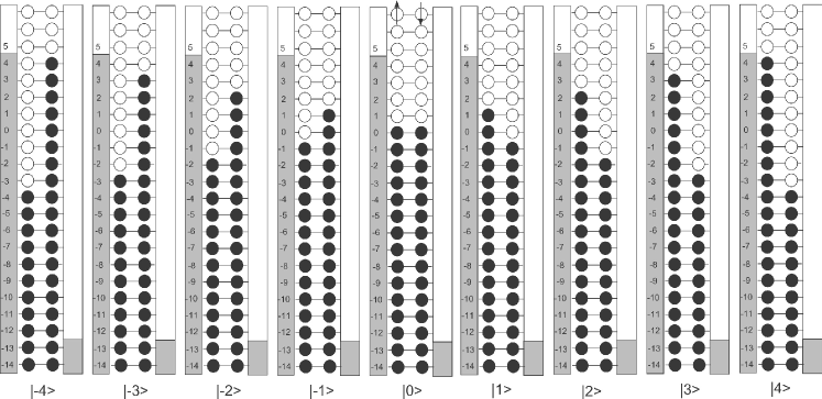
Figure 3: Many-electron states from group 1. Black-filled and white-filled circles indicate occupied and unoccupied single-electron states, respectively. Only one electron can tunnel into the nanoparticle at a time because of the Coulomb Blockade; the displayed states are found before an electron tunnels into the nanoparticle from the left lead and after an electron tunnelled out of the nanoparticle into the right lead. The states are fully relaxed with respect to internal spin-conserving transitions.  

The next task is to determine the steady state occupational probabilities. Using $\nu(\omega)\gg\Gamma^{R}\gg\max(\Gamma^{L},\nu^{SF}(\omega))$, several approximations can be made in the masters equation.

First, it is shown in the appendix that the occupational probabilities $Q_{i}$ of the states from the first group are larger than the occupational probabilities of the states from the second, third, and the forth group, by a factor of $\frac{\nu(\omega)}{\Gamma^{L}}$,$\frac{\Gamma^{R}}{\Gamma^{L}}$, and $\frac{\nu(\omega)}{\Gamma^{L}}$, respectively. The occupational probabilities of the states from groups 2-4 can thus be neglected in the normalization condition, so

$$\sum_{i=-N}^{N}Q_{i}=1,$$

with an error of order $\frac{\Gamma^{L}}{\Gamma^{R}}\ll 1$, in the limit $\nu(\omega)\gg\Gamma^{R}\gg\Gamma^{L}(\omega)$.

Second, if $\nu(\omega)\gg\Gamma^{R}\gg\max(\Gamma^{L},\nu^{SF}(\omega))$, the occupational probabilities of the states from the second, third, and the forth group of states can be eliminated from the masters equations in an explicit way. The elimination leads to a set of linear equations that relate the occupational probabilities within the space of states $G_{1}$. These equations are refereed to here as the renormalized masters equation:

$$Q_{i}\sum_{m\neq i}\Gamma_{i\to m}^{ren}=\sum_{m\neq i}Q_{m}\Gamma_{m\to i}^{ren},$$ (7)

where $\Gamma_{m\to i}^{ren}$ is the renormalized transfer rate from state $|m>$ to state $|i>$.

The transfer $|m>\to|i>$ takes place either directly, via a spin-flip transition, or indirectly via intermediate states. In the leading order of $\frac{\Gamma^{L}}{\nu(\omega)}$,$\frac{\Gamma^{L}}{\Gamma^{R}}$, $\Gamma_{m\to i}^{ren}$ is equal to $\Gamma_{m\to i}$ (direct transition rate from $m$ to $i$) plus the sum of the rates of transitions from state $|m>$ into the intermediate states, weighted by the probability of transfer from the intermediate states into the state $|i>$:

$$\Gamma_{m\to i}^{ren}=\Gamma_{m\to i}+\sum_{\alpha}\Gamma_{m\to\alpha}\Pi(\alpha\to i),$$ (8)

$\Pi(\alpha\to i)$ is the probability that the nanoparticle in intermediate state $|\alpha>$ will transfer into state $|i>$.

In the following, we will obtain $\Gamma_{i\to m}^{ren}$ in an intuitive way. This approach emphasizes understanding and enables one to obtain the occupational probabilities $Q_{i}$ from the renormalized masters equation directly, without explicitly solving the masters equation. In the appendix, we will derive $\Gamma_{m\to i}^{ren}$ from the masters equation and show that the intuitive approach is accurate within controlled approximations.

VI Nanoparticle Spin Probability Distribution in Absence of Spin-Relaxation

In this section we examine the regime where no spin-relaxation takes place, $\nu(\omega)\gg\Gamma^{R}\gg\Gamma^{L}\gg\nu^{SF}(\omega)$. In that case, all transfers between the states within the space of states $|i>$ are indirect. They involve a sequential electron tunneling process, in which the nanoparticle goes into an intermediate state with an extra added electron. $\Gamma_{m\to i}^{ren}$ is equal to the sum of the rates of transitions from state $|m>$ into the various intermediate states with an added extra electron, weighted by the probability of transfer from these intermediate states into the state $|i>$.

Consider the nanoparticle in state $|i>$, which has spin $i\hbar$, ($i>1$). After an electron tunnels into the nanoparticle, the nanoparticle is in an intermediate state with spin $(i+1/2)\hbar$ or $(i-1/2)\hbar$. Then, after an electron tunnels out, the nanoparticle spin changes again by $\hbar/2$ or $-\hbar/2$, so the final spin after a sequential tunneling process can be $(i-1)\hbar$, $i\hbar$, and $(i+1)\hbar$. So the renormalized transfer rate from state $|i>$ into states $|m>$ is nonzero only if $m=i-1$ or $m=i$ or $m=i+1$.

The nanoparticle will transfer from state $|i>$ to state $|i+1>$ indirectly, if a spin-up electron tunnels in from the left lead and then a spin-down electron tunnels out into the right lead. A spin-up electron can tunnel into any of the unoccupied single-electron states $k$ with spin-up, $k=i+1,i+2,...N$. After tunneling in, the nanoparticle instantly relaxes via spin-conserving transition. A spin-down electron can then tunnel out from any of the occupied single-electron states $j$ with spin down, $j=-M,-M+1,...,-i$. Then, if the nanoparticle after tunneling out is left in an excited state, it will relax instantly into state $|i+1>$.

The rate for this spin-up-tunnel-in / spin-down-tunnel-out sequential process is obtained from Eq. 8, by summing over all the intermediate states with an added extra electron,

$$\Gamma_{i\to i+1}^{ren}=\sum_{k=i+1}^{N}\Gamma_{k}(1+P)\pi_{i}(\downarrow)$$ (9)

where $\pi_{i}(\downarrow)$ is the probability that the nanoparticle with an added spin-up electron will discharge a spin-down electron.

The rate at which a spin-down electron discharges is $\sum_{j=-M}^{-i}\Gamma_{j}^{R}(1-\sigma P)$, where $\Gamma_{j}^{R}$ is the bare tunnel rate between level $j$ and the right lead. Similarly, the rate at which a spin-up electron discharges is $\sum_{j=-M}^{i+1}\Gamma_{j}^{R}(1+\sigma P)$. The probabilities $\pi_{i}(\uparrow)$ and $\pi_{i}(\downarrow)$ are proportional to the spin-up and spin-down discharge rates, respectively. The total discharge probability is one, $\pi_{i}(\uparrow)+\pi_{i}(\downarrow)=1$, so we obtain

$$\pi_{i}(\downarrow)=\frac{(1-\sigma P)/2}{1+\frac{(1+\sigma P)\sum_{j=-i+1}^{i+1}\Gamma_{j}^{R}}{2\sum_{j=-M}^{-i}\Gamma_{j}^{R}}}$$ (10)

As discussed previously, in our model the number of discharging levels $M\gg 1$. We make a further assumption that $M\gg N$, which is valid not too far from the conduction threshold for sequential electron tunneling through the nanoparticle. In this case, the denominator in Eq. 10 is close to one, within a factor of $i/M\sim N/M$, and we obtain

$$\pi_{i}(\downarrow)=\frac{1-\sigma P}{2},\pi_{i}(\uparrow)=\frac{1+\sigma P}{2}.$$

The approximation $N/M\ll 1$ enhances the probability to discharge a spin-down electron at the expense of suppressing the probability to discharge a spin-up electron. So the approximation increases the spin accumulation efficiency. This approximation is not essential for our model to work, but it simplifies further calculations.

Substituting into Eq. 9, we obtain

$$\Gamma_{i\to i+1}^{ren}=A_{i+1}(P),$$ (11)

where

$$A_{i}(P)=\frac{(1+P)(1-\sigma P)}{2}\sum_{j=i}^{N}\Gamma_{i}.$$ (12)

Now we consider the indirect transfer $|i>\to|i-1>$. In this transfer process, an electron with spin-down tunnels in from the left lead, followed by a discharge of an electron with spin-up into the right lead. Following an analysis similar to the above, we find $\Gamma_{i\to i-1}^{ren}=A_{-i+1}(-P)$. The left hand side of Eq. 7 becomes $Q_{i}(A_{i+1}(P)+A_{-i+1}(-P))$. Using Eqs. 11 and  26, the steady state Eq. 7 becomes

$$Q_{i}(A_{i+1}(P)+A_{-i+1}(-P))$$

$$=$$ Q_i-1A_i(P)+Q_i+1A_-i(-P), (13)

where $i=1,2,...N$. At $i=N$, in Eq. 13 we must put $A_{N+1}(P)=0$ and $Q_{N+1}=0$.

A similar analysis to the above leads to a steady state equation for the states with negative nanoparticle spin $|-i>$, $i=1,2,...,N$:

$$Q_{-i}(A_{i+1}(-P)+A_{-i+1}(P)$$

$$=$$ Q_-i+1A_i(-P)+Q_-i-1A_-i(P), (14)

where $i=1,2,...N$. At $i=N$, in Eq. 14 we must put $A_{N+1}(-P)=0$ and $Q_{-N-1}=0$. The final equation necessary for finding $Q_{i}$ is $\sum_{i=-N}^{N}Q_{i}=1$.

We calculate the probability distribution numerically for arbitrary $N$, $\Gamma_{i}$, and $\Omega_{i}$, allowing for fluctuations among different tunnel rates $\Gamma_{i}$ across the left tunnel junction. Once the probability distribution is determined, the current though the nanoparticle is calculated from Eq. 6, which can be shown to be:

$$\frac{I}{|e|}=$$ ∑_ i=-N^NQ_iIi—e— = Q_0∑_j=1^N2Γ_j+ (15)

$$\quad\sum_{i=1}^{N}Q_{i}\left(\sum_{j=i+1}^{N}2\Gamma_{j}+\sum_{j=-i+1}^{i}\Gamma_{j}(1-P)\right)+$$

$$\quad\sum_{i=1}^{N}Q_{-i}\left(\sum_{j=i+1}^{N}2\Gamma_{j}+\sum_{j=-i+1}^{i}\Gamma_{j}(1+P)\right)$$

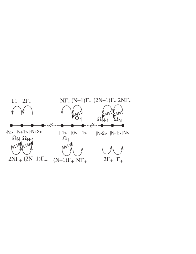
Figure 4: Rates of tunnel and internal relaxation transitions between nanoparticle states $|i>$ in Fig. 3, for the antiparallel magnetic orientations. For simplicity, the bare tunnel rates to the left lead ($\Gamma_{k}=\Gamma$) are assumed to be independent of single-electron energy levels $k$. $\Gamma_{+}=\Gamma(1+P)^{2}/2$, and $\Gamma_{-}=\Gamma(1-P)^{2}/2$. In the parallel magnetization configuration, substitute $\Gamma_{+}$ and $\Gamma_{-}$ with $\Gamma^{\prime}=\Gamma(1-P^{2})/2$. The wavy line indicates spin-relaxation processes. 

To illustrate these equations, we plot the nanoparticle states along an axes, as shown in figure 4. We indicate various transition rates obtained from Eqs. 11 and  26. For simplicity we assume that all bare tunnel-in rates are the same ($\Gamma_{i}=\Gamma$). In that case

$$\Gamma_{i\to i+1}^{ren}=(N-i)\frac{(1+P)(1-\sigma P)}{2}\Gamma,$$ (16)

and

$$\Gamma_{i\to i-1}^{ren}=(N+i)\frac{(1-P)(1+\sigma P)}{2}\Gamma.$$ (17)

The renormalized master equation is

$$Q_{i}\left[(N-i)\Gamma(1+P)(1-\sigma P)/2+(N+i)\Gamma(1-P)(1+\sigma P)/2\right]$$

$$=$$ Q_i-1(N-i+1)Γ(1+P)(1-σP)/2+ (18)

$$Q_{i+1}\left((N+i+1)\Gamma(1-P)(1+\sigma P)/2\right),$$

and the current through the nanoparticle, from Eq. 15, becomes

$$I=|e|\left(2N\Gamma-2<i>P\Gamma\right),$$ (19)

where $<i>=\sum_{i=-N}^{N}iQ_{i}$.

One notices from Fig. 4 that the renormalized rate of transition $|i>\to|i+1>$ decreases as $N-i$, when $i$ increases from zero to N. Similarly, the renormalized rate of transition $|i>\to|i-1>$ increases as $N+i$, when $i$ increases from zero to N. So, if $i$ is near $N$, the rate of $|i>\to|i-1>$ is much larger than the rate of $|i>\to|i+1>$ and in the steady state, $Q_{i}$ must be a rapidly decreasing function of $i$ when $i$ is near $N$. Similarly, $Q_{-i}$ must be rapidly decreasing with $i$ when $i$ approaches $N$.
In the parallel magnetization orientation ($\sigma=1$) the transition rates are symmetric around $i=0$, as explained in Fig. 4. In that case $Q_{i}$ has a maximum at $i=0$, indicating that there is no spin-accumulation in the nanoparticle. This is a situation similar to spin-accumulation in large systems.
In the antiparallel configuration of the leads, the rate of transition $|i>\to|i+1>$ is proportional to $(1+P)^{2}$ and the the rate of transition $|i>\to|i-1>$ is proportional to $(1-P)^{2}$. In that case, transition rate $|i>\to|i+1>$ is larger than transition rate $|i+1>\to|i>$ when $i$ is close to zero, leading to spin-accumulation in the steady state. The spin accumulation is limited because the rate of transition $|i>\to|i+1>$ decreases in proportion with $N-i$ and the rate of transition $|i>\to|i-1>$ increases in proportion with $N+i$, as discussed above.

In the following two sections we focus on limit $N\gg 1$, where we find the analytical solution of $Q_{i}$ and $I$. In the analytic solution we assume that the tunnel rates $\Gamma_{i}$ across the left tunnel junction are independent of $i$, $\Gamma_{i}=\Gamma$.

VI.1 Spin-polarized current at large bias, $N\gg 1$

At the maximum of $Q_{i}$ (the mode), which is found at $i=i_{0}$, the following condition is satisfied: $\Gamma_{i_{0}+1\to i_{0}}^{ren}=\Gamma_{i_{0}-1\to i_{0}}^{ren}$. This leads to

$$i_{0}=\frac{2PN}{1+P^{2}},$$ (20)

in leading order of $N$ in the antiparallel magnetic configuration ($\sigma=-1$). Thus, in the most probable state of the nanoparticle, the chemical potential of spin-up electrons is shifted up by $2i_{0}\delta$ relative to the chemical potential of spin-down electrons,

$$\Delta\mu=\frac{4PN\delta}{1+P^{2}}.$$ (21)

Next we obtain the fluctuations around the mode. We make a conjecture that the probability distribution $Q_{i}$ is sharply peaked around the maximum at $i=i_{0}$, so that the fluctuations around $i_{0}$ are weak compared to $N$. Our numerical calculations show that $rms(i)\sim\sqrt{N}$, confirming the conjecture. We can write $i=i_{0}+j$ and expand $Q_{i}$ around $i=i_{0}$: $Q_{i}=Q+Q^{\prime}j+Q^{\prime\prime}j^{2}/2+...$ . Substituting into Eq. 18, we obtain a differential equation, in leading order of $\sqrt{N}$,

$$\frac{N}{2}\left(\frac{1-P^{2}}{1+P^{2}}\right)^{2}\frac{d^{2}Q}{dj^{2}}+j\frac{dQ}{dj}+Q=0.$$ (22)

This linear differential equation can be solved analytically. Using a boundary condition $Q(\pm N)\ll 1$, the normalized solution is

$$Q_{i}\approx\frac{1+P^{2}}{(1-P^{2})\sqrt{\pi N}}\exp{\left(-\frac{(i-i_{0})^{2}}{N\left(\frac{1-P^{2}}{1+P^{2}}\right)^{2}}\right)},$$ (23)

which is a Gaussian distribution with fluctuation

$$rms(i)=\sqrt{\frac{N}{2}}\frac{1-P^{2}}{1+P^{2}}.$$

A similar analysis leads to the probability distribution in the parallel magnetic configuration:

$$Q_{i}=\frac{1}{\sqrt{\pi N}}\exp{\left(-\frac{i^{2}}{N}\right)},$$ (24)

and $I_{\uparrow\uparrow}=|e|2N\Gamma$, from Eq. 19.

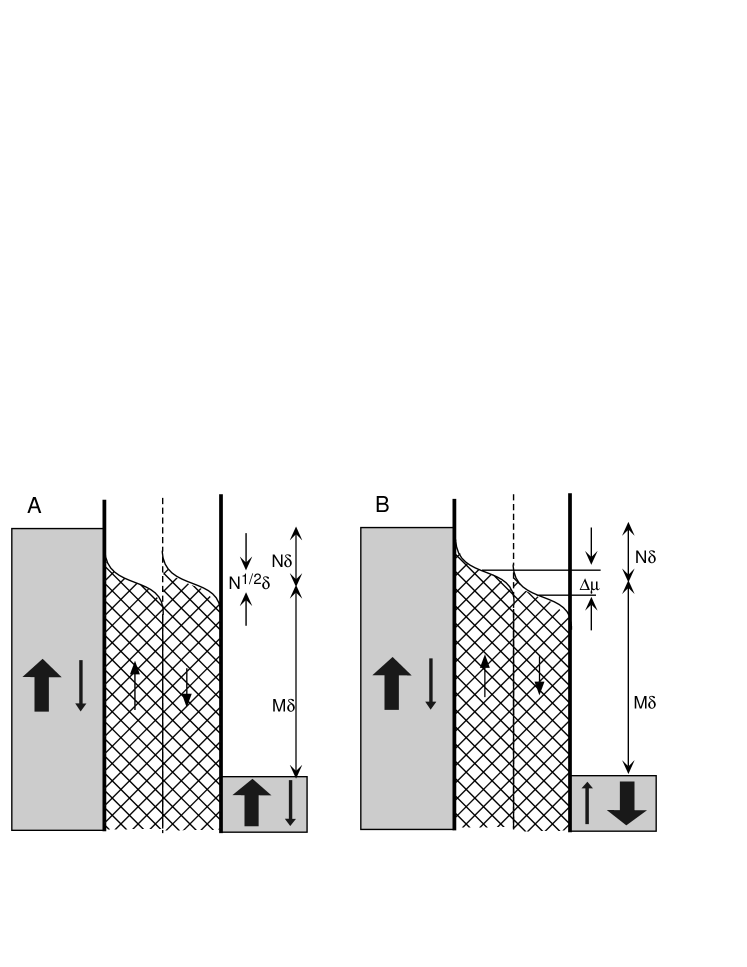
Figure 5: A and B: Probability distribution of electrons in parallel and antiparallel magnetization configuration, when the number of levels $N$ and $M$ are large. 

Fig. 5 displays the electron distribution function in the nanoparticle in the parallel and antiparallel magnetization configurations. The difference in chemical potentials of spin-up and spin-down electrons in the antiparallel state is proportional to $N$, the number of energy levels available for tunneling-in, according to Eq. 21.

Spin accumulation in the nanoparticle is well defined if the relative fluctuation,

$$rms(i)/i_{0}=\frac{1-P^{2}}{2P\sqrt{2N}},$$

is smaller than 1. For example, if $P=0.1$, $N$ must be $>12$ in order to have a well defined spin accumulation. If $N<12$, the time dependence of the nanoparticle spin will exhibit significant noise. In large systems where the level spacing is negligibly small, $N$ is typically $\gg 1$ and the fluctuations are thus negligible.

Using Eq. 19 and the results of this section, the tunnel magnetoresistance can be shown to be

$$TMR=\frac{P<i>}{N}=\frac{2P^{2}}{1+P^{2}},$$ (25)

which is the Jullieres’s formula. Julliere (1975) The Julliere’s value is larger than the $TMR$ predicted theoretically. Weymann et al. (20053) But this theory is valid in a different regime than ours and our approximation slightly enhances the spin-accumulation efficiency, as discussed earlier. Another recent numerical calculation hwang in a regime similar to our own, and an assumption of infinite spin lifetimes confirms the Julliere value as a maximum of the $TMR$ in a nanoparticle.

VII Nanoparticle Spin Probability Distribution with Spin-Relaxation

If spin-relaxation rate is not negligible, then the nanoparticle in state $|i>$ can undergo a spin-flip transition into state $|i-1>$. The nanoparticle spin changes by $\hbar$ in a spin-flip transition, hence there are no other final states in the space of states $G_{1}$ after a spin-flip transition. The renormalized transfer rate is

$$\Gamma_{i\to i-1}^{ren}=A_{-i+1}(-P)+\Omega_{i},$$ (26)

where $\Omega_{i}$ is the total transfer rate from $|i>$ to $|i-1>$ that includes an internal spin flip transition. This transfer can take place directly or via intermediate states. Starting from a state $|i>$ in Fig. 3, an electron occupying the highest single-electron energy level $i$ with spin up can make a transition into the lowest unoccupied single-electron energy level $-i+1$ with spin down. In this process the energy difference is $(2i-1)\delta$ and the rate is $\nu^{SF}[(2i-1)\delta]$. This is a direct transition.

Alternatively, starting from the same sate $|i>$, an electron occupying the highest single-electron energy level $i$ with spin-up can make a transition into the next-to-the lowest unoccupied single-electron energy level $-i+2$ with spin-down. The nanoparticle is left in an excited state, which is an intermediate state. This is followed by a spin-conserving relaxation transition, which is instantaneous in our model, and the nanoparticle ends in the state $|i-1>$. Similarly, starting from state $|i>$, an electron occupying the next-to-the highest single-electron energy level $i-1$ with spin-up can make a transition into the lowest unoccupied single-electron energy level $-i+1$ with spin-down, leaving a hole. This is followed again by an instantaneous spin-conserving relaxation transition, which brings the nanoparticle into the state $|i-1>$. The energy differences for the spin-flip processes are the same, $(2i-2)\delta$, assuming equal level spacing. The total spin-flip transition rate with this energy difference is $2\nu_{SF}[(2i-2)\delta]$.

Taking into account all spin-flip processes with varying energy differences, we find the spin-relaxation rate

$$\Omega_{i}=\sum_{j=0}^{2i-1}(j+1)\nu_{SF}[(2i-j-1)\delta].$$ (27)

In general, we expect $\nu^{SF}(\omega)$ to be rapidly increasing with $\omega$: $\nu^{SF}(\omega)\sim\omega^{n}$. In that case $\Omega_{i}$ increases with energy faster than $\nu^{SF}(\omega)$: $\Omega_{i}\sim i^{n+2}$.

In this analysis we neglect higher order spin-flip transitions $|i>\to|i-2>$, $|i>\to|i-3>$,… , where the environment would receive angular momentum $2\hbar$, $3\hbar$,… , respectively. For the low energy states of the nanoparticle, we expect that the probability of the higher order processes to be much smaller than the probability of the first order processes.

If we assume that spin-relaxation process is governed by phonon emission and Elliot-Yafet scaling, then $\Omega_{1}=\nu^{SF}(\delta)=\alpha\nu_{e-ph}(\delta)$. In that case, the spin-relaxation rate increases very rapidly with the excitation energy. From Eq. 27, we find $\Omega_{2}=46\Omega_{1}$, $\Omega_{3}=371\Omega_{1}$, $\Omega_{4}=1596\Omega_{1}$, and

$$\Omega_{i}\approx 1.6\alpha\nu_{e-ph}(\delta)i^{5}=1.6\Omega_{1}i^{5}.$$ (28)

In the following we will show that the rapid increase of $\Omega_{i}$ with $i$ causes the saturation behavior of the spin-polarized current. It is coincidental that the spin-relaxation rate $\Omega_{i}$ of the nanoparticle increases with fifth-power of the excitation energy, analogous to its temperature dependence in bulk.

Spin-relaxation in the nanoparticle reduces the spin-accumulation. Consider again figure 4. The difference between rates $\Gamma_{+}$ and $\Gamma_{-}$ moves the distribution mode from zero to positive $i$, as discussed in the previous section. The spin relaxation rate $\Omega_{i}$ is added to $\Gamma_{-}$, reducing the difference between the upward and downward rates. So the distribution mode moves downward relative to the mode at $\Omega_{i}=0$.

The distribution mode $i_{0}$ is obtained from $\Gamma_{i_{0}+1\to i_{0}}^{ren}=\Gamma_{i_{0}-1\to i_{0}}^{ren}$. It follows that in the antiparallel state, in leading order of $N$, the mode satisfies the following equation

$$N\frac{2P}{1+P^{2}}=i_{0}+\frac{\Omega_{i_{0}}}{\Gamma(1+P^{2})}.$$ (29)

We set the spin-relaxation rate $\Omega_{1}$ to be much smaller than the tunneling rate $\Gamma$, $\Omega_{1}\ll\Gamma$, because if $\Omega_{1}\gg\Gamma$, the spin-polarized current would be close to zero, contrary to our measurements. In that case $i_{0}=N[2P/(1+P^{2})]$ for small $N$.

As N increases, both $i_{0}$ and the spin-relaxation term increase. The spin-relaxation rate $\Omega_{i}$ increases with $i$ much more rapidly than $i$ (as $i^{n+2}$). The spin-relaxation begins to reduce the spin-accumulation when the two terms become comparable, around

$$i_{0}\approx\frac{\Omega_{i_{0}}}{\Gamma(1+P^{2})}\approx N\frac{P}{1+P^{2}}.$$

As $N$ increases further, the spin-relaxation term becomes dominant, and the mode is obtained from $\Omega_{i_{0}}=N[2P/(1+P^{2})]$. Assuming $\Omega_{i}\sim i^{n+2}$ it follows that at large $N$, which corresponds to large bias voltage, $i_{0}\sim N^{1/(n+2)}$. This is a much weaker dependence on $N$ than $N[2P/(1+P^{2})]$. So there is a crossover in spin-accumulation versus N, from linear dependence to a much weaker dependence. Similarly, the spin-accumulation crosses over from liner V-dependence into a much weaker V-dependence at large V, because N, the number of single-electron energy levels available for tunneling in, is linear with bias voltage $V$, as discussed before.

One consequence of the rapid increase of $\Omega_{i}$ with $i$ is an asymmetric spin probability distribution. Our numerical calculations show that the probability that the nanoparticle spin is below the mode is larger than the probability that the nanoparticle spin is above the mode. In that case, the average nanoparticle spin is smaller than the most probable nanoparticle spin, $<i><i_{0}$. Nevertheless, as long as the width of the distribution is much smaller than the mode, one can substitute $i_{0}$ for $<i>$ in Eq. 19 and the spin polarized current $I_{\uparrow\uparrow}-I_{\uparrow\downarrow}=2|e|P<i>\Gamma\approx 2|e|Pi_{0}$ exhibits the same crossover with bias voltage. This explains the saturation of spin-polarized current with bias voltage observed in our experiments.

The crossover condition can be rewritten as $\Omega_{i_{0}}=NP\Gamma$. So, at the crossover point, the rate of the spin-flip transition with energy difference $\Delta\mu$ (Eq. 21) corresponds to the spin-polarized current, e.g. $\Omega(\Delta\mu)\approx(I_{\uparrow\uparrow}-I_{\uparrow\downarrow})/|e|$.

Now we discuss the spin-relaxation effects assuming that the relaxation is mediated by phonon emission, in accordance with the Elliot-Yafet relation Eq. 28. Figure 6-A displays the distribution function at large bias voltage, $N=50$, obtained by numerical calculations for $P=0.1$. $\Omega_{1}/\Gamma$ is varied from $0.25$ to $0.25\cdot 10^{-7}$. Also shown is the Gaussian distribution in Eq. 23, which is valid in absence of any spin-relaxation. At $\Omega_{1}=0.25\cdot 10^{-7}$ the probability distribution is very close to the Gaussian, indicating that the spin relaxation is negligible. As $\Omega_{1}/\Gamma$ increases, the mode shifts downwards and the distribution becomes asymmetric. At $\Omega_{1}/\Gamma=0.25$, the mode is located at $i_{0}=1$, showing that there the spin accumulation is very weak.

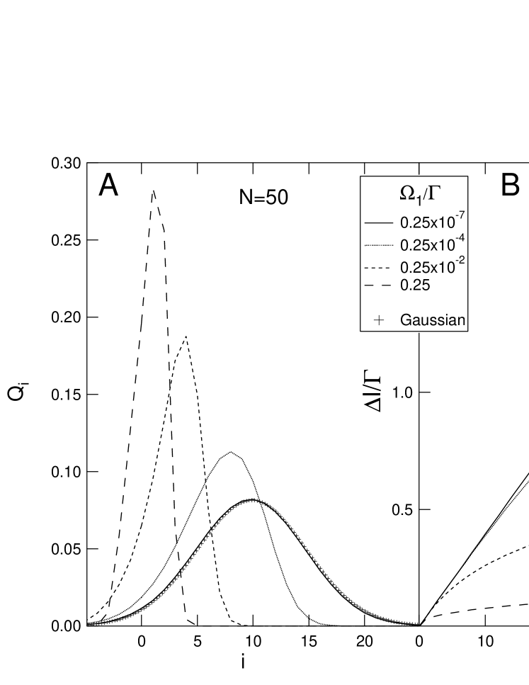
Figure 6: A: Probability distribution functions of the nanoparticle many-electron states in the antiparallel state, when the number of energy levels available to tunnel in is $N=50$. B: Spin-polarized current $\Delta I=I_{\uparrow\uparrow}-I_{\uparrow\downarrow}$ versus $N$, the number of energy levels available to tunnel in. $N$ and bias voltage are related linearly. 

The distribution mode is now obtained from

$$N\frac{2P}{1+P^{2}}=i_{0}+\frac{1.6\Omega_{1}i_{0}^{5}}{\Gamma(1+P^{2})}.$$ (30)

At large N, when the spin relaxation term dominates,

$$i_{0}\approx\left(\frac{2PN\Gamma}{1.6\Omega_{1}}\right)^{1/5},$$

that is, the mode crosses over from being linear with $N$ to being proportional to $N^{1/5}$.

Fig. 6-B displays spin-polarized current versus $N$ obtained by numerical calculations, for different $\Omega_{1}/\Gamma$. The crossover from linear to a much weaker dependence is evident for $\Omega_{1}/\Gamma=0.25$ and $0.25\cdot 10^{-2}$. The crossovers in $i_{0}$ and $I_{\uparrow\uparrow}-I_{\uparrow\downarrow}$ are equivalent, as discussed before, so at large $N$, $I_{\uparrow\uparrow}-I_{\uparrow\downarrow}\sim N^{1/5}$.

At $\Omega_{1}/\Gamma=0.25$, the rate of spin-relaxation with energy difference $\delta$ is small compared to the tunneling rate. But $\Omega_{2}/\Gamma=11.5$, so the spin-relaxation rate with an energy difference $\geq 2\delta$ is large compared to the tunneling rate. As a result, the spin-polarized current crosses over already at the second single electron energy level. In particular, we find that the contribution from the second single-electron energy level to the spin polarized current is approximately a 3rd of the contribution from the first single-electron energy level.

VIII Fitting

To illustrate how the model derived in this paper can be used to interpret measurements of the spin-polarized current, we discuss sample 1 in Ref. Wei et al. (2007). In Fig. 7-A we display the I-V curve at $T=0.03K$, obtained in the parallel magnetization configuration and in the regime where the electron discharge rate is much faster than the tunnel in rate, as required by our model (we have reversed the sign of bias voltage compared to that in Ref. Wei et al. (2007)). The I-V curve increases in discrete steps at voltages corresponding to discrete energy levels of the nanoparticle. The average tunnel in rate is obtained as $\Gamma=<\delta I>/2|e|=1.5MHz$, Wei et al. (2007) where $<\delta I>$ is the average current step. The average level spacing $\delta=0.8meV$ corresponds to a spherical nanoparticle with diameter 6nm. The electron g-factors are very close to 2, Wei et al. (2007) confirming weak spin-orbit scattering.

The spin polarized current, $\Delta I=I_{\uparrow\uparrow}-I_{\uparrow\downarrow}$, versus $N$ is shown by circles in Fig. 7-B. At small $N$, energy levels are well resolved, and $N$ is observed directly as shown in the figure. At large bias voltage, where energy levels are broadened, we find $N$ as $ec(V-V_{CB})/\delta$, Wei et al. (2007) where $c$ is the capacitance ratio that converts from voltage to nanoparticle energy and $V_{CB}$ is the Coulomb blockade voltage threshold.

We fit $\Delta I$ obtained from the model versus $N$, using a fixed tunnel rate $\Gamma=1.5MHz$ and two fit parameters, $P$ and $\Omega_{1}$. We assume $\Omega_{i}\approx 1.6i^{5}\Omega_{1}$, which is valid when spin relaxation is mediated by phonons following Elliot-Yafet scaling, as discussed earlier. The best fit parameters are $P=0.23$ and $\Omega_{1}=1.1\Gamma\approx 1.6MHz$. This value of the spin-relaxation rate is consistent with what we estimated based on qualitative discussions in Ref. Wei et al. (2007)

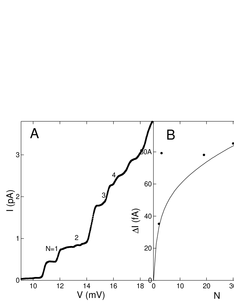
Figure 7: A: I-V curve in sample 1 near the sequential tunneling threshold. B: Circles: Spin polarized current $\Delta I=I_{\uparrow\uparrow}-I=I_{\uparrow\downarrow}$ versus $N$. Line is the best fit to the model. 

The best fit does not fully saturate with bias voltage, as seen in Fig. 6-B and  7-B, but exhibits a crossover to a weaker dependence with $N$. Nevertheless, we find the agreement between the model and the data to be qualitatively good. An outlying point at $N=3$ in Fig. 7-B is attributed to the large tunnel rate via the third energy levels as seen in Fig. 7-A, because we use a constant tunnel in rate in the fit. Such a large tunnel in rate arises from the natural statistical fluctuations of the tunnel rates among different levels.

If we assume that the spin-relaxation rate is energy independent, $\Omega_{i}=\Omega_{1}$, the spin-polarized current in our model will have a linear dependence with $N$. In that case, not only does the best fit have five times larger chi-square, but also the best fit parameters are un-physical, $P=0.045$ and $\Omega_{1}=0.067\Gamma$. In particular, the measured spin-polarized current via the low energy levels would be 25 times larger than the maximum theoretical value corresponding to $TMR=2P^{2}/(1+P^{2})$ at $P=0.045$. Consequently, an energy independent spin-relaxation rate cannot explain our results, and the energy dependence of the spin-relaxation rate plays a critical role in interpreting the spin-polarized current through the nanoparticle in the regime of well resolved energy levels and weak spin-orbit scattering.

Our model neglects higher order spin relaxation processes. We suggest that there could also be transitions where two electrons flip their spin simultaneously, emitting a phonon with angular momentum $2\hbar$. The probability of such a transition path must be much weaker relative to the probability of the 1st order process (weaker by a factor of $\alpha$) . But with increasing $i$, the number of transition paths behind a second-order process would increase much faster with $i$ than in $\Omega_{i}$, leading to a larger exponent in the dependence of the spin-relaxation rate on $i$. As a result, at high excitation energies, second order or even higher order spin-relaxation process can dominate spin-relaxation, leading to another crossover in $\Delta I$ versus $V$, weakening the $V$ dependence further. Thus, inclusion of the the higher order spin-relaxation processes at high excitation energies would improve the agreement between model and measurements.

IX Conclusion

In conclusion, we have derived a simple model for calculating spin-accumulation and spin-polarized current via discrete energy levels of a metallic nanoparticle in the regime of weak spin-orbit scattering. The model is valid in a relatively narrow range of sample parameters. However, a large percentage of samples fabricated by lithography have parameters in that range. The energy dependence of the spin-relaxation rate causes a significant suppression of the bias voltage dependence of the spin-polarized current at large bias voltage. In particular, if the spin-relaxation rate increases with excitation energy as a power of $n$, $\nu^{SF}(\omega)\sim\omega^{n}$, then the spin polarized current at large bias voltage $V$ will increase proportionally to $V^{1/(n+2)}$, which is a dependence much weaker than linear. The crossover between the linear dependence at low voltage and the much weaker dependence at large voltage occurs when the the spin-polarized current$/|e|$ is equal to the spin-relaxation rate with the energy difference given by the spin-accumulation. The model leads to the spin-relaxation rate $1.6MHz$ in an Aluminum nanoparticle of diameter $6nm$, for a transition with an energy difference of one level spacing.

This work was performed in part at the Georgia-Tech electron microscopy facility. This research is supported by the DOE grant DE-FG02-06ER46281 and David and Lucile Packard Foundation grant 2000-13874.

X Appendix: Masters Equation

In the steady state the occupational probabilities are time-independent and the masters equation 5 becomes

$$Q_{\alpha}\sum_{{\beta\neq\alpha}}\Gamma_{{\alpha}\to{\beta}}=\sum_{{\beta}\neq\alpha}Q_{\beta}\Gamma_{{\beta}\to{\alpha}}.$$ (31)

The occupational probabilities satisfy the normalization condition $\sum_{\alpha}Q_{\alpha}=1$.

In this section we reduce the problem of solving Eq. 31 into a simpler problem. This is done by identifying a group of states which have much larger probability than the states outside the group and then eliminating the occupational probabilities of the states outside the group.

We use inequalities $\nu_{\alpha\to\beta}\gg\Gamma^{R}\gg\max(\Gamma^{L},\nu_{\alpha\to\beta}^{SF})$. $\nu_{\alpha\to\beta}$ is the spin-conserving relaxation rate from state $|\alpha>$ to state $|\beta>$ given by Eq 4, in which $\omega=E_{\alpha}-E_{\beta}$ is the energy difference between the initial and the final state. We calculate at zero temperature, so $\nu_{\alpha\to\beta}=0$ if $E_{\alpha}<E_{\beta}$. $\nu_{\alpha\to\beta}$ is nonzero only if the initial and the final state have the same spin. In this regime the electron transport through the nanoparticle is in equilibrium with respect to spin-conserving relaxation.

$\nu_{\alpha\to\beta}^{SF}$ is the spin-flip relaxation rate between the states. It can be calculated using Eq. 2. $\nu_{\alpha\to\beta}^{SF}$ is nonzero only if $S_{\beta}^{z}-S_{\alpha}^{z}=\pm\hbar$.

In the analysis, we separate the states that are fully relaxed with respect to spin-conserving relaxation processes from those that are not. The latter states decay at rate $\nu_{\alpha\to\beta}$, whereas the former states decay at a rate $\max{(\Gamma^{L},\nu^{SF})}$ or $\Gamma^{R}$, depending on weather the number of electrons is even (before tunneling in after tunneling out) or odd (after tunneling in before tunneling out). From Eq. 31 it follows that the occupational probabilities of states that are not fully relaxed with respect to spin-conserving transitions are strongly suppressed in the limit $\nu_{\alpha\to\beta}\gg\Gamma^{R}\gg\max(\Gamma^{L},\nu_{\alpha\to\beta}^{SF})$, because the occupational probability of those states have $\nu_{\alpha\to\beta}$ in the denominator.

We are considering only the states with one extra added electron, as discussed in sections  IV and  V. Let $Q_{i}$ denote the occupational probabilities of the states without an added extra electron that are fully relaxed by spin-conserving transitions. These states are from group $G_{1}$ and are shown in Fig. 3. Let $P_{j}$ denote the occupational probabilities of the states with an added extra electron that are fully relaxed by spin-conserving transitions; these states are from group $G_{3}$.

Next we consider the excited states. $Q^{\prime}_{\alpha}$ denotes the occupational probabilities of the states without an added electron that are not fully relaxed by spin-conserving transitions; these are the states from group $G_{2}$. Finally, $P^{\prime}_{\beta}$ denotes the occupational probabilities of the states with an added extra electron that are not fully relaxed by spin-conserving transitions; these are states from group $G_{4}$.

The masters equations are next written for the states in each group. For groups 1 and 2, the equations are

$$Q_{i}\bigg{[}\sum_{m\in G_{1}}\nu_{i\to m}^{SF}+\sum_{\alpha^{\prime}\in G_{2}}\nu_{i\to\alpha^{\prime}}^{SF}$$

$$+\sum_{j^{\prime}\in G_{3}}\Gamma_{i\to j^{\prime}}+\sum_{\beta^{\prime}\in G_{4}}\Gamma_{i\to\beta^{\prime}}\bigg{]}$$

$$=\sum_{m\in G_{1}}Q_{m}\nu_{m\to i}^{SF}+\sum_{\alpha^{\prime}\in G_{2}}Q^{\prime}_{\alpha^{\prime}}(\nu_{\alpha^{\prime}\to i}+\nu_{\alpha^{\prime}\to i}^{SF})$$

$$+\sum_{j^{\prime}\in G_{3}}P_{j^{\prime}}\Gamma_{j^{\prime}\to i}+\sum_{\beta^{\prime}\in G_{4}}P^{\prime}_{\beta^{\prime}}\Gamma_{\beta^{\prime}\to i},$$ (32)

$$Q^{\prime}_{\alpha}\bigg{[}\sum_{m\in G_{1}}(\nu_{\alpha\to m}+\nu_{\alpha\to m}^{SF})+\sum_{\alpha^{\prime}\in G_{2}}(\nu_{\alpha\to\alpha^{\prime}}+\nu_{\alpha\to\alpha^{\prime}}^{SF})$$

$$+\sum_{j^{\prime}\in G_{3}}\Gamma_{\alpha\to j^{\prime}}+\sum_{\beta^{\prime}\in G_{4}}\Gamma_{\alpha\to\beta^{\prime}}\bigg{]}$$

$$=\sum_{m\in G_{1}}Q_{m}\nu_{m\to\alpha}^{SF}+\sum_{\alpha^{\prime}\in G_{2}}Q^{\prime}_{\alpha^{\prime}}(\nu_{\alpha^{\prime}\to\alpha}+\nu_{\alpha^{\prime}\to\alpha}^{SF})$$

$$+\sum_{j^{\prime}\in G_{3}}P_{j^{\prime}}\Gamma_{j^{\prime}\to\alpha}+\sum_{\beta^{\prime}\in G_{4}}P^{\prime}_{\beta^{\prime}}\Gamma_{\beta^{\prime}\to\alpha},$$ (33)

where $i\in G_{1}$, $\alpha\in G_{2}$. Rates $\Gamma_{i\to j^{\prime}}$, $\Gamma_{i\to\beta^{\prime}}$, $\Gamma_{\alpha\to j^{\prime}}$, and $\Gamma_{\alpha\to\beta^{\prime}}$ on the left hand sides are proportional to the tunnel-in rate $\Gamma^{L}$ across the left junction. Similarly, rates $\Gamma_{j^{\prime}\to i}$, $\Gamma_{\beta^{\prime}\to i}$, $\Gamma_{\alpha\to j^{\prime}}$, and $\Gamma_{\beta^{\prime}\to\alpha}$ on the right hand sides are proportional to the tunnel-out rate $\Gamma^{R}$ across the left junction.

For groups 3 and 4, the equations are

$$P_{j}\bigg{[}\sum_{m\in G_{1}}\Gamma_{j\to m}+\sum_{\alpha^{\prime}\in G_{2}}\Gamma_{j\to\alpha^{\prime}}$$

$$+\sum_{j^{\prime}\in G_{3}}\nu_{j\to j^{\prime}}^{SF}+\sum_{\beta^{\prime}\in G_{4}}\nu_{j\to\beta^{\prime}}^{SF}\bigg{]}$$

$$=\sum_{m\in G_{1}}Q_{m}\Gamma_{m\to j}+\sum_{\alpha^{\prime}\in G_{2}}Q^{\prime}_{\alpha^{\prime}}\Gamma_{\alpha^{\prime}\to j}+$$

$$\sum_{j^{\prime}\in G_{3}}P_{j^{\prime}}\nu_{\j^{\prime}\to j}^{SF}+\sum_{\beta^{\prime}\in G_{4}}P^{\prime}_{\beta^{\prime}}(\nu_{\beta^{\prime}\to j}+\nu_{\beta^{\prime}\to j}^{SF}),$$ (34)

$$P^{\prime}_{\beta}\bigg{[}\sum_{m\in G_{1}}\Gamma_{\beta\to m}+\sum_{\alpha^{\prime}\in G_{2}}\Gamma_{\beta\to\alpha^{\prime}}$$

$$+\sum_{j^{\prime}\in G_{3}}(\nu_{\beta\to j^{\prime}}+\nu_{\beta\to j^{\prime}}^{SF})+\sum_{\beta^{\prime}\in G_{4}}(\nu_{\beta\to\beta^{\prime}}+\nu_{\beta\to\beta^{\prime}}^{SF})\bigg{]}$$

$$=\sum_{m\in G_{1}}Q_{m}\Gamma_{m\to\beta}+\sum_{\alpha^{\prime}\in G_{2}}Q^{\prime}_{\alpha^{\prime}}\Gamma_{\alpha^{\prime}\to\beta}+$$

$$\sum_{j^{\prime}\in G_{3}}P_{j^{\prime}}\nu_{\j^{\prime}\to\beta}^{SF}+\sum_{\beta^{\prime}\in G_{4}}P^{\prime}_{\beta^{\prime}}(\nu_{\beta^{\prime}\to\beta}+\nu_{\beta^{\prime}\to\beta}^{SF}),$$ (35)

where $j\in G_{3}$, $\beta\in G_{4}$.

First we estimate the orders of magnitude of the occupational probabilities. The transition rates are assumed roughly constant to within an order of magnitude and pulled out of the sum, and $Q$, $Q^{\prime}$, $P$, and $P^{\prime}$ refer to the probability of finding the particle in a state from group 1, 2, 3, and 4, respectively.  Entering the orders of magnitude of various terms in Eq. 33, we obtain $Q^{\prime}(\nu+\nu^{SF}+\Gamma^{L})\sim Q\nu^{SF}+Q^{\prime}(\nu+\nu^{SF})+P\Gamma^{R}+P^{\prime}\Gamma^{R}$, where $\nu$ and $\nu^{SF}$ indicate orders of magnitude of $\nu_{\alpha\to\beta}$ and $\nu_{\alpha\to\beta}^{SF}$, respectively. In the limit $\nu\gg\Gamma^{R}\gg\max(\Gamma^{L},\nu^{SF})$, one gets $Q^{\prime}\nu\sim Q\nu^{SF}+(P+P^{\prime})\Gamma^{R}$.

Similarly, substituting orders of magnitude in Eq. 32, one obtains $Q(\nu^{SF}+\Gamma^{L})\sim Q\nu^{SF}+Q^{\prime}(\nu+\nu^{SF})+P\Gamma^{R}+P^{\prime}\Gamma^{R}$. In the limit $\nu\gg\Gamma^{R}\gg\max(\Gamma^{L},\nu^{SF})$, one gets $Q(\nu^{SF}+\Gamma^{L})\sim Q^{\prime}\nu+(P+P^{\prime})\Gamma^{R}$. Combining the two order of magnitude estimates we obtain

$$Q^{\prime}\sim Q\frac{\nu^{SF}+\Gamma^{L}}{\nu}\approx Q\frac{\max(\nu^{SF},\Gamma^{L})}{\nu}\ll Q.$$ (36)

Hence, the occupational probabilities $Q_{\alpha}^{\prime}$ of the excited states from group $G_{2}$ are much smaller than the occupational probabilities $Q_{i}$ of states that are fully relaxed with respect to spin-conserving transitions, an expected result.

Next, we substitute into Eq. 35 the orders of magnitude of various terms and obtain $P^{\prime}(\Gamma^{R}+\nu+\nu^{SF})\sim Q\Gamma^{L}+Q^{\prime}\Gamma^{L}+P\nu^{SF}+P^{\prime}(\nu+\nu^{SF})$. Using $\nu\gg\Gamma^{R}\gg\max(\Gamma^{L},\nu^{SF})$ and Eq. 36, one obtains $P^{\prime}\nu\sim Q\Gamma^{L}+P\nu^{SF}$. Finally, Eq. 34 leads to order of magnitude estimate $P(\Gamma^{R}+\nu+\nu^{SF})\sim Q\Gamma^{L}+Q^{\prime}\Gamma^{L}+P\nu^{SF}+P^{\prime}(\nu+\nu^{SF})$, which leads to $P\Gamma^{R}\sim Q\Gamma^{L}+P^{\prime}\nu$. Combining the estimates, we obtain

$$P\sim Q\frac{\Gamma^{L}}{\Gamma^{R}}\ll Q,P^{\prime}\sim P\frac{\Gamma^{R}}{\nu}\ll P.$$ (37)

So, the occupational probabilities of states with an added electron and fully relaxed with respect to spin-conserving transitions are much smaller than the occupational probabilities of states without an added electron and fully relaxed with respect to spin-conserving transitions, as expected from the large asymmetry in tunnel resistance. In addition, the occupational probabilities of excited states with an added electron are much smaller than the occupational probabilities of states with an added electron and fully relaxed with respect to spin-conserving transitions.

Using the estimates in Eq. 36 and  37, the leading order of the masters equation for groups 1 and 2 are

$$Q_{i}\bigg{[}\sum_{m\in G_{1}}\nu_{i\to m}^{SF}+\sum_{\alpha^{\prime}\in G_{2}}\nu_{i\to\alpha^{\prime}}^{SF}$$

$$+\sum_{j^{\prime}\in G_{3}}\Gamma_{i\to j^{\prime}}+\sum_{\beta^{\prime}\in G_{4}}\Gamma_{i\to\beta^{\prime}}\bigg{]}$$

$$=\sum_{m\in G_{1}}Q_{m}\nu_{m\to i}^{SF}+\sum_{\alpha^{\prime}\in G_{2}}Q^{\prime}_{\alpha^{\prime}}\nu_{\alpha^{\prime}\to i}$$

$$+\sum_{j^{\prime}\in G_{3}}P_{j^{\prime}}\Gamma_{j^{\prime}\to i},$$ (38)

$$Q^{\prime}_{\alpha}\bigg{[}\sum_{m\in G_{1}}\nu_{\alpha\to m}+\sum_{\alpha^{\prime}\in G_{2}}\nu_{\alpha\to\alpha^{\prime}}\bigg{]}$$

$$=\sum_{m\in G_{1}}Q_{m}\nu_{m\to\alpha}^{SF}+\sum_{\alpha^{\prime}\in G_{2}}Q^{\prime}_{\alpha^{\prime}}\nu_{\alpha^{\prime}\to\alpha}$$

$$+\sum_{j^{\prime}\in G_{3}}P_{j^{\prime}}\Gamma_{j^{\prime}\to\alpha},$$ (39)

where $i\in G_{1}$, $\alpha\in G_{2}$. For groups 3 and 4, the equations are

$$P_{j}\bigg{[}\sum_{m\in G_{1}}\Gamma_{j\to m}+\sum_{\alpha^{\prime}\in G_{2}}\Gamma_{j\to\alpha^{\prime}}\bigg{]}$$

$$=\sum_{m\in G_{1}}Q_{m}\Gamma_{m\to j}+\sum_{\beta^{\prime}\in G_{4}}P^{\prime}_{\beta^{\prime}}\nu_{\beta^{\prime}\to j},$$ (40)

$$P^{\prime}_{\beta}\bigg{[}\sum_{j^{\prime}\in G_{3}}\nu_{\beta\to j^{\prime}}+\sum_{\beta^{\prime}\in G_{4}}\nu_{\beta\to\beta^{\prime}}\bigg{]}$$

$$=\sum_{m\in G_{1}}Q_{m}\Gamma_{m\to\beta}+\sum_{\beta^{\prime}\in G_{4}}P^{\prime}_{\beta^{\prime}}\nu_{\beta^{\prime}\to\beta},$$ (41)

where $j\in G_{3}$, $\beta\in G_{4}$. The relative errors of the terms in these equations are smaller than the maximum of $\max(\Gamma^{L},\nu^{SF})/\nu$, $\Gamma_{L}/\Gamma_{R}$, $\nu^{SF}/\Gamma_{R}$, and $\Gamma_{R}/\nu$.

Now we begin the process of elimination. The first step is to eliminate the excited states. In principle, the space of excited states is very large, if the excited states include multiple electron hole pairs. Agam et al. (1997) These multiply excited states are generated by tunneling if the particle remains excited longer than the time of a sequential tunneling cycle, so in our limit the occupational probabilities of the excited states with multiple electron-hole pairs are negligibly small. In this regime, the space of excited states $G_{2}$ can be restricted to the excited states that can undergo a direct spin-conserving transition into a state from $G_{1}$. Similarly, the space of excited states $G_{4}$ can be restricted to those excited states that can undergo a direct spin-conserving transition into a state from $G_{3}$.

Consider Eq. 41, which represents an equilibrium condition for a state $|\beta>$, $\beta\in G_{4}$. For a given state $|j>$, $j\in G_{3}$, we select a subspace within $G_{4}$, such that the nanoparticle in a state from the subspace can relax via spin-conserving transition into the state $|j>$. That is, for any state $|\beta>$ within the subspace, $\nu_{\beta\to j}\neq 0$, and for any state $|\beta>$ outside the subspace, $\nu_{\beta\to j}=0$. Then we sum Eq. 41 over the subspace, which leads to

$$\sum_{\beta\in G_{4}}^{\prime}\sum_{j^{\prime}\in G_{3}}P^{\prime}_{\beta}\nu_{\beta\to j^{\prime}}+\sum_{\beta\in G_{4}}^{\prime}\sum_{\beta^{\prime}\in G_{4}}P^{\prime}_{\beta}\nu_{\beta\to\beta^{\prime}}=$$

$$\sum_{m\in G_{1}}\sum_{\beta\in G_{4}}^{\prime}Q_{m}\Gamma_{m\to\beta}+\sum_{\beta\in G_{4}}^{\prime}\sum_{\beta^{\prime}\in G_{4}}P^{\prime}_{\beta^{\prime}}\nu_{\beta^{\prime}\to\beta},$$

where $\sum_{\beta\in G_{4}}^{\prime}$ sums only over the states within the subspace, so that $\nu_{\beta\to j}\neq 0$.

In the second term on the left hand side of this equation, where $\beta$ is restricted within the subspace, $\beta^{\prime}$ becomes also restricted within the subspace, because of the spin-conservation (since states $|\beta>$ and $|j>$ have the same spin, and states $|\beta^{\prime}>$ and $|\beta>$ also have the same spin, $\beta^{\prime}$ must be restricted within the subspace). The second term becomes $\sum_{\beta,\beta^{\prime}\in G_{4}}^{\prime}P^{\prime}_{\beta}\nu_{\beta\to\beta^{\prime}}$. Similarly, in the second term on the right hand side, $\nu_{\beta^{\prime}\to\beta}$ is nonzero only if states $|\beta^{\prime}>$ and $|\beta>$ have the same spin as the spin in state $|j>$, and the term becomes $\sum_{\beta,\beta^{\prime}\in G_{4}}^{\prime}P^{\prime}_{\beta^{\prime}}\nu_{\beta^{\prime}\to\beta}$. Exchanging the indices $\beta$ and $\beta^{\prime}$, the second terms on the left hand side and the right hand side cancel.

Now consider the first term on the left hand side. As stated above, only those states $|\beta>$ that can undergo a spin-conserving transition into the state $|j>$ are in the sum over $\beta$. It follows that $\nu_{\beta\to j^{\prime}}$ is nonzero only if $j^{\prime}=j$, since varying states $|j^{\prime}>$ from space $G_{3}$ have different spin. The first term on the left hand side becomes $\sum_{\beta\in G_{4}}^{\prime}P^{\prime}_{\beta}\nu_{\beta\to j}$. We can remove the prime and sum instead over the entire space $G_{4}$, because $\nu_{\beta\to j}$ automatically restricts the sum to the subspace. One obtains

$\sum_{\beta\in G_{4}}P^{\prime}_{\beta}\nu_{\beta\to j}=\sum_{m\in G_{1}}Q_{m}\sum_{\beta\in G_{4}}^{\prime}\Gamma_{m\to\beta}.$

The left hand side in this equation is the same as the second term on the right hand side of Eq. 40 and thus it can be eliminated, which leads to

$$P_{j}=\sum_{m\in G_{1}}Q_{m}\frac{\Gamma_{m\to j}+\sum_{\beta\in G_{4}}^{\prime}\Gamma_{m\to\beta}}{\sum_{m\in G_{1}}\Gamma_{j\to m}+\sum_{\alpha^{\prime}\in G_{2}}\Gamma_{j\to\alpha^{\prime}}}.$$ (42)

Next we perform a similar elimination process using Eqs. 38 and  39. For a given $i\in G_{1}$, we sum Eq. 39 over the excited states $|\alpha>$, $\alpha\in G_{2}$, for which $\nu_{\alpha\to i}\neq 0$,

$$\sum_{\alpha\in G_{2}}^{\prime}\sum_{m\in G_{1}}Q^{\prime}_{\alpha}\nu_{\alpha\to m}+\sum_{\alpha\in G_{2}}^{\prime}\sum_{\alpha^{\prime}\in G_{2}}Q^{\prime}_{\alpha}\nu_{\alpha\to\alpha^{\prime}}=$$

$$\sum_{\alpha\in G_{2}}^{\prime}\sum_{m\in G_{1}}Q_{m}\nu_{m\to\alpha}^{SF}+\sum_{j\in G_{3}}\sum_{\alpha\in G_{2}}^{\prime}P_{j}\Gamma_{j\to\alpha}+$$

$$\sum_{\alpha\in G_{2}}^{\prime}\sum_{\alpha^{\prime}\in G_{2}}Q^{\prime}_{\alpha^{\prime}}\nu_{\alpha^{\prime}\to\alpha}.$$

Following a similar analysis to that above, the second term on the left hand side is equal to the third term on the right hand side, and the first term is nonzero only for $m=i$, so one obtains

$\sum_{\alpha\in G_{2}}Q^{\prime}_{\alpha}\nu_{\alpha\to i}=\sum_{m\in G_{1}}Q_{m}\sum_{\alpha\in G_{2}}^{\prime}\nu_{m\to\alpha}^{SF}+\sum_{j\in G_{3}}P_{j}\sum_{\alpha\in G_{2}}^{\prime}\Gamma_{j\to\alpha}.$

Substituting this equation and Eq. 42 into Eq. 38, and following several lines of algebra, one obtains the renormalized masters equation in the space of states $G_{1}$, with the renormalized rate

$$\Gamma_{m\to i}^{ren}=\nu_{m\to i}^{SF}+\sum_{\alpha\in G_{2}}^{\nu_{\alpha\to i}\neq 0}\nu_{m\to\alpha}^{SF}$$

$$+\sum_{j\in G_{3}}(\Gamma_{m\to j}+\sum_{\beta\in G_{4}}^{\nu_{\beta\to j}\neq 0}\Gamma_{m\to\beta})$$

$$\times\frac{\Gamma_{j\to i}+\sum_{\alpha\in G_{2}}^{\nu_{\alpha\to i}\neq 0}\Gamma_{j\to\alpha}}{\sum_{m^{\prime}\in G_{1}}\Gamma_{j\to m^{\prime}}+\sum_{\alpha\in G_{2}}\Gamma_{j\to\alpha}}$$ (43)

This expression is the same as that obtained intuitively in the main text. The right hand side in the first row is the renormalized spin-flip rate, $\Omega_{m\to i}=\nu_{m\to i}^{SF}+\sum_{\alpha\in G_{2}}^{\nu_{\alpha\to i}\neq 0}\nu_{m\to\alpha}^{SF}$. $\nu_{m\to i}^{SF}$ is the direct spin-flip transition rate and the sum is taken over the excited states that can undergo a spin-conserving transition into the final state $|i>$.

In the spin-flip process the spin decreases by $\hbar$, hence $\nu_{m\to\i}^{SF}\neq 0$ only if $\Delta S_{z}=S_{z}^{i}-S_{z}^{m}=-\hbar$, and $\nu_{m\to\alpha}^{SF}\neq 0$ only if $\Delta S_{z}=S_{z}^{\alpha}-S_{z}^{m}=-\hbar$. It follows that $\Omega_{m\to i}\neq 0$ only if $i=m-1$. In that case, one can denote $\Omega_{m\to m-1}=\Omega_{m}=\nu_{m\to m-1}^{SF}+\sum_{\alpha\in G_{2}}^{\nu_{\alpha\to m-1}\neq 0}\nu_{m\to\alpha}^{SF}$. $\Omega_{m}$ in this equation is the renormalized spin-flip rate given by Eq. 27.

Next we examine the second and the third row of Eq. 43. The sum over $j$ is taken over intermediate states with an extra added electron. Writing the rates $\Gamma_{x\to y}$ explicitly (which is not shown here), it can be seen that the rates of tunneling in to the various unoccupied single electron states are multiplied by the rates of tunneling-out from the various occupied single electron states. The contribution to $\Gamma_{m\to i}^{ren}$ is nonzero only if $i=m-1$ or $i=m$ or $i=m+1$, because a sequential tunneling process changes the spin by $-1$ or $0$ or $1$.

Consider the expression $\Gamma_{m\to m+1}^{ren}$ in Eq. 43. In the second row term $\sum_{j\in G_{3}}(\Gamma_{m\to j}+\sum_{\beta\in G_{4}}^{\nu_{\beta\to j}\neq 0}\Gamma_{m\to\beta})\times(...)$, $j$ indicates the state obtained by adding an electron into the lowest unoccupied single-electron level with spin up. The sum over $\beta$ is taken over the excited states that can relax via spin-conserving transition into $|j>$. One obtains $\sum_{j\in G_{3}}(\Gamma_{m\to j}+\sum_{\beta\in G_{4}}^{\nu_{\beta\to j}\neq 0}\Gamma_{m\to\beta})\times(...)=\sum_{k=m+1}^{N}\Gamma_{k}(1+P)\times(...)$, where $\Gamma_{k}$ is the tunnel-in rate across the left lead into an unoccupied single-electron energy level $k$. This expression is the same as that in Eq. 9.

The third row in Eq. 43 can be interpreted as the probability that the nanoparticle in state $j$ will discharge a spin-down electron, which is the same as $\pi_{i}(\downarrow)$ in Eq. 9. Substituting the tunnel rates into Eq. 43 explicitly, one obtains that the third row of Eq. 43 is the same as Eq. 10.

In summary, the model of electron transport from the intuitive approach is derived in this appendix, using the masters equations.

References

- Seneor et al. (2007) P. Seneor, A. Bernand-Mantel, and F. Petroff, J. Phys.: Condens. Matter 99, 165222 (2007).
- Ernult et al. (2007) F. Ernult, K. Yakushiji, S. Mitani, and K. Takanashi, J. Phys. Cond. Mat. 19, 1652140 (2007).
- Johnson and Silsbee (1985) M. Johnson and R. H. Silsbee, Phys. Rev. Lett. 55, 1790 (1985).
- Jedema et al. (2001) F. J. Jedema, A. T. Filip, and B. J. van Wees, Nature 410, 345 (2001).
- Bernand-Mantel et al. (2006) A. Bernand-Mantel, P. Seneor, N. Lidgi, M. Munoz, V. Cros, S. Fusil, K. Bouzehouane, C. Deranlot, A. Vaures, F. Petroff, et al., Appl. Phys. Lett. 89, 062502 (2006).
- Wei et al. (2007) Y. G. Wei, C. E. Malec, and D. Davidovic, Phys. Rev. B 76, 195327 (2007).
- Barnas and Fert (1998a) J. Barnas and A. Fert, Phys. Rev. Lett. 80, 1058 (1998a).
- Majumdar and Hershfield (1998) K. Majumdar and S. Hershfield, Phys. Rev. B 57, 11521 (1998).
- Barnas and Fert (1998b) J. Barnas and A. Fert, Europhysics letters 44, 85 (1998b).
- Brataas et al. (1999a) A. Brataas, Y. V. Nazarov, J. Inoue, and G. E. W. Bauer, European physical journal B 9, 421 (1999a).
- Brataas et al. (1999b) A. Brataas, Y. V. Nazarov, J. Inoue, and G. E. W. Bauer, Phys. Rev. B 59, 93 (1999b).
- Korotkov and Safarov (1999) A. N. Korotkov and V. I. Safarov, Phys. Rev. B 59, 89 (1999).
- Barnas and Fert (1999) J. Barnas and A. Fert, J. Magn. Magn. Matter. 192, 391 (1999).
- Barnas et al. (2000) J. Barnas, J. Martinek, G. Michalek, B. R. Bulka, and A. Fert, Phys. Rev. B 62, 12363 (2000).
- Imamura et al. (1999) H. Imamura, S. Takahashi, and S. Maekawa, Phys. Rev. B 59, 6017 (1999).
- Kuo and Chen (2002) W. Kuo and C. D. Chen, Phys. Rev. B 65, 104427 (2002).
- Weymann and Barnas (2003) I. Weymann and J. Barnas, Phys. Status Solidi b 236, 651 (2003).
- Brataas and Wang (2001) A. Brataas and X. H. Wang, Phys. Rev. B 64, 104434 (2001).
- Wetzels et al. (2006) W. Wetzels, G. E. W. Bauer, and M. Grifoni, Phys. Rev. B 74, 224406 (2006).
- Weymann et al. (20053) I. Weymann, J. Konig, J. Martinek, J. Barnas, and G. Schon, Phys. Rev. B 72, 115334 (20053).
- Braun et al. (2005) M. Braun, J. Konig, and J. Martinek, Europhys. Lett. 72, 294 (2005).
- Urban et al. (2007) D. Urban, M. Braun, and J. Konig, Phys. Rev. B 76, 125306 (2007).
- van der Molen et al. (2006) S. J. van der Molen, N. Tombros, and B. J. van Wees, Phys. Rev. B 73, 220406(R) (2006).
- Matveev et al. (2000) K. A. Matveev, L. I. Glazman, and A. I. Larkin, Phys. Rev. Lett. 85, 2789 (2000).
- Brouwer et al. (2000) P. W. Brouwer, X. Waintal, and B. I. Halperin, Phys. Rev. Lett. 85, 369 (2000).
- Bonet et al. (2002) E. Bonet, M. M. Deshmukh, and D. C. Ralph, Phys. Rev. B 65, 045317 (2002).
- Yakushiji et al. (2001) K. Yakushiji, S. Mitani, K. Takanashi, S. Takahashi, S. Maekawa, H. Imamura, and H. Fujimori, Appl. Phys. Lett. 78, 515 (2001).
- Zhang et al. (2005) L. Zhang, C. Wang, Y. Wei, X. Liu, and D. Davidović, Phys. Rev. B 72, 155445 (2005).
- Yafet (1963) Y. Yafet, Sol. State Phys. 14, 1 (1963).
- Adam et al. (2002) S. Adam, M. L. Polianski, X. Waintal, and P. W. Brouwer, Phys. Rev. B 66, 195412 (2002).
- Elliot (1954) R. J. Elliot, Phys. Rev. 96, 266 (1954).
- Fabian and Sarma (1998) J. Fabian and S. D. Sarma, Phys. Rev. Lett. 81, 5624 (1998).
- Fabian and Sarma (1999) J. Fabian and S. D. Sarma, Phys. Rev. Lett. 83, 1211 (1999).
- Jedema et al. (2002) F. J. Jedema, H. B. Heersche, A. T. Filip, J. J. A. Baselmans, and B. J. van Wees, Nature 416, 713 (2002).
- Jedema et al. (2003) F. J. Jedema, M. S. Nijboer, A. T. Filip, and B. J. van Wees, Phys. Rev. B 67, 085319 (2003).
- Petta and Ralph (2001) J. R. Petta and D. C. Ralph, Phys. Rev. Lett. 87, 266801 (2001).
- Agam et al. (1997) O. Agam, N. S. Wingreen, B. L. Altshuler, D. C. Ralph, and M. Tinkham, Phys. Rev. Lett. 78, 1956 (1997).
- Ralph et al. (1995) D. C. Ralph, C. T. Black, and M. Tinkham, Phys. Rev. Lett. 74, 3241 (1995).
- Khaetskii and Nazarov (2000) A. V. Khaetskii and Y. V. Nazarov, Phys. Rev. B 61, 12639 (2000).
- Khaetskii and Nazarov (2001) A. V. Khaetskii and Y. V. Nazarov, Phys. Rev. B 64, 125316 (2001).
- Hanson et al. (2003) R. Hanson, B. Witkamp, L. Vandersypen, L. W. van Beveren, J. Elzerman, and L. Kouwenhoven, Phys. Rev. Lett. 91 (2003).
- Averin et al. (1999) D. V. Averin, A. N. Korotkov, and K. K. Likharev, Phys. Rev. B 44, 6199 (1999).
- Beenakker (1991) C. W. J. Beenakker, Phys. Rev. B 44, 1646 (1991).
- Julliere (1975) M. Julliere, Phys. Lett. A 54, 225 (1975).