Kinetic Theory for Electron Dynamics Near a Positive Ion

Abstract

A theoretical description of time correlation functions for electron properties in the presence of a positive ion of charge number $Z$ is given. The simplest case of an electron gas distorted by a single ion is considered. A semi-classical representation with a regularized electron - ion potential is used to obtain a linear kinetic theory that is asymptotically exact at short times. This Markovian approximation includes all initial (equilibrium) electron - electron and electron - ion correlations through renormalized pair potentials. The kinetic theory is solved in terms of single particle trajectories of the electron - ion potential and a dielectric function for the inhomogeneous electron gas. The results are illustrated by a calculation of the autocorrelation function for the electron field at the ion. The dependence on charge number $Z$ is shown to be dominated by the bound states of the effective electron - ion potential. On this basis, a very simple practical representation of the trajectories is proposed and shown to be accurate over a wide range including strong electron - ion coupling. This simple representation is then used for a brief analysis of the dielectric function for the inhomogeneous electron gas.

I Introduction

Electron dynamics in a rigid uniform neutralizing background is a well-studied problem (jellium in quantum mechanics fetter , one component plasma in classical mechanics hansen ). More realistically, point ions lead to a polarization of the electron density (e.g., in a hydrogen plasma) and the dynamics of the non-uniformly distributed electrons is radically changed. The objective here is to provide a practical theory for the description of equilibrium time correlation functions for electrons in the simplest case of a single point ion of charge number $Z$. If the charge is positive, essential quantum diffraction effects must be accounted for even at high temperatures and low densities to avoid the electron - ion Coulomb singularity. A classical Hamiltonian description is used here, with a regularized electron - ion interaction that accounts for such effects filinov . This study is an outgrowth of recent investigations based on molecular dynamics simulations for this system ilya . The qualitative features observed for the electron field autocorrelation function from simulation were captured by a simple mean field kinetic theory. Such a kinetic theory is obtained here from the asymptotically exact short time limit for the generator of the dynamics, providing both context and a generalization of the analysis in reference 4 to strong electron - electron coupling conditions.

The kinetic theory is solved exactly to express the correlation functions in terms of effective single electron trajectories about the ion and collective excitations via a dielectric function for the non-uniform electron fluid. For $Z=0$ the results reduce to the familiar random phase approximation (RPA) with local field effects (the generalized Vlasov approximation of reference 5; see also reference 6 for a related nonlinear kinetic equation for dusty plasmas). More generally it constitutes a generalization of the RPA to a non-uniform electron gas, with both ion - electron and electron - electron interactions renormalized by correlations (the Vlasov equation for an electron gas in a periodic potential is discussed in reference 7). The only required input is the time independent correlations for one or two electrons and the ion. For the calculations here the hypernetted chain approximation (HNC) integral equations are used for these static correlations. The correlation functions are further decomposed into contributions from the bound and free (positive and negative energy) states of the effective single particle dynamics in Section III.

As a special case, the electric field autocorrelation function is considered in Section IV with the objective of providing a clear interpretation for the $Z$ dependence observed in simulations. For increasing $Z$ this dependence includes 1) an increasing covariance of the field (initial value of the correlation function), 2) a decreasing correlation time, and 3) the development of a strong domain of anti-correlation at intermediate times ilya . It is shown here that all three features can be attributed to an increasing contribution from the bound states of the single particle effective dynamics representing actual metastable trapped trajectories of the $N$ particle dynamics. With this understanding of the active mechanisms, a simple analytic and accurate model for the bound and free state contributions is proposed and tested. The dynamics is restricted to circular and straight line trajectories, and the electron - ion charge correlation is represented by a nonlinear Debye distribution. Somewhat surprisingly, the model reproduces all of the above $Z$ dependencies with remarkable accuracy. This provides the basis for a practical representation of more general correlation functions, such as the dynamic structure factor, and more complex state conditions required for plasma spectroscopy in hot, dense matter Stambulchik ; wrighton .

To illustrate the practical utility of the model, collective excitations are explored briefly in Section VI using the model to evaluate the dielectric function for this nonuniform electron distribution about the ion. For weakly nonuniform conditions (small $Z$) the results are suggestive of a local density approximation whereby the modes are similar to those of a uniform electron gas, but with the density replaced by the actual local density near the ion. However, this simple approximation fails for larger $Z$ where the bound states dominate and long wavelength plasmons are replaced by local excitations at the circular orbit frequencies. Finally, some future directions are discussed in the last Section.

II Correlation Functions and Markovian Approximation

Consider a system of $N_{e}$ electrons of charge $-e$, an infinitely massive positive ion of charge $Ze$ placed at the origin, and a rigid uniform positive background for overall charge neutrality contained in a large volume $V$. The Hamiltonian is

$$H=\sum_{\alpha=1}^{N_{e}}\left(\frac{1}{2}mv_{\alpha}^{2}+V_{ei}\left(r_{\alpha}\right)+V_{eb}\left(r_{\alpha}\right)\right)+\frac{1}{2}\sum_{\alpha,\gamma}^{N_{e}}V_{ee}(r_{\alpha\gamma})$$ (1)

where $\mathbf{r}_{\alpha}$ and $\mathbf{v}_{\alpha}$ are the position and velocity of electron $\alpha$. The Coulomb interaction between electrons $\alpha$ and $\gamma$ is denoted by $V_{ee}(r_{\alpha\gamma})$ where $r_{\alpha\gamma}\equiv\left|\mathbf{r}_{\alpha}-\mathbf{r}_{\gamma}\right|$. Also, $V_{ei}\left(r_{\alpha}\right)$ is the electron-ion interaction for electron $\alpha$, and $V_{eb}\left(r_{\alpha}\right)$ is the Coulomb interaction for electron $\alpha$ with the uniform neutralizing background. In a quantum description, $V_{ei}\left(r_{\alpha}\right)$ is also a Coulomb interaction but in the classical case the short range attractive divergence must be “regularized” within a distance $\delta$ of the order of the de Broglie wavelength filinov . The simplest such form is ebeling

$$V_{ei}\left(r_{\alpha}\right)=-\frac{Ze^{2}}{r_{\alpha}}\left(1-e^{-r_{\alpha}/\delta}\right).$$ (2)

In the remainder of this presentation such a semi-classical description is assumed. Comments on the corresponding quantum analysis are given in the final Discussion section.

The typical response functions characterizing dynamical excitations in a plasma are the charge density or current autocorrelation functions, which are sums of single particle functions. More generally, the correlation functions of this type are defined by

$$C_{AB}(t)=\left\langle A(t)B\right\rangle=\int d\Gamma A(\Gamma_{t})B\left(\Gamma\right)\rho_{e}\left(\Gamma\right)$$ (3)

where $\Gamma=\left\{x_{1},..,x_{N_{e}}\right\}$ is a point in the $6N_{e}$ dimensional phase space, and $x_{\alpha}=\mathbf{r}_{\alpha}$,$\mathbf{v}_{\alpha}$ denotes a point in the phase space of particle $\alpha$. The notation $\Gamma_{t}$ denotes the evolution of the point $\Gamma$ to a time $t$ later under the dynamics generated by the Hamiltonian of (1). The role of the central fixed ion is suppressed in this notation, and it acts as an external potential for the electrons. The phase functions $A(\Gamma)$ and $B(\Gamma)$ denote some observables of interest, composed of sums of single particle functions.

$$A=\sum_{\alpha=1}^{N_{e}}a(x_{\alpha}),\hskip 18.06749ptB=\sum_{\alpha=1}^{N_{e}}b(x_{\alpha}).$$ (4)

Finally, the average is over an equilibrium ensemble (e.g., Gibbs), $\rho_{e}\left(\Gamma\right)$. Because of the special form (4), the $N$ particle average can be reduced to a corresponding average in the single electron subspace, by partial integration over $N_{e}-1$ electron degrees of freedom (see Appendix B)

$$C_{AB}(t)=\int dxn(r)\phi\left(v\right)a(x)\overline{b}(x,t).$$ (5)

Here, $n(r)$ is the equilibrium number density for electrons at a distance $r$ from the ion (the precise definition as a partial integral of $\rho_{e}\left(\Gamma\right)$ is given in Appendix A), and $\phi\left(v\right)$ is the Maxwell-Boltzmann velocity distribution. The function $\overline{b}(x,t)$ at $t=0$ is linearly related to the single particle phase function $b(x)$ in (4)

$$\overline{b}(x,0)=\overline{b}(x)=b(x)+\int dx^{\prime}n(\mathbf{r}^{\prime})\phi\left(v^{\prime}\right)h\left(\mathbf{r},\mathbf{r}^{\prime}\right)b(x^{\prime}).$$ (6)

The correlation function $h\left(\mathbf{r},\mathbf{r}^{\prime}\right)$ is related to the joint number density $n(\mathbf{r},\mathbf{r}^{\prime})$ for two electrons at $\mathbf{r}$ and $\mathbf{r}^{\prime}$ with the ion at the origin by

$$n(r)n(r^{\prime})h\left(\mathbf{r},\mathbf{r}^{\prime}\right)\equiv n(\mathbf{r},\mathbf{r}^{\prime})-n(r)n(r^{\prime}).$$ (7)

The precise definition for $n(\mathbf{r},\mathbf{r}^{\prime})$ as a partial integral of $\rho_{e}\left(\Gamma\right)$ is given in Appendix A. The time evolution of $\overline{b}(x,t)$ in the single particle phase space is governed by a linear equation of the form

$$\partial_{t}\overline{b}(x,t)+\int dx^{\prime}\mathcal{L}\left(x,x^{\prime};t\right)\overline{b}(x^{\prime},t)=0.$$ (8)

All of the results up to this point are still exact.

The difficult many-body problem is encountered in the determination of $\mathcal{L}\left(x,x^{\prime};t\right)$. Weak coupling and perturbation expansions are not appropriate for high $Z$ ions or conditions for strongly coupled electrons so instead a Markovian approximation is proposed,

$$\mathcal{L}\left(x,x^{\prime};t\right)\rightarrow\mathcal{L}\left(x,x^{\prime};t=0\right)\equiv\mathcal{L}\left(x,x^{\prime}\right).$$ (9)

This approximation assumes that the exact generator for the initial dynamics persists as the dominant form for later times as well. In this way the exact initial correlations among electrons and with the ion are included. The detailed form for $\mathcal{L}\left(x,x^{\prime}\right)$ is obtained in Appendix B with the result

$$\mathcal{L}\left(x,x^{\prime}\right)=\left(\mathbf{v}\cdot\nabla_{\mathbf{r}}-m^{-1}\nabla_{\mathbf{r}}\mathcal{V}_{ie}\left(r\right)\cdot\nabla_{\mathbf{v}}\right)\delta\left(x-x^{\prime}\right)+\mathbf{v}\cdot\nabla_{\mathbf{r}}\beta\mathcal{V}_{ee}\left(\mathbf{r},\mathbf{r}^{\prime}\right)\phi\left(v^{\prime}\right)n\left(r^{\prime}\right),$$ (10)

where $\mathcal{V}_{ie}\left(r\right)$ and $\mathcal{V}_{ee}\left(\mathbf{r},\mathbf{r}^{\prime}\right)$ are “renormalized” electron - ion and electron - electron interactions

$$\mathcal{V}_{ie}\left(r\right)\equiv-\beta^{-1}\ln n\left(r\right),\hskip 18.06749pt\mathcal{V}_{ee}\left(\mathbf{r},\mathbf{r}^{\prime}\right)=-\beta^{-1}c\left(\mathbf{r},\mathbf{r}^{\prime}\right).$$ (11)

The direct correlation function $c\left(\mathbf{r},\mathbf{r}^{\prime}\right)$ is defined in terms of $h\left(\mathbf{r},\mathbf{r}^{\prime}\right)$ by

$$c\left(\mathbf{r},\mathbf{r}^{\prime}\right)=h\left(\mathbf{r},\mathbf{r}^{\prime}\right)-\int d\mathbf{r}^{\prime\prime}h\left(\mathbf{r},\mathbf{r}^{\prime\prime}\right)n\left(r^{\prime\prime}\right)c\left(\mathbf{r}^{\prime\prime},\mathbf{r}^{\prime}\right).$$ (12)

At $Z=0$ this becomes the usual Ornstein - Zernicke equation hansen .

To interpret (10), substitute this approximation into (8) to get the Markovian linear kinetic equation for $\overline{b}(x,t)$

$$\left(\partial_{t}+\mathbf{v}\cdot\nabla_{\mathbf{r}}-m^{-1}\nabla_{\mathbf{r}}\mathcal{V}_{ie}\left(r\right)\cdot\nabla_{\mathbf{v}}\right)\overline{b}(x,t)=-\mathbf{v}\cdot\nabla_{\mathbf{r}}\beta\int dx^{\prime}\mathcal{V}_{ee}\left(\mathbf{r},\mathbf{r}^{\prime}\right)\phi\left(v^{\prime}\right)n\left(r^{\prime}\right)\overline{b}(x^{\prime},t).$$ (13)

At weak electron - electron coupling $\mathcal{V}_{ee}\left(\mathbf{r},\mathbf{r}^{\prime}\right)\rightarrow V_{ee}(\left|\mathbf{r}-\mathbf{r}^{\prime}\right|)$ and at weak electron - ion coupling $\mathcal{V}_{ie}\left(r\right)\rightarrow V_{ie}\left(r\right),$ and (13) is recognized as the linear Vlasov equation. More generally, the Markov approximation (13) upgrades this mean field result to include the effects of equilibrium correlations on all interaction potentials. Thus it is suitable for a discussion of the strong coupling conditions that occur for $Z>1$. The left side of (13) describes single electron motion about the ion in the effective potential $\mathcal{V}_{ie}$, while the right side describes dynamical screening of this motion.

In summary, the description of electron dynamical correlations and fluctuations has been reduced in the Markovian approximation to

$$C_{AB}(t)=\int dxn(r)\phi\left(v\right)a(x)e^{-\mathcal{L}t}\overline{b}(x),$$ (14)

where $\mathcal{L}$ is the operator whose kernel is (10). This operator requires as input the equilibrium electron density $n\left(r\right)$ and the equilibrium direct correlation function. The kinetic equation can be solved exactly in terms of the single particle trajectories about the ion and dielectric function for an inhomogeneous electron gas, describing the dynamical screening due to interactions among the electrons in the presence of the ion. The details are carried out in Appendix C, and the correlation functions are obtained from that solution in Appendix D. For the class of correlation functions for which $a(x)=a(\mathbf{r})$ (i.e., is independent of the velocity) the Laplace transform of (14) takes the simpler form

$$\int_{0}^{\infty}dte^{-zt}C_{AB}(t)=\int d\mathbf{r}d\mathbf{v}n\left(r\right)\phi\left(v\right)a(\mathbf{r};z)\mathcal{G}_{0}(z)\overline{b}(x),$$ (15)

The dynamics is governed by the resolvent operator

$$\mathcal{G}_{0}\left(z\right)=\left(z+\mathcal{L}_{0}\right)^{-1},\hskip 18.06749pt\mathcal{L}_{0}=\mathbf{v}\cdot\nabla_{\mathbf{r}}-m^{-1}\nabla_{\mathbf{r}}\mathcal{V}_{ie}\left(r\right)\cdot\nabla_{\mathbf{v}}.$$ (16)

The generator for the dynamics, $\mathcal{L}_{0},$ is seen to be that for a single electron interacting with the ion via the effective mean field potential $\mathcal{V}_{ie}\left(r\right)$. The function $a(\mathbf{r};z)$ is the given function $a(\mathbf{r})$, modified by dynamical screening

$$a(\mathbf{r};z)=\int d\mathbf{r}^{\prime}a(\mathbf{r}^{\prime})\epsilon^{-1}\left(\mathbf{r}^{\prime},\mathbf{r};z\right),$$ (17)

where $\epsilon\left(\mathbf{r},\mathbf{r^{\prime}};z\right)$ is the “dielectric function” for the electrons in the presence of the ion dielectric

$$\epsilon\left(\mathbf{r},\mathbf{r}^{\prime};z\right)=\delta\left(\mathbf{r}-\mathbf{r}^{\prime}\right)-\int d\mathbf{r}^{\prime\prime}\pi\left(\mathbf{r},\mathbf{r}^{\prime\prime};z\right)\mathcal{V}_{ee}(\mathbf{r}^{\prime\prime},\mathbf{r}^{\prime}),$$ (18)

and $\pi\left(\mathbf{r},\mathbf{r}^{\prime\prime};z\right)$ is

$$\pi\left(\mathbf{r},\mathbf{r}^{\prime\prime};z\right)=-\beta n(r)\int d\mathbf{v}\phi\left(v\right)\mathcal{G}_{0}(z)\mathbf{v}\cdot\mathbf{\nabla}_{\mathbf{r}}\delta\left(\mathbf{r}-\mathbf{r}^{\prime\prime}\right).$$ (19)

II.1 Dynamic structure factor

An important example is the autocorrelation function for the electron density near the ion. In the absence of the ion this is referred to as the dynamic structure factor and that terminology will be used here in the presence of the ion as well. The correlation function $C_{AB}(t)=C(\mathbf{q,q}^{\prime};t)$ is constructed from the local densities of (4) with $a(x_{\alpha})=\delta\left(\mathbf{q}-\mathbf{r}_{\alpha}\right)$ and $b(x_{\alpha})=\delta\left(\mathbf{q}^{\prime}-\mathbf{r}_{\alpha}\right)$. Then (15) becomes

$$\int_{0}^{\infty}dte^{-zt}C(\mathbf{q,q}^{\prime};t)=\int d\mathbf{r}d\mathbf{v}n\left(r\right)\phi\left(v\right)\epsilon^{-1}\left(\mathbf{q},\mathbf{r};z\right)\mathcal{G}_{0}\left(z\right)s\left(\mathbf{r},\mathbf{q}^{\prime}\right).$$ (20)

Here $s\left(\mathbf{r},\mathbf{q}^{\prime}\right)$ is the static structure factor

$$s\left(\mathbf{r},\mathbf{q}^{\prime}\right) = \delta\left(\mathbf{r}-\mathbf{q}^{\prime}\right)+n\left(q^{\prime}\right)h\left(\mathbf{r},\mathbf{q}^{\prime}\right)=\delta\left(\mathbf{r}-\mathbf{q}^{\prime}\right)+n\left(q^{\prime}\right)h\left(\mathbf{q}^{\prime},\mathbf{r}\right)$$ (21)

$$= \epsilon^{-1}\left(\mathbf{q}^{\prime},\mathbf{r};0\right),$$

representing the exact initial correlations. The last equality of (21) is proved in Appendix D.

Equation (20) is the exact short time (Markovian) form for the dynamic structure factor. For $Z=0$ it becomes the usual random phase approximation (RPA) with “local field corrections”; this means that the bare electron - electron potential has been replaced by $\mathcal{V}_{ee}$ (the corresponding direct correlation function) to account for exact initial correlations. The $Z=0$ case has been studied in detail for the hydrogen plasma, where this approximation is found to be very good up to moderate plasma coupling strengths over a wide range of space and time scales cauble . Equation (16) extends this approximation to include the presence of the ion for $Z\neq 0$, corresponding to an inhomogeneous RPA.

II.2 Electric field autocorrelation function

A second important example is the autocorrelation function $C(t)$ for the electron electric field at the ion, where

$$A=B=\sum_{\alpha=1}^{N_{e}}\mathbf{e}\left(\mathbf{r}_{\alpha}\right),\hskip 28.90755pt\mathbf{e}\left(\mathbf{r}_{\alpha}\right)=\nabla_{\mathbf{r}_{\alpha}}V_{ei}\left(r_{\alpha}\right).$$ (22)

This correlation function also is obtained from the dynamic structure factor $C(\mathbf{r,r}^{\prime};t)$ by integration

$$C(t)=\int d\mathbf{r}d\mathbf{r}^{\prime}\mathbf{e}\left(\mathbf{r}\right)C(\mathbf{r,r}^{\prime};t)\mathbf{e}\left(\mathbf{r}^{\prime}\right),$$

so

$$\int_{0}^{\infty}dte^{-zt}C(t)=\int d\mathbf{r}d\mathbf{v}n\left(r\right)\phi\left(v\right)\mathbf{e}(\mathbf{r};z)\cdot\mathcal{G}_{0}\left(z\right)\mathbf{e}_{s}(\mathbf{r}).$$ (23)

Interestingly, one of the fields is dynamically screened while the other is statically screened,

$$\mathbf{e}(\mathbf{r};z)=\int d\mathbf{r}^{\prime}\mathbf{e}(\mathbf{r}^{\prime})\epsilon^{-1}\left(\mathbf{r}^{\prime},\mathbf{r};z\right),\hskip 18.06749pt\mathbf{e}_{s}(\mathbf{r})=\int d\mathbf{r}^{\prime}\mathbf{e}(\mathbf{r}^{\prime})s\left(\mathbf{r}^{\prime},\mathbf{r}\right)=\mathbf{e}(\mathbf{r};z=0).$$ (24)

III Bound and free contributions

The trajectories of the mean field generator $\mathcal{L}_{0}$ do not represent the dynamics of any given electron, but rather their effective collective representation. Thus, the interactions among many electrons appears in the mean field theory only through their modification of the potentials. The bound states of the effective potential $\mathcal{V}_{ie}\left(r\right)$ are representations of real metastable states in the MD simulation. At weak coupling there are few such metastable states and their lifetimes are short compared to the correlation time for the field autocorrelation function. As $Z$ increases the stronger coupling gives rise to more metastable states with longer lifetimes. There is a crossover of these lifetimes to values larger than the correlation time at which point they behave essentially as bound states for the relevant time scales. To isolate the effects of such bound states it is useful to divide the phase space integral of (14) into contributions from bound and free parts of that phase space. The decomposition is defined by the negative and positive energy states for the effective potential $\mathcal{V}_{ie}\left(r\right)$. For a given position $r$ there is a maximum velocity $v_{m}(r)$ above which the total energy is positive

$$v_{m}(r)=\sqrt{-2\mathcal{V}_{ie}\left(r\right)/m}.$$ (25)

The single particle equilibrium density for the position and velocity can therefore be divided into two contributions

$$n(r)\phi\left(v\right) = \Theta\left(v_{m}(r)-v\right)n(r)\phi\left(v\right)+\Theta\left(v-v_{m}(r)\right)n(r)\phi\left(v\right)$$ (26)

$$= \left(n(r)\phi\left(v\right)\right)_{b}+\left(n(r)\phi\left(v\right)\right)_{f}.$$

For example, integration over the velocity gives the relative contribution of bound states to the density $n(r)$

$$n_{b}(r) \equiv \int d\mathbf{v}\left(n(r)\phi\left(v\right)\right)_{b}$$ (27)

$$= n(r)4\pi^{-\frac{1}{2}}v_{0}^{-3}\int_{0}^{v_{m}(r)}dvv^{2}e^{-\left(v/v_{0}\right)^{2}}$$

$$= n(r)\left(\mathrm{erf}\left(\frac{v_{m}(r)}{v_{0}}\right)-\frac{2}{\sqrt{\pi}}\frac{v_{m}(r)}{v_{0}}e^{-\left(v_{m}(r)/v_{0}\right)^{2}}\right).$$

where $v_{0}=\sqrt{2k_{B}T/m_{e}}$ is the thermal velocity of the electron and $\mathrm{erf}(x)$ is the error function. Since $v_{m}(r)$ is proportional to $\sqrt{Z}$, $n_{b}(r)$ is an increasing function of $Z$ for all $r$.

The decomposition (26) provides the identification of contributions to the correlation functions from bound and free states

$$C_{AB}(t)=C_{AB}^{b}(t)+C_{AB}^{f}(t).$$ (28)

The analysis of the following Sections shows that the interesting $Z$ dependence of electron dynamics can be understood in terms of the relative sizes of these two contributions.

IV Example: Electric Field Autocorrelation Function

The dielectric function $\epsilon\left(\mathbf{r},\mathbf{r}^{\prime};z\right)$ describes a crossover from no screening at short times (large $z$) to static screening at large times ($z\rightarrow 0$).  In the next two sections, the short time form with $\epsilon\left(\mathbf{r},\mathbf{r}^{\prime};z\right)\rightarrow\delta\left(\mathbf{r}-\mathbf{r}^{\prime}\right)$ will be considered. In that case the correlation functions in (15) become the effective single particle functions

$$C_{AB}(t)\rightarrow\int d\mathbf{r}d\mathbf{v}n\left(r\right)\phi\left(v\right)a(\mathbf{r})e^{-\mathcal{L}_{0}t}\overline{b}(x),$$ (29)

which are asymptotically exact at short times. The effects of dynamical screening at longer times are discussed briefly in Section VI.

The electric field autocorrelation function is particularly instructive since the field is sensitive to configurations closest to the ion. Also, its time integral determines the dominant contribution to the half width of spectral line widths broadened by electrons in many practical caseslewis . The short time form of (23) is

$$C(t)\rightarrow\int d\mathbf{r}d\mathbf{v}n\left(r\right)\phi\left(v\right)\mathbf{e}(\mathbf{r})\cdot e^{-\mathcal{L}_{0}t}\mathbf{e}_{s}(\mathbf{r}).$$ (30)

It is shown in Appendix A that the statically screened field of (24) simplifies further to

$$\mathbf{e}_{s}(\mathbf{r})=\frac{1}{Ze}\nabla_{\mathbf{r}}\mathcal{V}_{ie}\left(r\right).$$ (31)

Thus, the number density $n\left(r\right)$ determines all of the ingredients needed for calculation of $C(t)$. It is calculated here in the HNC approximation described in Appendix A. The electron - electron coupling strength is measured by the dimensionless ratio $\Gamma=\beta e^{2}/r_{0}$ where $r_{0}$ is the average distance between electrons, determined from the density by $4\pi n_{e}r_{0}^{3}/3=1$. The ion - electron coupling is measured by $\sigma=-\beta V_{ei}\left(0\right)=\beta Ze^{2}/\delta=Z\Gamma\left(r_{0}/\delta\right)$. The results presented here are for $\Gamma=0.1$, and $\sigma=0.25Z$ for values of $Z\leq 40$. The corresponding quantum regularization length is $\delta/r_{0}=0.4$. The electron - electron coupling is therefore weak, but the ion - electron coupling can be very strong, $\sigma\leq 10$. These conditions were chosen because previous molecular dynamics studies have been performed at these values ilya .

It is useful to anticipate the increasing role of bound states with increasing $Z$ by considering first the time independent covariance $C(0)$. This is shown in Figure 1. The sharp increase above $Z\sim 5$ is seen to be entirely due to the appearance of the bound states. Similar strong effects on dynamical structure are observed.

.

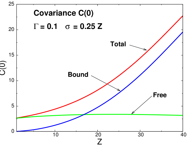
Figure 1: Bound and free state contributions to the field covariance $C(0)$ as a function of $Z$.

.

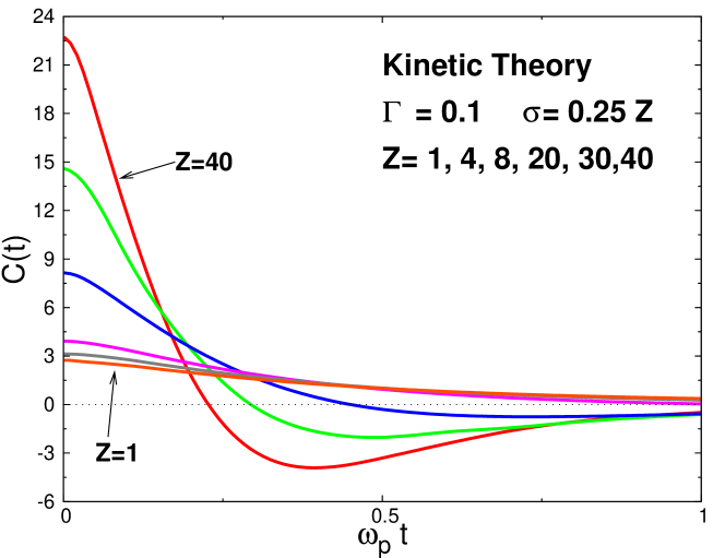
Figure 2: Autocorrelation function for an electron field at an ion of charge number $Z=1,4,8,20,30,$ and $40$

Figure 2 shows the results for $C(t)$ calculated from (30) for $Z=1,4,8,20,30,40$. The development of a strong anti-correlation and the decreasing initial correlation time with increasing $Z$ is evident. These are the effects noted above, first observed in MD simulations ilya . The interpretation of this two-fold dependence on $Z$ is provided by Figures 3 and 4 showing the contributions from bound and free state contributions for $Z=4,30$. For $Z=4$ the dominant contribution is from free states, which have a monotonic positive decay. In contrast, for $Z=30$ the dominant contribution is from bound states which provide the negative anti-correlation as the sign of the field changes along each trajectory when it passes through apsidal distances. The time for this change can be estimated by half the period for a circular orbit at position $r$, which is proportional to $\left(r^{3}/Z\right)^{1/2}$. This is consistent with the observed decrease in correlation time in Figure 2. Further elaboration and explanation is provided by the simple model of the next section.

.

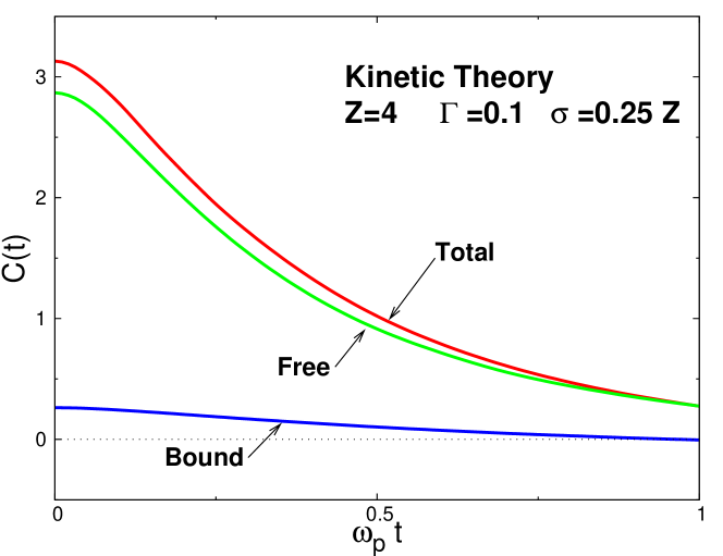
Figure 3: Bound and free state contributions to $C(t)$ for $Z=4$.

.

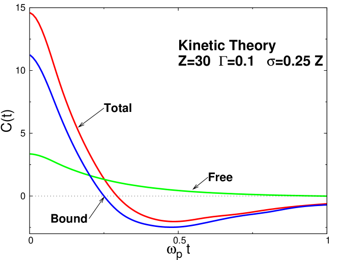
Figure 4: Bound and free state contributions to $C(t)$ for $Z=30$.

.

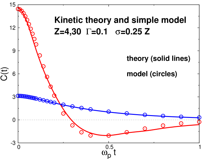
Figure 5: Comparison of $C(t)$ calculated from kinetic theory and from the simple model for $Z=4$ and $30$.

The results of this section demonstrate the utility of the kinetic theory for conditions of strong ion - electron coupling. Although only weak electron - electron coupling was considered, the theory is applicable to strong coupling among electrons as well. Also, while attention in this section has been limited to the electric field autocorrelation function it is clear that the analysis applies with equal ease to the dynamic structure factor as well, with only the additional complication of more parameters (i.e., two position vectors) characterizing that function. The decomposition of the correlation function into bound and free contributions demonstrates that the interesting features associated with increasing $Z$ can be attributed entirely to the increasing contribution from bound states.

V A simple, analytic, and accurate model

Consider again the electric field auto correlation function given by (30) explicitly decomposed into its bound and free contributions

$$C(t)=C^{b}(t)+C^{f}(t),$$ (32)

$$C^{b,f}(t)\rightarrow\int d\mathbf{r}d\mathbf{v}\left(n\left(r\right)\phi\left(v\right)\right)_{b,f}\mathbf{e}(\mathbf{r})\cdot e^{-\mathcal{L}_{0}t}\mathbf{e}_{s}(\mathbf{r}),$$ (33)

The objective here is to capture the qualitative features of the bound and free contributions in a very simple model that allows further elaboration of their relative roles and the mechanisms involved. This is accomplished by assuming circular trajectories for the bound states and straight line trajectories for the free states,

$$C^{f}(t)\rightarrow\int d\mathbf{r}d\mathbf{v}\left(n\left(r\right)\phi\left(v\right)\right)_{f}\mathbf{e}(\mathbf{r})\cdot\mathbf{e}_{s}(\mathbf{r-v}t),$$ (34)

$$C^{b}(t)\rightarrow\int d\mathbf{r}d\mathbf{v}\left(n\left(r\right)\phi\left(v\right)\right)_{b}e(r)e_{s}(r)\cos\left(\frac{v_{c}(r)}{r}t\right).$$ (35)

Here $\cos(v_{c}(r)t/r)=\widehat{\mathbf{r}}\cdot\widehat{\mathbf{r}}\left(t\right)$ and $r(t)=r$ for circular obits. In this case the velocity must be orthogonal to $\mathbf{r}$ with the specified magnitude

$$v_{c}\left(r\right)=\sqrt{\frac{r}{m}\frac{d\mathcal{V}_{ie}\left(r\right)}{dr}},$$ (36)

for consistency with Newton’s equations. The Maxwellian in $\left(n\left(r\right)\phi\left(v\right)\right)_{b}$ must therefore be replaced by this restriction on the velocities

$$\left(n\left(r\right)\phi\left(v\right)\right)_{b}\rightarrow\frac{1}{2\pi}n_{b}\left(r\right)\Theta\left(v_{m}(r)-v\right)\delta\left(\mathbf{v\cdot}\widehat{\mathbf{r}}\right)\delta\left(u-v_{c}\left(r\right)\right),$$ (37)

where $\mathbf{u}$ is the component of $\mathbf{v}$ orthogonal to $\mathbf{r}$. The factor $n_{b}(r)$ is given by (27) and is required by the correct normalization on integration over all velocities. Equation (35) then becomes

$$C^{b}(t)\rightarrow 4\pi\int_{0}^{\infty}drr^{2}n_{b}\left(r\right)e(r)e_{s}(r)\cos(\omega_{c}(r)t)$$ (38)

where $\omega_{c}(r)\equiv v_{c}(r)/r$. Note that these modifications of the trajectories do not affect the initial value, $C(0)$, which is still exact.

One further simplification is made to complete the  model. The effective potential $\mathcal{V}_{ie}\left(r\right)$ is replaced by its weak coupling Debye form

$$\mathcal{V}_{ie}\left(r\right)\rightarrow-\frac{\overline{Z}e^{2}}{\left(1-\left(\delta/\lambda\right)^{2}\right)}\frac{1}{r}\left(e^{-r/\lambda}-e^{-r/\delta}\right),$$ (39)

where $\lambda=r_{0}/\sqrt{3\Gamma}$ is the Debye length and $\delta$ is the quantum regularization length of (2). The corresponding electron density is now the non-linear Debye form

$$n\left(r\right)=n_{e}\exp\left(\beta\frac{\overline{Z}e^{2}}{\left(1-\left(\delta/\lambda\right)^{2}\right)}\frac{1}{r}\left(e^{-r/\lambda}-e^{-r/\delta}\right)\right).$$ (40)

This is exact in the weak coupling limit, with $\overline{Z}\rightarrow Z$. More generally, $\overline{Z}$ is chosen to give the correct value of $C(0)$ using (39) and (40) in the exact equation for $C(0)$ and adjusting $\overline{Z}$ to fit the values obtained from HNC

$$C^{\ast}(0)=\frac{r_{0}^{4}}{e^{2}}C(0)=\frac{3}{\overline{Z}\Gamma}\int_{0}^{\infty}dyye^{-y}\left(e^{\overline{Z}f(y)}-1\right),$$ (41)

with

$$f(y)=\frac{1}{y}\frac{\Gamma}{\delta^{\ast}\left(1-\left(\sqrt{3\Gamma}\delta^{\ast}\right)^{2}\right)}\left(e^{-\delta^{\ast}\sqrt{3\Gamma}y}-e^{-y}\right),\hskip 18.06749pt\delta^{\ast}=\frac{\delta}{r_{0}}.$$ (42)

Table 1 gives the values obtained using $C^{\ast}(0)$ from the HNC approximation, for the case $\Gamma=0.1$ and $\sigma=0.25Z$.

$Z$	$\overline{Z}$	$C^{\ast}(0)$
$1$	$1.03$	$2.67$
$4$	$3.76$	$3.13$
$8$	$7.29$	$3.92$
$20$	$16.79$	$8.15$
$30$	$22.87$	$14.4$
$40$	$27.20$	$22.7$

Table 1: Effective charge number $\overline{Z}$ for the Debye form

Figure 5 shows again the results of Figures 3 and 4 for $Z=4$ and $30$, now including as well the results from the simple model of this section. Remarkably, the use of the Debye form with the straight line and circular trajectories gives an accurate representation of the kinetic theory results. This provides the basis for a practical tool for use in more complex conditions, as discussed in the last section, and for other correlation functions, as illustrated in the next section.

VI Dielectric function

The last two sections addressed the short time form (29) of the correlation functions for which the dielectric function behaves as $\epsilon\left(\mathbf{r},\mathbf{r}^{\prime};z\right)\rightarrow\delta\left(\mathbf{r}-\mathbf{r}^{\prime}\right)$. For very long times (small $z$) $\epsilon\left(\mathbf{r},\mathbf{r}^{\prime};z\right)$ crosses over to represent static screening. At intermediate times there are contributions from collective excitations. Their description is more complex than for the uniform electron gas for which the space dependence of the dielectric function occurs only through $\mathbf{r}-\mathbf{r}^{\prime}$. To simplify the discussion here consider the weak electron - electron limit (but possibly strong ion - electron coupling) for which $\mathcal{V}_{ee}(\mathbf{r},\mathbf{r}^{\prime})\rightarrow\mathcal{V}_{ee}(\left|\mathbf{r}-\mathbf{r}^{\prime}\right|)$ and define the partial transform

$$\widetilde{\epsilon}\left(\mathbf{r},\mathbf{k};z\right) \equiv \int d\mathbf{r}^{\prime}e^{i\mathbf{k\cdot}\left(\mathbf{r}^{\prime}-\mathbf{r}\right)}\epsilon\left(\mathbf{r},\mathbf{r}^{\prime};z\right)$$ (43)

$$= 1+\beta n(r)\widetilde{V}_{ee}(k)\int_{0}^{\infty}dte^{-zt}\int d\mathbf{v}\phi\left(v\right)i\mathbf{k}\cdot\mathbf{v}\left(-t\right)e^{i\mathbf{k}\cdot\left(\mathbf{r}\left(-t\right)\mathbf{-r}\right)}.$$

Collective excitations for the non-uniform system, $z\left(\mathbf{k},\mathbf{r}\right)$, are defined by $\widetilde{\epsilon}\left(\mathbf{r},\mathbf{k};z\left(\mathbf{k},\mathbf{r}\right)\right)=0$. For zero charge number on the ion, $Z=0$, $\widetilde{\epsilon}\left(\mathbf{r},\mathbf{k};z\right)$ reduces to the familiar RPA dielectric function of the uniform electron gas

$$\widetilde{\epsilon}\left(\mathbf{r},\mathbf{k};z\right)\rightarrow\widetilde{\epsilon}_{RPA}\left(n_{e},\mathbf{k};z\right)=1+\beta n_{e}\widetilde{V}_{ee}(k)\int_{0}^{\infty}dte^{-zt}\int d\mathbf{v}\phi\left(v\right)i\mathbf{k}\cdot\mathbf{v}e^{-i\mathbf{k}\cdot\mathbf{v}t}$$ (44)

identifying the excitation spectrum $z\left(\mathbf{k}\right)$.

For $Z\neq 0$ the modes, $z\left(\mathbf{k},\mathbf{r}\right)$, depend on $\mathbf{r}$ due to the inhomogeneity caused by the ion. As an example, consider the solutions with very large $z$. Expanding $\widetilde{\epsilon}\left(\mathbf{r},\mathbf{k};z\right)$ to order $1/z^{2}$ gives

$$z^{2}\left(\mathbf{k},\mathbf{r}\right)=-\frac{n(r)\widetilde{V}_{ee}(k)k^{2}}{m}+ik_{\parallel}r\frac{n(r)\widetilde{V}_{ee}(k)}{m}\beta m\omega_{c}^{2}\left(r\right)+..,$$ (45)

where $k_{\parallel}=\mathbf{k}\cdot\mathbf{r/}r$ is the component of $\mathbf{k}$ along $\mathbf{r}$. For small $k$ the first term goes to the square of the local plasma frequency

$$\frac{n(r)k^{2}\widetilde{V}_{ee}(k)}{m}\rightarrow\frac{4\pi n(r)e^{2}}{m}\equiv\omega_{p}^{2}\left(r\right),$$ (46)

and (45) simplifies to

$$z^{2}\left(\mathbf{k},\mathbf{r}\right)=-\omega_{p}^{2}\left(r\right)+i\omega_{c}^{2}\left(r\right)\frac{k_{\parallel}r}{\left(k\lambda_{D}\left(r\right)\right)^{2}}+..,$$ (47)

Here $\lambda_{D}^{2}\left(r\right)=1/\beta m\omega_{p}^{2}\left(r\right)$ is the corresponding local Debye length. Therefore, if $k_{\parallel}=0$ the system supports plasmons with frequencies defined in terms of the local density. This is suggestive of a more general “local density approximation” Gunnarson where the dielectric function for the uniform electron gas is modified by replacing the uniform density with the actual non-uniform density

$$\widetilde{\epsilon}\left(\mathbf{r},\mathbf{k};z\right)\rightarrow\widetilde{\epsilon}_{RPA}\left(n_{e},\mathbf{k};z\right)\Big{|}_{n_{e}=n\left(r\right)}.$$ (48)

However, this is not correct in general as is evident from (45) for $k_{\parallel}\neq 0$ and the following.

To continue with the evaluation of (43) separate into bound and free contributions

$$\widetilde{\epsilon}\left(\mathbf{r},\mathbf{k};z\right) = 1+\beta n(r)\widetilde{\mathcal{V}}_{ee}(k)\int_{0}^{\infty}dte^{-zt}\frac{d}{dt}\left[\int d\mathbf{v}\phi\left(v\right)\Theta\left(v-v_{m}(r)\right)e^{i\mathbf{k}\cdot\left(\mathbf{r}\left(-t\right)\mathbf{-r}\right)}\right.$$ (49)

$$\left.+\frac{1}{2\pi}f_{b}(r)\int d\mathbf{v}\Theta\left(v_{m}(r)-v\right)\delta\left(\mathbf{v\cdot}\widehat{\mathbf{r}}\right)\delta\left(u-v_{c}\left(r\right)\right)e^{i\mathbf{k}\cdot\left(\mathbf{r}\left(-t\right)\mathbf{-r}\right)}\right].$$

Next, introduce the approximate trajectories of the last section. The analysis is straightforward but lengthy so only the final result is given here

$$\widetilde{\epsilon}\left(\mathbf{r},\mathbf{k};z\right)=1+\beta\widetilde{\mathcal{V}}_{ee}(k)\left(n_{f}(r)I_{f}(k,r,z)+n_{b}(r)I_{b}(\mathbf{k},\mathbf{r,}z)\right).$$ (50)

The first term of the brackets, proportional to $n_{f}(r)\equiv n(r)-n_{b}(r)$, is the contribution from free states, while the second term proportional to $n_{b}(r)$ is that from bound states (recall (27) for the bound state contribution $n_{b}(r)$). The functions $I_{f}(k,r,z)$ and $I_{b}(\mathbf{k},\mathbf{r,}z)$ are

$$I_{f}(k,r,z)=kv_{0}\int_{0}^{\infty}dte^{-zt}\frac{\int_{v_{m}(r)/v_{0}}^{\infty}dxx^{3}e^{-x^{2}}j_{1}\left(kv_{0}tx\right)}{\int_{v_{m}(r)/v_{0}}^{\infty}dxx^{2}e^{-x^{2}}},$$ (51)

$$I_{b}(\mathbf{k},\mathbf{r,}z) = \int_{0}^{\infty}dte^{-zt}e^{ik_{\parallel}r\left(\cos(\omega_{c}(r)t)-1\right)}\Bigg{[}-ik_{\parallel}v_{c}(r)\sin(\omega_{c}(r)t)J_{0}(k_{\perp}v_{c}\left(r\right)\sin(\omega_{c}(r)t))$$ (52)

$$\qquad\qquad\qquad\qquad\qquad\qquad\qquad\qquad+\ \frac{d}{dt}J_{0}(k_{\perp}v_{c}\left(r\right)\sin(\omega_{c}(r)t))\Bigg{]}.$$

The Bessel functions $j_{1}(x)$ and $J_{0}(x)$ are

$$j_{1}(x)=\frac{1}{x^{2}}\left(\sin x-x\cos x\right),\hskip 18.06749ptJ_{0}(x)=\frac{1}{2\pi}\int_{0}^{2\pi}d\phi e^{ix\cos\phi}.$$ (53)

The free state contribution depends only on the magnitudes $k,r$ while the bound state contribution depends on the directions as well, where $k_{\parallel}$ and $k_{\perp}$ are the components of $\mathbf{k}$ parallel and perpendicular to $\mathbf{r}$.

Consider the small $k$, long wavelength limit of this expression for $\widetilde{\epsilon}\left(\mathbf{r},\mathbf{k};z\right)$. Retaining the leading order contributions to (51) and (52) gives

$$\widetilde{\epsilon}\left(\mathbf{r},\mathbf{k};z\right) \rightarrow 1+\allowbreak\frac{\omega_{p}^{2}\left(r\right)}{z^{2}}\left(\frac{n_{f}(r)}{n(r)}+\frac{4}{3\sqrt{\pi}}\left(\frac{v_{m}(r)}{v_{0}}\right)^{3}e^{-\left(v_{m}(r)/v_{0}\right)^{2}}\right)$$ (54)

$$+\frac{\omega_{c}^{2}(r)}{z^{2}+\omega_{c}^{2}(r)}\frac{ik_{\parallel}r}{\left(k\lambda_{D}\left(r\right)\right)^{2}}\frac{n_{b}(r)}{n(r)}.$$

The limiting forms for these long wavelength excitations as functions of the ion charge number $Z$ are

$$z^{2}\rightarrow\left\{\begin{array}[]{c}-\omega_{p}^{2}\left(r\right),\hskip 18.06749ptZ<1\\ -\omega_{c}^{2}(r)\left(1+\frac{ik_{\parallel}r}{\left(k\lambda_{D}\left(r\right)\right)^{2}}\right),\hskip 18.06749ptZ>>1\end{array}\right.$$ (55)

The local plasmons are recovered for small charge numbers, while for large charge numbers the local circular frequencies $\omega_{c}^{2}(r)$ dominate. The complex coefficient in (55) implies that these excitations are damped.

The dielectric function $\widetilde{\epsilon}\left(\mathbf{r},\mathbf{k};z\right)$ is quite complex, but it is seen that the simple model of straight line and circular orbits simplifies this considerably. Further analysis of the collective modes for the inhomogeneous electron gas will be given elsewhere.

VII Discussion

A very general description of time correlation functions for electron properties near a positive ion has been given by the Markovian approximation (15). The time dependence has two contributions, an effective single particle dynamics that dominates for short and intermediate times, and a modification of that dynamics due to collective modes. The single particle dynamics has a strong dependence on the ion charge number $Z$, which is due to the growing dominance of bound states for large $Z$. The description is valid for such strong coupling conditions, since the Markovian approximation preserves the exact equilibrium electron - ion correlations in the effective potential governing the single particle dynamics. Similarly the electron - electron potential is renormalized by the exact equilibrium electron - electron correlations.

The description has been illustrated here for the special case of the electric field autocorrelation function under the same conditions as have been studied by MD simulations ilya . As the time scales are short, only the effective single particle dynamics has been considered. It remains to explore other correlation functions for which the collective modes are expected to be more important, and to provide a detailed characterization of those modes via the inhomogeneous electron gas dielectric function. The promise for progress in this direction is provided by the success of a simple model for the bound and free state dynamics.

There are several avenues for future directions based on this work:

1. The analysis here is based on a semi-classical description using a ”regularized” electron - ion potential. The quality of this type of description can be benchmarked by comparison with a corresponding quantum description of the same effective single particle dynamics.

2. A generalization of the Markovian approximation to a two component electron - ion plasma is straightforward. In that case the interest is in the electron dynamics in the vicinity of one of the ions. An additional feature is the effect of the dynamics of the ions. This constitutes a kinetic theory for the two particle (electron and ion) distribution function.

3. The spectral line shapes from charged radiators are an important diagnostic tool in laser fusion studies. A recent formulation of this problem including all plasma charge correlations is expressed in terms of constrained equilibrium time correlation functions wrighton . The constraint arises from a specified value of the total ion electric field during the dynamical broadening by the electrons. The simple model described here provides the potential for practical evaluation of these constrained time correlation functions under the demanding conditions of hot, dense matter. The role of charge correlations in plasma spectroscopy also has been discussed recently in reference 8.

4. A corresponding identification of the Markov limit in a fully quantum analysis is straightforward but the resulting renormalization of the ion - electron and electron - electron interactions by initial correlations is more complicated. Still, the structure obtained here of single electron dynamics in the presence of the ion modified by collective modes of the dielectric function remains the same.

5. The attractive distortion of the electron density by the ions, particularly for the bound states, is a type of electron confinement. The analysis here can be applied to real traps for charged particle confinement (e.g., dusty plasmas near an electrode, ultra-cold plasmas in a laser trap, valence electrons in metallic clusters, electrons in quantum dots). Significant differences include complete confinement and relaxing charge neutrality.

VIII Acknowledgements

The research was supported by the NSF/DOE Partnership in Basic Plasma Science and Engineering under the Department of Energy award DE-FG02-07ER54946.

Appendix A Equilibrium BBGKY hierarchy

Consider a point ion of charge number $Z$ in an electron gas of average density $n_{e}$ with a positive uniform neutralizing background of density $n_{b}=n_{e}$. The equilibrium structure of the electrons in the presence of the ion is given by the one and two particle distribution functions, defined for the equilibrium ensemble by

$$f_{ie}\left(r_{10},\mathbf{v}_{0},\mathbf{v}_{1}\right)\equiv N_{e}\int dx_{2}..dx_{N_{e}}\rho_{e}\left(\Gamma\right)$$ (56)

$$f_{iee}\left(\mathbf{r}_{10},\mathbf{r}_{20},\mathbf{v}_{0},\mathbf{v}_{1},\mathbf{v}_{2}\right)\equiv N_{e}^{2}\int dx_{3}..dx_{N_{e}}\rho_{e}\left(\Gamma\right)$$ (57)

where $\mathbf{r}_{10}=\mathbf{r}_{1}-\mathbf{r}_{0}$ is the position of an electron at $\mathbf{r}_{1}$ relative to the ion at $\mathbf{r}_{0}$. This position dependence reflects the fluid symmetry (rotational invariance) about the ion. The distribution function $f_{ie}\left(r_{10},\mathbf{v}_{0},\mathbf{v}_{1}\right)$ obeys the equilibrium BBGKY hierarchy equation

$$\left(\mathbf{v}_{1}\cdot\mathbf{\nabla}_{1}+\mathbf{v}_{0}\cdot\mathbf{\nabla}_{0}+m_{0}^{-1}\mathbf{F}_{ie}\left(\mathbf{r}_{10}\right)\cdot\mathbf{\nabla}_{\mathbf{v}_{0}}+m_{e}^{-1}\mathbf{F}_{ei}\left(\mathbf{r}_{10}\right)\cdot\mathbf{\nabla}_{\mathbf{v}_{1}}\right)f_{ie}\left(r_{10},\mathbf{v}_{0},\mathbf{v}_{1}\right)$$ (58)

$$= -\int d\mathbf{r}_{2}d\mathbf{v}_{2}\left(m_{0}^{-1}\mathbf{F}_{ie}\left(\mathbf{r}_{20}\right)\cdot\mathbf{\nabla}_{\mathbf{v}_{0}}+m_{e}^{-1}\mathbf{F}_{ee}\left(\mathbf{r}_{21}\right)\cdot\mathbf{\nabla}_{\mathbf{v}_{1}}\right)f_{iee}\left(\mathbf{r}_{10},,\mathbf{r}_{20},\mathbf{v}_{0},\mathbf{v}_{1},\mathbf{v}_{2}\right)$$

$$+\int d\mathbf{r}_{2}\left(m_{0}^{-1}\mathbf{F}_{ie}\left(\mathbf{r}_{20}\right)\cdot\mathbf{\nabla}_{\mathbf{v}_{0}}+m_{e}^{-1}\mathbf{F}_{ee}\left(\mathbf{r}_{21}\right)\cdot\mathbf{\nabla}_{\mathbf{v}_{1}}\right)f_{ie}\left(r_{10},\mathbf{v}_{0},\mathbf{v}_{1}\right)n_{b}.$$

The last term on the right side is due to the interaction of the ion and electron with the uniform neutralizing background whose density is $n_{b}=n_{e}$. Also, $\mathbf{F}_{ie}\left(\mathbf{r}_{10}\right)$ is the force of the electron on the ion, $\mathbf{F}_{ei}=-\mathbf{F}_{ie}$ is the reaction force of the ion on the electron, and $\mathbf{F}_{ee}\left(\mathbf{r}_{21}\right)$ is the force between electrons. These forces are derived from corresponding potentials

$$\mathbf{F}_{ei}=-\mathbf{F}_{ie}=-\mathbf{\nabla}_{1}V_{ei}\left(r_{10}\right),\hskip 18.06749pt\mathbf{F}_{ee}\left(\mathbf{r}_{21}\right)=-\mathbf{\nabla}_{1}V_{ee}\left(r_{21}\right).$$

The solutions to (58) have the forms

$$f_{ie}\left(\mathbf{r}_{0},\mathbf{v}_{0},\mathbf{r}_{1},\mathbf{v}_{1}\right)=\phi_{i}(v_{0})\phi_{e}(v_{1})n\left(r_{10}\right)$$ (59)

$$f_{iee}\left(\mathbf{r}_{0},\mathbf{v}_{0},\mathbf{r}_{1},\mathbf{v}_{1},\mathbf{r}_{2},\mathbf{v}_{2}\right)=\phi_{i}(v_{0})\phi_{e}(v_{1})\phi_{e}(v_{2})n\left(\mathbf{r}_{10},\mathbf{r}_{20}\right)$$ (60)

Here $\phi_{i}(v_{0})$ and $\phi_{e}(v_{1})$ are the Maxwellians for the ion and electron

$$\phi_{\alpha}\left(v\right)=\left(\frac{m_{\alpha}}{2\pi k_{B}T}\right)^{3/2}e^{-\frac{m_{\alpha}v^{2}}{2k_{B}T}},$$ (61)

and $n(r_{10}),$ $n(\mathbf{r}_{10},\mathbf{r}_{20})$ are the one and two particle electron number densities (relative to the ion) normalized to $N_{e}$ and $N_{e}^{2}$, respectively. Use of these forms in (58) gives directly

$$0 = \mathbf{v}_{0}\cdot\Bigg{(}-\mathbf{\nabla}_{1}n\left(r_{10}\right)-\beta n\left(r_{10}\right)\mathbf{\nabla}_{1}V_{ei}\left(r_{10}\right)$$ (62)

$$\qquad\qquad\qquad\qquad\qquad\qquad-\beta\int d\mathbf{r}_{2}\left[n\left(\mathbf{r}_{10},\mathbf{r}_{20}\right)-n\left(r_{10}\right)n_{e}\right]\mathbf{\nabla}_{2}V_{ei}\left(r_{20}\right)\Bigg{)}$$

$$+\,\mathbf{v}_{1}\cdot\Bigg{(}\mathbf{\nabla}_{1}n\left(r_{10}\right)+\beta n\left(r_{10}\right)\mathbf{\nabla}_{1}V_{ei}\left(r_{10}\right)$$

$$\qquad\qquad\qquad\qquad\qquad\qquad-\beta\int d\mathbf{r}_{2}\left[n\left(\mathbf{r}_{10},\mathbf{r}_{20}\right)-n\left(r_{10}\right)n_{e}\right]\mathbf{\nabla}_{2}V_{ee}\left(r_{21}\right)\Bigg{)}$$

Since the velocities of the ion and electron are independent, the following two equations hold

$$\mathbf{\nabla}_{1}\ln n\left(r_{10}\right)=-\beta\mathbf{\nabla}_{1}V_{ei}\left(r_{10}\right)-\beta n_{e}\int d\mathbf{r}_{2}\left[\frac{n\left(\mathbf{r}_{10},\mathbf{r}_{20}\right)}{n\left(r_{10}\right)n_{e}}-1\right]\mathbf{\nabla}_{2}V_{ei}\left(r_{20}\right)$$ (63)

$$\mathbf{\nabla}_{1}\ln n\left(r_{10}\right)=-\beta\mathbf{\nabla}_{1}V_{ei}\left(r_{10}\right)+\beta n_{e}\int d\mathbf{r}_{2}\left[\frac{n\left(\mathbf{r}_{10},\mathbf{r}_{20}\right)}{n\left(r_{10}\right)n_{e}}-1\right]\mathbf{\nabla}_{2}V_{ee}\left(r_{21}\right)$$ (64)

This provides two, seemingly independent, equations for the same electron density around the ion $n_{ie}\left(r_{10}\right)$. Their equivalence implies

$$\int d\mathbf{r}_{2}\left(\mathbf{F}_{ie}\left(r_{20}\right)+\mathbf{F}_{ee}\left(r_{12}\right)\right)\left[n_{ee}\left(\mathbf{r}_{10},\mathbf{r}_{20}\right)-n\left(r_{10}\right)n_{e}\right]=0$$ (65)

which means that the total external force on the system of two selected particles, the ion and the one electron, is zero at equilibrium. In other words, the distortion of $n_{iee}\left(\mathbf{r}_{10},\mathbf{r}_{20}\right)$ is just such as to enforce this condition. Both equations (63) and (64) are useful, as illustrated in the following two subsections.

In the remainder of the Appendices and in the text, only the special case of a massive ion fixed at the origin is considered.

A.1 Screened electric field

The electric field due to one electron at the ion is defined by

$$\mathbf{e}\left(\mathbf{r}\right)=\frac{1}{Ze}\nabla_{\mathbf{r}}V_{ei}\left(r\right).$$ (66)

The electric field autocorrelation function of (23) depends on the associated statically screened field

$$\mathbf{e}_{s}(\mathbf{r})=\int d\mathbf{r}^{\prime}\mathbf{e}(\mathbf{r}^{\prime})s\left(\mathbf{r}^{\prime},\mathbf{r}\right)=\mathbf{e}(\mathbf{r})+\frac{1}{n\left(r\right)}\int d\mathbf{r}^{\prime}\mathbf{e}(\mathbf{r}^{\prime})\left(n\left(\mathbf{r},\mathbf{r}^{\prime}\right)-n\left(r\right)n\left(r^{\prime}\right)\right).$$ (67)

This dependence on the two electron density $n\left(\mathbf{r},\mathbf{r}^{\prime}\right)$ can be eliminated using (63) to get

$$\mathbf{e}_{s}(\mathbf{r})=-\frac{1}{\beta Ze}\mathbf{\nabla}_{1}\ln n\left(r\right).$$ (68)

An effective potential is defined in terms of the density $n\left(r\right)$ in (11)

$$\mathcal{V}_{ie}\left(r\right)\equiv-\beta^{-1}\ln n\left(r\right),$$ (69)

so the screened electric field is given in terms of the gradient of this effective potential

$$\mathbf{e}_{s}(\mathbf{r})=\frac{1}{Ze}\mathbf{\nabla}_{1}\mathcal{V}_{ie}\left(r\right).$$ (70)

A.2 Hypernetted chain approximation

A simple and accurate method to determine the density is given by the hypernetted chain (HNC) integral equations hansen . They can be obtained from the usual form for a three component plasma of electrons, protons, and ions of charge number $Z$. Then the limit is taken of uniform proton distribution and dilute concentration for the ions of charge $Z$. Instead, it is useful here to state the result as an approximation to (64). Consider the mean field limit of no electron - electron correlations

$$\int d\mathbf{r}_{2}\left[\frac{n\left(\mathbf{r}_{1},\mathbf{r}_{2}\right)}{n\left(r_{1}\right)n_{e}}-1\right]\mathbf{\nabla}_{2}V_{ee}\left(r_{21}\right)\rightarrow\int d\mathbf{r}_{2}\left[\frac{n\left(r_{1}\right)n\left(r_{2}\right)}{n\left(r_{1}\right)n_{e}}-1\right]\mathbf{\nabla}_{2}V_{ee}\left(r_{21}\right).$$ (71)

Then equation (64) simplifies to

$$\mathbf{\nabla}_{1}\left[\ln n\left(r_{1}\right)+\beta V_{ei}\left(r_{1}\right)+\beta n_{e}\int d\mathbf{r}_{2}\left(\frac{n\left(r_{2}\right)}{n_{e}}-1\right)V_{ee}\left(r_{21}\right)\right]=0,$$ (72)

or

$$\ln\frac{n\left(r_{1}\right)}{n_{e}}=-\beta V_{ei}\left(r_{1}\right)-\beta n_{e}\int d\mathbf{r}_{2}\left(\frac{n\left(r_{2}\right)}{n_{e}}-1\right)V_{ee}\left(r_{21}\right).$$ (73)

An arbitrary constant has been used to assure the limit $n\left(r_{1}\right)\rightarrow n_{e}$ when $V_{ei}\left(r_{1}\right)\rightarrow 0$. Equation (73) is an integral form of the Boltzmann - Poisson equation.

The HNC approximation is similar, but retains electron - electron correlations in the absence of the ion

$$-\beta\int d\mathbf{r}_{2}\left[\frac{n\left(\mathbf{r}_{1},\mathbf{r}_{2}\right)}{n\left(r_{1}\right)n_{e}}-1\right]\mathbf{\nabla}_{2}V_{ee}\left(r_{21}\right)\rightarrow\int d\mathbf{r}_{2}\left[\frac{n\left(r_{1}\right)n\left(r_{2}\right)}{n\left(r_{1}\right)n_{e}}-1\right]\mathbf{\nabla}_{2}c_{ee}\left(r_{21}\right).$$ (74)

The function $c_{ee}\left(r_{21}\right)$ is the electron direct correlation function defined in terms of the electron - electron pair correlation function (without the ion), $n_{ee}\left(r_{21}\right)$, by the Ornstein - Zernicke equation

$$c_{ee}\left(r\right)=h_{ee}\left(r\right)-n_{e}\int d\mathbf{r}^{\prime}h_{ee}\left(r^{\prime}\right)c_{ee}\left(\left|\mathbf{r}-\mathbf{r}^{\prime}\right|\right),\hskip 18.06749pth_{ee}\left(r\right)=\frac{n_{ee}\left(r\right)}{n_{e}^{2}}-1$$ (75)

The approximation (74) in (64) gives the HNC approximation for $n\left(r\right)$

$$\ln\frac{n\left(r_{1}\right)}{n_{e}}=-\beta V_{ei}\left(r_{1}\right)+n_{e}\int d\mathbf{r}_{2}\left(\frac{n\left(r_{2}\right)}{n_{e}}-1\right)c_{ee}\left(r_{21}\right).$$ (76)

This is the same as (73) except that $V_{ee}\left(r_{21}\right)$ has been replaced by $-\beta^{-1}c_{ee}\left(r_{21}\right)$.

The electron - electron direct correlation function is determined independently from the Ornstein - Zernicke equation (75) and the HNC approximation

$$\ln\frac{n_{ee}\left(r\right)}{n_{e}^{2}}=-\beta V_{ee}\left(r_{1}\right)+h_{ee}\left(r\right)-c_{ee}\left(r\right).$$ (77)

Equations (75) - (77) are the HNC equations used for the numerical calculations presented here.

Appendix B Evaluation of $\mathcal{L}(x,x^{\prime};t=0)$

The dynamics of $C_{AB}(t)$ is conveniently expressed in terms of the fundamental correlation function $G(x,x^{\prime};t)$

$$C_{AB}(t)=\int dxdx^{\prime}a(x)G(x,x^{\prime};t)b(x^{\prime}),$$ (78)

$$G(x,x^{\prime};t)=\left\langle f\left(x,t\right)\left(f\left(x^{\prime}\right)-\left\langle f\left(x^{\prime}\right)\right\rangle\right)\right\rangle,\hskip 21.68121ptf\left(x\right)=\sum_{\alpha=1}^{N_{e}}\delta\left(x-x_{\alpha}\right).$$ (79)

The initial value $G(x,x^{\prime};0)$ is easily calculated, with the result

$$G(x,x^{\prime};0)=n\left(r\right)\phi\left(v\right)\left(\delta\left(x-x^{\prime}\right)+\phi\left(v^{\prime}\right)n\left(r^{\prime}\right)h\left(\mathbf{r},\mathbf{r}^{\prime}\right)\right).$$ (80)

In the last equality the two electron correlation function $h\left(\mathbf{r},\mathbf{r}^{\prime}\right)$ has been identified from (7). Comparison with (6) shows that $\overline{b}(x)$ can be written

$$\overline{b}(x)=\frac{1}{n(r)\phi(v)}\int dxG(x,x^{\prime};0)b\left(x^{\prime}\right).$$ (81)

This leads to the representation (5) for $C_{AB}(t)$

$$C_{AB}(t)=\int dxn(r)\phi\left(v\right)a(x)\overline{b}(x,t),$$ (82)

with

$$\overline{b}(x,t)=\int dx^{\prime}U\left(x,x^{\prime};t\right)\overline{b}(x^{\prime}),$$ (83)

$$U\left(x,x^{\prime};t\right)=\frac{1}{n(r)\phi(v)}\int dx^{\prime\prime}G(x,x^{\prime\prime};t)G^{-1}(x^{\prime\prime},x^{\prime};0)n(r^{\prime})\phi(v^{\prime}).$$ (84)

The inverse of $G(x,x^{\prime};0)$ has been introduced by the definition

$$\delta\left(x-x^{\prime}\right)=\int dx^{\prime\prime}G(x,x^{\prime\prime};0)G^{-1}(x^{\prime\prime},x^{\prime};0.)$$ (85)

It is verified that

$$G^{-1}(x,x^{\prime};0)=\frac{1}{n\left(r\right)\phi\left(v\right)}\delta\left(x-x^{\prime}\right)-c\left(\mathbf{r},\mathbf{r}^{\prime}\right),$$ (86)

if $c\left(\mathbf{r},\mathbf{r}^{\prime}\right)$ obeys the equation

$$c\left(\mathbf{r},\mathbf{r}^{\prime}\right)=h\left(\mathbf{r},\mathbf{r}^{\prime}\right)-\int d\mathbf{r}^{\prime\prime}h\left(\mathbf{r},\mathbf{r}^{\prime\prime}\right)n\left(\mathbf{r}^{\prime\prime}\right)c\left(\mathbf{r}^{\prime\prime},\mathbf{r}^{\prime}\right)$$ (87)

which is a generalization of the Ornstein-Zernicke equation hansen .

The formal equation for $\overline{b}(x,t)$, (8), follows from differentiation of (83) with respect to time and the identification

$$\mathcal{L}(x,x^{\prime};t)=-\int dx^{\prime\prime}\left(\partial_{t}U(x,x^{\prime\prime};t)\right)U^{-1}(x^{\prime\prime},x^{\prime};t).$$ (88)

This provides the desired result for identifying the Markovian approximation

$$\mathcal{L}\left(x,x^{\prime}\right)\equiv\mathcal{L}\left(x,x^{\prime};t=0\right)=-\partial_{t}U(x,x^{\prime};0),$$ (89)

where the property $U\left(x,x^{\prime};t=0\right)=\delta\left(x-x^{\prime}\right)$ has been used. Equation (84) gives finally

$$\mathcal{L}(x,x^{\prime})=-\,\frac{1}{n(r)\phi(v)}\int dx^{\prime\prime}\partial_{t}G(x,x^{\prime\prime};t)\Big{|}_{t=0}G^{-1}(x^{\prime\prime},x^{\prime};0)n(r^{\prime})\phi(v^{\prime}).$$ (90)

It only remains to calculate the initial derivative $\partial_{t}G(x,x^{\prime\prime};t)\mid_{t=0}$ to determine $\mathcal{L}(x,x^{\prime})$. To simplify the notation it is useful to denote the force on the electron due to both the ion and the uniform positive background by $\mathbf{F}_{0}\left(\mathbf{r}\right)$

$$\partial_{t}G(x,x^{\prime};t)\Big{|}_{t=0} = -\int dx_{1}\delta\left(x_{1}-x\right)\left(\mathbf{v}_{1}\cdot\nabla_{\mathbf{r}_{1}}+m^{-1}\mathbf{F}_{0}\left(\mathbf{r}_{1}\right)\cdot\nabla_{\mathbf{v}_{1}}\right)\Bigg{[}\delta\left(x_{1}-x^{\prime}\right)n\left(r_{1}\right)\phi\left(v_{1}\right)$$ (91)

$$\qquad\qquad+\int dx_{2}\delta\left(x_{2}-x^{\prime}\right)\phi\left(v_{1}\right)\phi\left(v_{2}\right)\left(n\left(\mathbf{r}_{1},\mathbf{r}_{2}\right)-n\left(r_{1}\right)n\left(r_{2}\right)\right)\Bigg{]}$$

$$-\int dx_{1}dx_{2}\delta\left(x_{1}-x\right)m^{-1}\mathbf{F}_{ee}\left(\mathbf{r}_{12}\right)\cdot\nabla_{\mathbf{v}_{1}}$$

$$\quad\times\Bigg{[}\left(\delta\left(x^{\prime}-x_{1}\right)+\delta\left(x^{\prime}-x_{2}\right)\right)\phi\left(v_{1}\right)\phi\left(v_{2}\right)n\left(\mathbf{r}_{1},\mathbf{r}_{2}\right)$$

$$\quad+\int dx_{3}\delta\left(x^{\prime}-x_{3}\right)\phi\left(v_{1}\right)\phi\left(v_{2}\right)\phi\left(v_{3}\right)\left(n\left(\mathbf{r}_{1},\mathbf{r}_{2},\mathbf{r}_{3}\right)-n\left(\mathbf{r}_{1},\mathbf{r}_{2}\right)n\left(r^{\prime}\right)\right)\Bigg{]}$$

$$= -\left(\mathbf{v}\cdot\nabla_{\mathbf{r}}+m^{-1}\mathbf{F}_{0}\left(\mathbf{r}\right)\cdot\nabla_{\mathbf{v}}\right)G(x,x^{\prime};0)$$

$$\ -\nabla_{\mathbf{v}}\cdot\delta\left(x^{\prime}-x\right)\phi\left(v\right)m^{-1}\int d\mathbf{r}_{2}\mathbf{F}_{ee}\left(\left|\mathbf{r}-\mathbf{r}_{2}\right|\right)n\left(\mathbf{r},\mathbf{r}_{2}\right)$$

$$\quad+\beta\phi\left(v\right)\phi\left(v^{\prime}\right)\mathbf{v}\cdot\Bigg{[}\mathbf{F}_{ee}\left(\left|\mathbf{r}-\mathbf{r}^{\prime}\right|\right)n\left(\mathbf{r},\mathbf{r}^{\prime}\right)$$

$$\qquad\qquad\quad+\int d\mathbf{r}_{2}\mathbf{F}_{ee}\left(\left|\mathbf{r}-\mathbf{r}_{2}\right|\right)\left(n\left(\mathbf{r}_{1},\mathbf{r}_{2},\mathbf{r}^{\prime}\right)-n\left(\mathbf{r}_{1},\mathbf{r}_{2}\right)n\left(r^{\prime}\right)\right)\Bigg{]}$$

The two integrals on the right can be performed using the hierarchy equation (64) for $n\left(r\right)$ and the corresponding next order hierarchy equation for $n\left(\mathbf{r}_{1},\mathbf{r}_{2}\right)$. In the current notation these are

$$\int d\mathbf{r}_{2}\mathbf{F}_{ee}\left(\left|\mathbf{r}-\mathbf{r}_{2}\right|\right)n\left(\mathbf{r},\mathbf{r}_{2}\right)=\beta^{-1}\mathbf{\nabla}_{1}n\left(r_{10}\right)-n\left(r_{10}\right)\mathbf{F}_{0}\left(\mathbf{r}\right),$$ (92)

$$\int d\mathbf{r}_{2}\mathbf{F}_{ee}\left(\left|\mathbf{r}-\mathbf{r}_{2}\right|\right)n\left(\mathbf{r}_{1},\mathbf{r}_{2},\mathbf{r}^{\prime}\right)=\beta^{-1}\mathbf{\nabla}_{1}n\left(\mathbf{r}_{1},\mathbf{r}^{\prime}\right)-\left(\mathbf{F}_{0}\left(\mathbf{r}_{1}\right)+\mathbf{F}_{ee}\left(\mathbf{r}_{1}-\mathbf{r}^{\prime}\right)\right)n\left(\mathbf{r}_{1},\mathbf{r}^{\prime}\right).$$ (93)

Then (74) becomes

$$\partial_{t}G(x,x^{\prime};t)\Big{|}_{t=0} = -\left(\mathbf{v}\cdot\nabla_{\mathbf{r}}+m^{-1}\mathbf{F}_{0}\left(r\right)\cdot\nabla_{\mathbf{v}}\right)G(x,x^{\prime};0)$$ (94)

$$-\left(m^{-1}\left(\beta^{-1}\nabla_{\mathbf{q}}\ln n\left(r\right)\right)-m^{-1}\mathbf{F}_{0}\left(r\right)\right)\cdot\nabla_{\mathbf{v}}\delta\left(x^{\prime}-x\right)n\left(r\right)\phi\left(v\right)$$

$$+\beta\phi\left(v\right)\phi\left(v^{\prime}\right)\left(n\left(\mathbf{r}_{1},\mathbf{r}_{2}\right)-n\left(r_{1}\right)n\left(r_{2}\right)\right)\mathbf{v}\cdot$$

$$\qquad\times\left(\beta^{-1}\nabla_{\mathbf{r}}\ln\left(n\left(\mathbf{r}_{1},\mathbf{r}_{2}\right)-n\left({r}_{1}\right)n\left({r}_{2}\right)\right)-\mathbf{F}_{0}\left(r\right)\right).$$

Next, eliminate the delta function using (80)

$$\partial_{t}G(x,x^{\prime};t)\Big{|}_{t=0} = -\left(\mathbf{v}\cdot\nabla_{\mathbf{r}}+m^{-1}\mathbf{F}_{0}\left(r\right)\cdot\nabla_{\mathbf{v}}\right)G(x,x^{\prime};0)$$ (95)

$$-\left(m^{-1}\left(\beta^{-1}\nabla_{\mathbf{r}}\ln n\left(r\right)\right)-m^{-1}\mathbf{F}_{0}\left(r\right)\right)\cdot\nabla_{\mathbf{v}}G(x,x^{\prime};0)$$

$$+\left(m^{-1}\left(\beta^{-1}\nabla_{\mathbf{r}}\ln n\left(r\right)\right)-m^{-1}\mathbf{F}_{0}\left(r\right)\right)$$

$$\qquad\qquad\cdot\nabla_{\mathbf{v}}\phi\left(v\right)\phi\left(v^{\prime}\right)\left(n\left(\mathbf{r},\mathbf{r}^{\prime}\right)-n\left(r\right)n\left(r^{\prime}\right)\right)$$

$$+\beta\phi\left(v\right)\phi\left(v^{\prime}\right)\left(n\left(\mathbf{r}_{1},\mathbf{r}_{2}\right)-n\left(r_{1}\right)n\left(r_{2}\right)\right)\mathbf{v}\cdot$$

$$\qquad\qquad\times\left(\beta^{-1}\nabla_{\mathbf{r}}\ln\left(n\left(\mathbf{r}_{1},\mathbf{r}_{2}\right)-n\left(r_{1}\right)n\left(r_{2}\right)\right)-\mathbf{F}_{0}\left(r\right)\right)$$

$$= -\left(\mathbf{v}\cdot\nabla_{\mathbf{r}}+m^{-1}\left(\beta^{-1}\nabla_{\mathbf{r}}\ln n\left(r\right)\right)\cdot\nabla_{\mathbf{v}}\right)G(x,x^{\prime};0)$$

$$\qquad+\phi\left(v\right)\phi\left(v^{\prime}\right)n\left(r\right)n\left(r^{\prime}\right)\mathbf{v}\cdot\nabla_{\mathbf{r}}h\left(\mathbf{r},\mathbf{r}^{\prime}\right).$$

Substitution of this result into (90) gives the generator for initial dynamics

$$\mathcal{L}(x,x^{\prime}) = \left(\mathbf{v}\cdot\nabla_{\mathbf{r}}+m^{-1}\left(\beta^{-1}\nabla_{\mathbf{r}}\ln n\left(\mathbf{r}\right)\right)\cdot\nabla_{\mathbf{v}}\right)\delta\left(x-x^{\prime}\right)$$ (96)

$$-\mathbf{v}\cdot\nabla_{\mathbf{r}}\int dx^{\prime\prime}\phi\left(v^{\prime\prime}\right)n\left(r^{\prime\prime}\right)h\left(\mathbf{r},\mathbf{r}^{\prime\prime}\right)G^{-1}(x^{\prime\prime},x^{\prime};0)\phi\left(v^{\prime}\right)n\left(r^{\prime}\right)$$

$$= \left(\mathbf{v}\cdot\nabla_{\mathbf{r}}+m^{-1}\left(\beta^{-1}\nabla_{\mathbf{r}}\ln n\left(r\right)\right)\cdot\nabla_{\mathbf{v}}\right)\delta\left(x-x^{\prime}\right)$$

$$-\mathbf{v}\cdot\nabla_{\mathbf{r}}\left[h\left(\mathbf{r},\mathbf{r}^{\prime}\right)-\int d\mathbf{r}^{\prime\prime}n\left(r^{\prime\prime}\right)h\left(\mathbf{r},\mathbf{r}^{\prime\prime}\right)c\left(\mathbf{r}^{\prime\prime},\mathbf{r}^{\prime}\right)\right]\phi\left(v^{\prime}\right)n\left(r^{\prime}\right).$$

Finally, using (87) the result (10) is obtained

$$\mathcal{L}(x,x^{\prime})=\left(\mathbf{v}\cdot\nabla_{\mathbf{r}}+m^{-1}\left(\beta^{-1}\nabla_{\mathbf{r}}\ln n\left(r\right)\right)\cdot\nabla_{\mathbf{v}}\right)\delta\left(x-x^{\prime}\right)-\mathbf{v}\cdot\nabla_{\mathbf{r}}c\left(\mathbf{r},\mathbf{r}^{\prime}\right)\phi\left(v^{\prime}\right)n\left(r^{\prime}\right).$$ (97)

Appendix C Solution to kinetic equation

The solution to (13) can be obtained in terms of an effective single electron dynamics by direct integration

$$\overline{b}(x,t)=e^{-\mathcal{L}_{0}t}\overline{b}(x)-\int_{0}^{t}d\tau e^{-\mathcal{L}_{0}\left(t-\tau\right)}\mathbf{v}\cdot\mathbf{\nabla}_{\mathbf{r}}\int d\mathbf{r}^{\prime}\beta\mathcal{V}_{ee}\left(\mathbf{r},\mathbf{r}^{\prime}\right)I(\mathbf{r}^{\prime},\tau),$$ (98)

where the generator for the effective single particle dynamics is

$$\mathcal{L}_{0}\equiv\mathbf{v}\cdot\nabla_{\mathbf{r}}-m^{-1}\nabla_{\mathbf{r}}\mathcal{V}_{ie}\left(r\right)\cdot\nabla_{\mathbf{v}},$$ (99)

and the source term $I(\mathbf{r},t)$ is

$$I(\mathbf{r},t)\equiv\int d\mathbf{v}\phi\left(v\right)n\left(r\right)\overline{b}(x,t).$$ (100)

The initial condition $\overline{b}(x)$ is given by (6). It is convenient at this point to introduce the corresponding Laplace transform

$$\widetilde{b}(x,z)=\int_{0}^{\infty}dte^{-zt}\overline{b}(x,t).$$ (101)

Then Laplace transformation of (98) gives the equation $\widetilde{b}(x,z)$

$$\widetilde{b}(x,z)=\mathcal{G}_{0}\overline{b}(x)-\mathcal{G}_{0}\mathbf{v}\cdot\mathbf{\nabla}_{\mathbf{r}}\int d\mathbf{r}^{\prime}\beta\mathcal{V}_{ee}\left(\mathbf{r},\mathbf{r}^{\prime}\right)\widetilde{I}(\mathbf{r}^{\prime},z),$$ (102)

$$\widetilde{I}(\mathbf{r},z)=\int d\mathbf{v}\phi\left(v\right)n\left(r\right)\widetilde{b}(x,z),\hskip 14.45377pt\mathcal{G}_{0}=\left(z+\mathcal{L}_{0}\right)^{-1}$$ (103)

An equation for $\widetilde{I}(\mathbf{r},z)$ follows from substitution of (102) into (103)

$$\widetilde{I}(\mathbf{r},z) = \int d\mathbf{v}\phi\left(v\right)n\left(r\right)\mathcal{G}_{0}\overline{b}(x,0)-\int d\mathbf{v}\phi\left(v\right)n(r)\mathcal{G}_{0}\mathbf{v}\cdot\mathbf{\nabla}_{\mathbf{r}}\int d\mathbf{r}^{\prime}\beta\mathcal{V}_{ee}\left(\mathbf{r},\mathbf{r}^{\prime}\right)\widetilde{I}(\mathbf{r}^{\prime},z)$$ (104)

$$= \widetilde{I}_{0}(\mathbf{r},z)+\int d\mathbf{r}^{\prime\prime}\pi\left(\mathbf{r},\mathbf{r}^{\prime\prime};z\right)\int d\mathbf{r}^{\prime}\mathcal{V}_{ee}\left(\mathbf{r}^{\prime\prime},\mathbf{r}^{\prime}\right)\widetilde{I}(\mathbf{r}^{\prime},z)$$

where $\pi\left(\mathbf{r},\mathbf{r}^{\prime\prime};z\right)$ is

$$\pi\left(\mathbf{r},\mathbf{r}^{\prime\prime};z\right)\equiv-\beta n(r)\int d\mathbf{v}\phi\left(v\right)\mathcal{G}_{0}\mathbf{v}\cdot\mathbf{\nabla}_{\mathbf{r}}\delta\left(\mathbf{r}-\mathbf{r}^{\prime\prime}\right),$$ (105)

and

$$\widetilde{I}_{0}(\mathbf{r},z)\equiv n\left(r\right)\int d\mathbf{v}\phi\left(v\right)\mathcal{G}_{0}\overline{b}(x).$$ (106)

This is an integral equation for $I(\mathbf{r},t)$ which can be written

$$\int d\mathbf{r}^{\prime}\epsilon\left(\mathbf{r},\mathbf{r}^{\prime};z\right)\widetilde{I}(\mathbf{r}^{\prime},z)=\widetilde{I}_{0}(\mathbf{r},z)$$ (107)

The dielectric function $\epsilon\left(\mathbf{r},\mathbf{r}^{\prime};z\right)$ is defined by

$$\epsilon\left(\mathbf{r},\mathbf{r}^{\prime};z\right)=\delta\left(\mathbf{r}-\mathbf{r}^{\prime}\right)-\int d\mathbf{r}^{\prime\prime}\pi\left(\mathbf{r},\mathbf{r}^{\prime\prime};z\right)\mathcal{V}_{ee}(\mathbf{r}^{\prime\prime},\mathbf{r}^{\prime}).$$ (108)

With these results (102) becomes

$$\widetilde{b}(x,z)=\mathcal{G}_{0}\left[\overline{b}(x)-\mathbf{v}\cdot\mathbf{\nabla}_{\mathbf{r}}\int d\mathbf{r}^{\prime\prime}\beta\mathcal{V}_{ee}\left(\mathbf{r},\mathbf{r}^{\prime\prime}\right)\int d\mathbf{r}^{\prime}\epsilon^{-1}\left(\mathbf{r}^{\prime\prime},\mathbf{r}^{\prime};z\right)\widetilde{I}_{0}(\mathbf{r}^{\prime},z)\right].$$ (109)

The inverse dielectric function is defined by

$$\int d\mathbf{r}^{\prime\prime}\epsilon\left(\mathbf{r},\mathbf{r}^{\prime\prime};z\right)\epsilon^{-1}\left(\mathbf{r}^{\prime\prime},\mathbf{r}^{\prime};z\right)=\delta\left(\mathbf{r}-\mathbf{r}^{\prime}\right)=\int d\mathbf{r}^{\prime\prime}\epsilon^{-1}\left(\mathbf{r},\mathbf{r}^{\prime\prime};z\right)\epsilon\left(\mathbf{r}^{\prime\prime},\mathbf{r}^{\prime};z\right).$$ (110)

Equation (109) is the desired solution to the kinetic equation, in terms of the single particle dynamics of $\mathcal{G}_{0}$, since all terms on the right side are now explicit.

The low frequency limit $\left(z=0\right)$ of $\epsilon\left(\mathbf{r},\mathbf{r}^{\prime};z\right)$ has a simple form in terms of the electron correlations. First write $\epsilon\left(\mathbf{r},\mathbf{r}^{\prime};z\right)$ as

$$\epsilon\left(\mathbf{r},\mathbf{r}^{\prime};z\right) = \delta\left(\mathbf{r}-\mathbf{r}^{\prime}\right)-\int d\mathbf{r}^{\prime\prime}\pi\left(\mathbf{r},\mathbf{r}^{\prime\prime};z\right)\mathcal{V}_{ee}(\mathbf{r}^{\prime\prime},\mathbf{r}^{\prime})$$ (111)

$$= \delta\left(\mathbf{r}-\mathbf{r}^{\prime}\right)+\beta n(r)\int d\mathbf{v}\phi\left(v\right)\mathcal{G}_{0}\left(\mathcal{G}_{0}^{-1}-z\right)\mathcal{V}_{ee}(\mathbf{r},\mathbf{r}^{\prime})$$

$$= \delta\left(\mathbf{r}-\mathbf{r}^{\prime}\right)+\beta n(r)\left(\mathcal{V}_{ee}(\mathbf{r},\mathbf{r}^{\prime})-z\int d\mathbf{v}\phi\left(v\right)\mathcal{G}_{0}\mathcal{V}_{ee}(\mathbf{r},\mathbf{r}^{\prime})\right).$$

where the definition of $\pi\left(\mathbf{r},\mathbf{r}^{\prime};z\right)$ in (105) and $\mathcal{G}_{0}$ in (103) have been used. Then taking the real and imaginary parts of $z$ going to zero gives

$$\epsilon\left(\mathbf{r},\mathbf{r}^{\prime};z=0\right)=\delta\left(\mathbf{r}-\mathbf{r}^{\prime}\right)+\beta n(r)\mathcal{V}_{ee}(\mathbf{r},\mathbf{r}^{\prime})=\delta\left(\mathbf{r}-\mathbf{r}^{\prime}\right)-n(r)c\left(\mathbf{r},\mathbf{r}^{\prime}\right).$$ (112)

It follows from the generalized Ornstein-Zernicke equation (87) that the inverse of $\epsilon\left(\mathbf{r},\mathbf{r}^{\prime};z=0\right)$ is

$$\epsilon^{-1}\left(\mathbf{r},\mathbf{r}^{\prime};z=0\right)=s\left(\mathbf{r}^{\prime},\mathbf{r}\right),$$ (113)

where the static structure factor is defined by

$$s\left(\mathbf{r},\mathbf{r}^{\prime}\right)=\delta\left(\mathbf{r}-\mathbf{r}^{\prime}\right)+h\left(\mathbf{r},\mathbf{r}^{\prime}\right)n\left(r^{\prime}\right)=\delta\left(\mathbf{r}-\mathbf{r}^{\prime}\right)+h\left(\mathbf{r}^{\prime},\mathbf{r}\right)n\left(r\right).$$ (114)

The high frequency limit $\left(z\rightarrow\infty\right)$ of $\epsilon\left(\mathbf{r},\mathbf{r}^{\prime};z\right)$ also has a simple form

$$\epsilon\left(\mathbf{r},\mathbf{r}^{\prime};z\right)\rightarrow\delta\left(\mathbf{r}-\mathbf{r}^{\prime}\right)+\frac{1}{z}\beta n(r)\int d\mathbf{v}\phi\left(v\right)\mathbf{v}\cdot\nabla_{\mathbf{r}}\mathcal{V}_{ee}(\mathbf{r},\mathbf{r}^{\prime})=\delta\left(\mathbf{r}-\mathbf{r}^{\prime}\right)$$ (115)

This implies no screening at asymptotically short times.

Appendix D Correlation functions

The Laplace transform of the correlation function (5) is

$$\widetilde{C}_{AB}(z)=\int dxn(r)\phi\left(v\right)a(x)\widetilde{b}(x,z).$$ (116)

Substitution of the solution (109) gives

$$\widetilde{C}_{AB}(z)=\int dxn(r)\phi\left(v\right)a(x)\mathcal{G}_{0}\left[\overline{b}(x)-\mathbf{v}\cdot\mathbf{\nabla}_{\mathbf{r}}\int d\mathbf{r}^{\prime\prime}\beta\mathcal{V}_{ee}\left(\mathbf{r},\mathbf{r}^{\prime\prime}\right)\int d\mathbf{r}^{\prime}\epsilon^{-1}\left(\mathbf{r}^{\prime\prime},\mathbf{r}^{\prime};z\right)\widetilde{I}_{0}(\mathbf{r}^{\prime},z)\right].$$ (117)

Considerable simplification occurs for the special case where $a(x)=a(\mathbf{r})$, i.e. it is independent of the velocity,

$$\widetilde{C}_{AB}(z) = \int dxn(r)\phi\left(v\right)a(\mathbf{r})\mathcal{G}_{0}\overline{b}(x)-\Bigg{[}\int d\mathbf{r}a(\mathbf{r})\beta n(r)\int d\mathbf{r}^{\prime\prime\prime}\int d\mathbf{v}\phi\left(v\right)\mathcal{G}_{0}\mathbf{v}\cdot\mathbf{\nabla}_{\mathbf{r}}\delta\left(\mathbf{r}-\mathbf{r}^{\prime\prime\prime}\right)$$

$$\times\int d\mathbf{r}^{\prime\prime}\mathcal{V}_{ee}\left(\mathbf{r}^{\prime\prime\prime},\mathbf{r}^{\prime\prime}\right)\int d\mathbf{r}^{\prime}\epsilon^{-1}\left(\mathbf{r}^{\prime\prime},\mathbf{r}^{\prime};z\right)\widetilde{I}_{0}(\mathbf{r}^{\prime},z)\Bigg{]}$$

$$= \int dxn(r)\phi\left(v\right)a(\mathbf{r})\mathcal{G}_{0}\overline{b}(x)+\int d\mathbf{r}a(\mathbf{r})\int d\mathbf{r}^{\prime\prime\prime}\pi\left(\mathbf{r},\mathbf{r}^{\prime\prime\prime};z\right)$$ (118)

$$\times\int d\mathbf{r}^{\prime\prime}\mathcal{V}_{ee}\left(\mathbf{r}^{\prime\prime\prime},\mathbf{r}^{\prime\prime}\right)\int d\mathbf{r}^{\prime}\epsilon^{-1}\left(\mathbf{r}^{\prime\prime},\mathbf{r}^{\prime};z\right)\widetilde{I}_{0}(\mathbf{r}^{\prime},z).$$

where use has been made of the definition (105) for $\pi\left(\mathbf{r},\mathbf{r}^{\prime\prime\prime};z\right)$. It follows from (108) that

$$\int d\mathbf{r}^{\prime\prime\prime}\pi\left(\mathbf{r},\mathbf{r}^{\prime\prime\prime};z\right)\int d\mathbf{r}^{\prime\prime}\mathcal{V}_{ee}\left(\mathbf{r}^{\prime\prime\prime},\mathbf{r}^{\prime\prime}\right)\epsilon^{-1}\left(\mathbf{r}^{\prime\prime},\mathbf{r}^{\prime};z\right)=\epsilon^{-1}\left(\mathbf{r},\mathbf{r}^{\prime};z\right)-\delta\left(\mathbf{r}-\mathbf{r}^{\prime}\right),$$ (119)

so (118) becomes

$$\widetilde{C}_{AB}(z)=\int dxn(r)\phi\left(v\right)a(\mathbf{r})\mathcal{G}_{0}\overline{b}(x)+\int d\mathbf{r}a(\mathbf{r})\int d\mathbf{r}^{\prime}\left[\epsilon^{-1}\left(\mathbf{r},\mathbf{r}^{\prime};z\right)-\delta\left(\mathbf{r}-\mathbf{r}^{\prime}\right)\right]\widetilde{I}_{0}(\mathbf{r}^{\prime},z)$$

$$=\int d\mathbf{r}\int d\mathbf{v}n\left(r\right)\phi\left(v\right)\int d\mathbf{r}^{\prime}a(\mathbf{r}^{\prime})\epsilon^{-1}\left(\mathbf{r}^{\prime},\mathbf{r};z\right)\mathcal{G}_{0}\overline{b}(x)$$ (120)

where (106) for $\widetilde{I}_{0}(\mathbf{r}^{\prime},z)$ has been made explicit, and the dummy labels $\mathbf{r},\mathbf{r}^{\prime}$ have been interchanged. Finally, this can be put in the simple form

$$\widetilde{C}_{AB}(z)=\int d\mathbf{r}d\mathbf{v}n\left(r\right)\phi\left(v\right)a_{s}(\mathbf{r};z)\mathcal{G}_{0}\overline{b}(x),$$ (121)

where

$$a_{s}(\mathbf{r};z)=\int d\mathbf{r}^{\prime}a(\mathbf{r}^{\prime})\epsilon^{-1}\left(\mathbf{r}^{\prime},\mathbf{r};z\right)$$ (122)

Use has been made of the fact that $n\left(r\right)\phi\left(v\right)$ commutes with $\mathcal{L}_{0}$.

D.1 Dynamic structure factor and field autocorrelation function

The dynamic structure factor is the autocorrelation function for the electron density, corresponding to

$$a(x)=\delta\left(\mathbf{r}-\mathbf{q}\right),\hskip 18.06749ptb(x)=\delta\left(\mathbf{r}-\mathbf{q}^{\prime}\right).$$ (123)

The correlation function (121) in this case is

$$\widetilde{C}(\mathbf{q},\mathbf{q}^{\prime};z)=\int d\mathbf{r}d\mathbf{v}n\left(r\right)\phi\left(v\right)\epsilon^{-1}\left(\mathbf{q},\mathbf{r};z\right)\mathcal{G}_{0}\left(z\right)s\left(\mathbf{r},\mathbf{q}^{\prime}\right),$$ (124)

where $s\left(\mathbf{r},\mathbf{q}^{\prime}\right)$ is the static structure factor of (114).

The electric field autocorrelation follows from (124) by integration

$$\widetilde{C}(z)=\int d\mathbf{q}d\mathbf{q}^{\prime}\mathbf{e}(\mathbf{q})\cdot\widetilde{C}(\mathbf{q},\mathbf{q}^{\prime};z)\mathbf{e}(\mathbf{q}^{\prime})=\int d\mathbf{r}d\mathbf{v}n\left(r\right)\phi\left(v\right)\mathbf{e}_{s}(\mathbf{r};z)\mathcal{G}_{0}\mathbf{e}_{s}(\mathbf{r})$$

$$\mathbf{e}_{s}(\mathbf{r};z)=\int d\mathbf{qe}(\mathbf{q})\epsilon^{-1}\left(\mathbf{q},\mathbf{r};z\right),\hskip 18.06749pt\mathbf{e}_{s}(\mathbf{r})=\int d\mathbf{qe}(\mathbf{q})s\left(\mathbf{r},\mathbf{q}\right)=\int d\mathbf{qe}(\mathbf{q})\epsilon^{-1}\left(\mathbf{q},\mathbf{r};0\right)$$ (125)

References

• (1) A. Fetter and J. Walecka, Quantum Theory of Many Particle Systems, (McGraw-Hill, NY, 1971).
• (2) J-P Hansen and I. MacDonald, Theory of Simple Liquids, (Academic Press, San Diego, 1990).
• (3) for a recent review see A. Filinov, V. Golubnychiy, M. Bonitz, W. Ebeling, and J. Dufty, Phys. Rev. E 70, 046411 (2004).
• (4) B. Talin, A. Calisti, J. Dufty, I. Pogorelov , Phys. Rev. E 77, 036410 (2008); J. W. Dufty, I. Pogorelov, B. Talin, and A. Calisti, J. Phys. A 36, 6057 (2003); J. Dufty, B. Talin, and A. Calisti, in Theory of Energy Deposition, Adv. Quant. Chem. 46, 293 (2004).
• (5) R. Cauble and D. Boercker, Phys. Rev. A 28, 944 (1983).
• (6) M. Murillo, Phys. Plasmas 5, 3116 (1998)
• (7) A. Alastuey, J. Stat. Phys. 48, 839 (1987).
• (8) E. Stambulchik, D.V. Fisher, Y. Maron, H.R. Griem, and S. Alexiou, High Energy Density Physics 3, 272 (2007).
• (9) J. Wrighton, Ph.D. thesis, University of Florida, 2004.
• (10) W. Ebeling, A. Filinov, M. Bonitz, V. Filinov, and T. Pohl, J. Phys. A: Math. Gen. 39, 4309 (2006).
• (11) Strictly speaking the dielectric function is defined in terms of the response function and is different in general from that given here. They agree only in the weak electron - electron limit. However, it is a convenient terminology as the function considered here does determine the collective modes.
• (12) M. Lewis, Phys. Rev. 121, 501 (1964); E. Dufour, A. Calisti, B. Talin, M. Gigosos, M. González, T. del Río Gaztelurrutia, and J. Dufty, Phys. Rev. E 71, 066409 (2005).
• (13) O. Gunnarson, M. Jonson, and B. Lundquist, Solid State Commun. 24, 765 (1977); M. Murillo and J. Weisheit, Phys. Reports 302, 1 (1998).