Q2237+0305 in X-rays: spectra and variability with XMM-Newton

Abstract

Aims. X-ray observations of gravitationally lensed quasars may allow us to probe the inner structure of the central engine of a quasar. Observations of Q2237+0305 (Einstein Cross) in X-rays may be used to constrain the inner structure of the X-ray emitting source.

Methods. Here we analyze the XMM-$\it{Newton}$ observation of the quasar in the gravitational lens system Q2237+0305 taken during 2002. Combined spectra of the four images of the quasar in this system were extracted and modelled with a power-law model. Statistical analysis was used to test the variability of the total flux.

Results. The total X-ray flux from all the images of this quadruple gravitational lens system is $6\cdot 10^{-13}$ erg/(cm${}^{2}\cdot$sec) in the range 0.2–10 keV, showing no significant X-ray spectral variability during almost 42 ks of the observation time. Fitting of the cleaned source spectrum yields a photon power-law index of $\Gamma=1.82_{-0.08}^{+0.07}$. The X-ray lightcurves obtained after background subtraction are compatible with the hypothesis of a stationary flux from the source.

1 Introduction

Since its discovery, the gravitational lens system (GLS) Q2237+0305 (Einstein Cross; (Huchra et al., huchra (1985)) has attracted much attention as a unique laboratory to study gravitational lensing effects. This GLS consists of a quadruply-imaged quasar and a lensing galaxy that is the nearest among all known gravitational lens systems (the quasar redshift is $z_{Q}=1.695$, while the lens redshift is $z_{G}=0.0395$). Due to its very convenient configuration, it is one of the best investigated GLSs. It has been continuously monitored by a number of groups from 1992–2005 (Rix et al., rix (1992); Falco et al., vla (1996); Oestensen et al., not (1996); Blanton et al., hubble (1998); Bliokh et al., maidanak (1999); Nadeau et al., monica (1999); Wozniak et al., ogle (2000); Alcalde et al., glitp (2002); Schmidt et al., apo (2002)). Significant microlensing-induced brightness peaks on lightcurves of quasar images were detected in this system (see, e.g., Wozniak et al., ogle (2000); Alcalde et al. glitp (2002); Moreau et al., moreau (2005)). The OGLE group is continuing observations of the Einstein Cross and the database $http://bulge.princeton.edu/\sim ogle$ is being constantly renewed.

Observations of the Einstein Cross in X-rays are likely to provide important data that can be used to constrain the source inner structure. It is hoped that the detection of a variable X-ray flux from this system will lead to estimates of the relative time-delays $\Delta\tau$ between the images.

The X-ray emission of Q2237+0305 was first detected during ROSAT observations in 1997 (Wambsganss et al., rosat (1999)). From the analysis of Wambsganss et al. (rosat (1999)), a 0.1-2.4 keV count rate of 0.006 count/sec was obtained and, assuming a $\Gamma=1.5$ power-law model and Galactic absorption (hydrogen column density $N_{H}=5.5\cdot 10^{20}$ cm^-2; Dickey & Lockman, HI (1990)), a flux of $2.2\cdot 10^{-13}$ erg/(cm${}^{2}\cdot$ s) was derived. The ROSAT observation of Q2237+0305 did not show any significant flux variability, and the spatial resolution of the ROSAT/HRI detector is not sufficient to resolve the different quasar images.

After ROSAT, GLS Q2237+0305 was observed several times with the Advanced CCD Imaging spectrometer onboard the $\it{Chandra\ X-ray\ Observatory}$. Results from a 30 ks and a 10 ks observation of Q2237+0305, carried out on September 2000 and on December 2001, respectively, were published by Dai et al. (dai (2003)). For the former of these $\it{Chandra}$ observations, the X-ray flux was $4.6\cdot 10^{-13}$ erg/(cm${}^{2}\cdot$s) in the energy range 0.4–8.0 keV, and the lensed luminosity was $1.0\cdot 10^{46}$ erg/s; for the latter observation, the flux was $3.7\cdot 10^{-13}$ erg/(cm${}^{2}\cdot$ s) and the lensed luminosity $8.3\cdot 10^{45}$ erg/s (in the same energy range).

An important point concerns the variability of the X-ray signal from the source that carries useful information about the innermost source structure. In the case of Q2237+0305, the detection of X-ray variability is especially important because it may lead to a direct estimate of the gravitational time-delays that are a significant characteristic of lensed systems. The model prediction of $\Delta\tau$ between different Einstein Cross images is of the order of hours (Schmidt et al. schmidt (1998)), whereas the optical data may provide time-delay values that are accurate to only 1-2 days (Vakulik et al., vakulik (2006)). The only observational estimate of the shortest time-delay is obtained by cross-correlating the X-ray lightcurves from different images of Q2237+0305 (Dai et al., dai (2003)) of the $\it{Chandra}$ observations: here all four X-ray images of this quasar have been resolved and sufficient variability has been reported (the difference between total fluxes during the first and the second $\it{Chandra}$ observations is close to 20$\%$ of the averaged value). The latter observation enabled Dai and collaborators to determine the time delay of $\Delta\tau_{BA}=2.7_{-0.9}^{+0.5}$ hours between two of the four GLS images. The delays of the other images of Einstein Cross are still unknown.

The XMM-$\it{Newton}$ receivers cannot separate different images of the Einstein Cross. Nevertheless, one may hope to obtain some useful information about the source from the autocorrelation function of the total X-ray flux from all the images. The applicability of this method depends on the presence of sufficient flux variability and may be complicated by the presence of possible microlensing.

In the present paper we analyze the XMM-$\it{Newton}$ observation of the GLS Q2237+0305 taken in 2002. We describe the data reduction and present the parameters of the X-ray spectra obtained by EPIC cameras and RGS spectrometers onboard XMM-$\it{Newton}$. Also, we present the results on variability in the range 0.2–10 keV. Then we discuss an estimate of the source inhomogeneity scale in view of high-magnification microlensing events in this GLS.

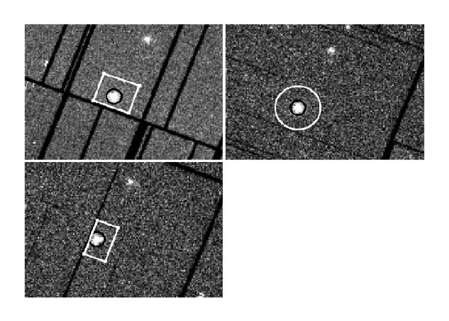
Figure 1: EPIC pn (upper left), MOS1 (upper right) and MOS2 (below) images of the Q2237+0305. Black circles define areas collecting source signal, while white-bordered areas show the regions chosen for estimates of the background.

2 Data reduction

GLS Q2237+0305 was observed with XMM-$\it{Newton}$ for an exposure time of 43.9 ks in 28 May 2002 (PI: Michael Watson; XMM-Newton public archive). Observation ID, date of observation, total source counts and count rates in the extraction regions can be found in Table 1.

dataset ID		0110960101
observation date		28.05.2002
	MOS	42.3
exposure time, (ks)	pn	39.6
	RGS	42.8
	MOS1	0.08
	MOS2	0.06
count rate, (count/s)	pn	0.29
	RGS1	0.11
	RGS2	0.10
	MOS1	3170
	MOS2	2542
total source counts	pn	11446
	RGS1	4707
	RGS2	4279

Table 1: XMM-Newton observation log for Q2237+0305. Here and throughout the paper the name “MOS” is used for the MOS1 and MOS2 together.

The European Photon Imaging Cameras (EPIC) MOS1, MOS2 and pn detectors were operated in full frame mode for the whole time of the observation. EPIC data and the data from the Reflection Grating Spectrometers (RGS) were processed with the XMM-$\it{Newton}$ Standard Analysis System (sas, public release version 6.5.0). After filtering of bad-flagged data, the effective exposure times were: 39.6 ks for pn-camera, 42.3 ks for MOS-cameras and 42.8 ks for RGS-spectrometers. The EPIC maps of Q2237+0305 are shown in Fig.1.

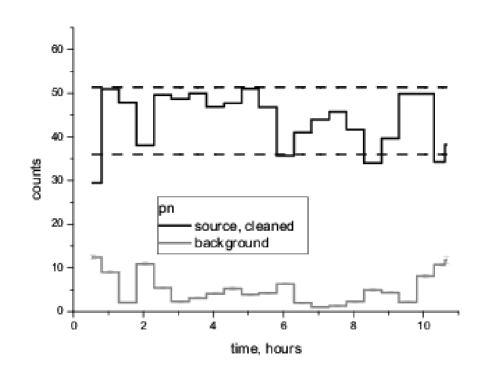
Figure 2: The full band (0.2-10 keV) EPIC pn lightcurves for the source (background-subtracted) and the background. The dashed straight lines show the $1\sigma$ limits of the averaged value of the flux during the observation time. The time bin size is 1.8 ks.

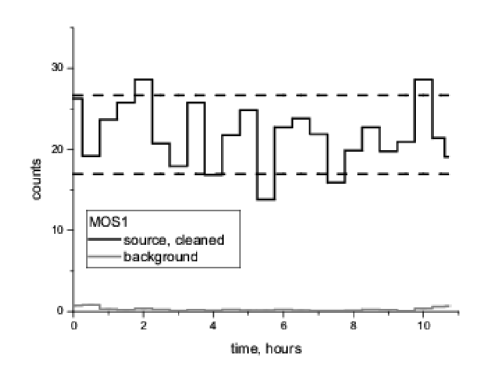
Figure 3: The same for EPIC MOS1 as in Fig. 2.

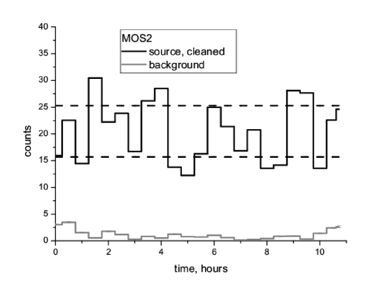
Figure 4: The same for EPIC MOS2 as in Fig. 2.

The energy range of EPIC cameras is 0.2–10 keV, and the RGS energy range is 0.3–2.8 keV. To obtain the cleaned lightcurves, we extracted full count rates from circular areas with different radii around the source (see Fig. 1). To estimate the background effects we also used areas of different sizes near the source on the same CCD plates. Flux variations from different background areas agree with the corresponding estimated Poisson variance. These variations have been taken into account in the final error estimates of the resulting net signal. The background counts were subtracted (with corresponding factors taking into account different background areas) from the total counts from the source regions to obtain the cleaned lightcurves. The best signal-to-background ratios at low enough levels of Poisson variance were obtained for the case of 3-5 arcsec radii of the source areas. The background-subtracted lightcurves are shown in Figs. 2 – 4 together with the corresponding background lightcurves.

EPIC spectra were obtained through standard sas procedures: evselect, arfgen, and rmfgen. For spectral filtering, the single high-energy events were extracted in order to identify soft proton flares ($E>10$ keV, for pattern zero only; the time-bin sizes were 100 s for the pn and 10 s for the MOS). Good time intervals were defined using the standard sas procedure tabgtigen (with rate parameter 1.0 cts/s for the pn camera and 0.35 cts/s for the MOS) and then the event files were corrected. The background subtracted EPIC spectra are shown in Fig. 5.

In the case of the lightcurves, we have not used tabgtigen, but we have simply subtracted the background counts from the total ones in order to obtain a continuous time series.

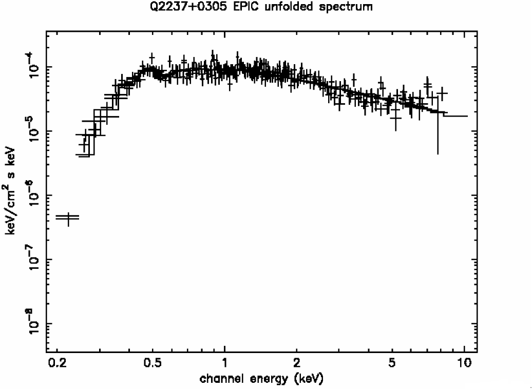
Figure 5: Unfolded XMM-Newton EPIC (pn and MOS) spectra of Q2237+0305 and power-law model. Here the 90% error bars are shown.

RGS spectra were obtained using standard sas tasks (rgsproc and rgsrmfgen). RGS lightcurves were obtained and background-subtracted similarly to the EPIC data (i.e., using an evselect procedure); they are characterized by larger errors than EPIC lightcurves. No significant absorption or emission lines were detected in these spectra.

3 Spectral fitting

To fit the Q2237+0305 spectrum, as a first step we tried a redshifted power-law model (zpowerlw)

$$\rho(E)=KE^{-\Gamma}$$

(where $\Gamma$ is the photon index), with photoelectric absorption (zphabs) by neutral material in the lensing galaxy

$$\rho(E)=Ke^{-\frac{\sigma(E)N_{H}}{1+z_{G}}}$$

where ${\sigma(E)}$ is the photo-electric cross-section and ${N_{H}}$ is hydrogen column density (see Table 2), using xspec v. 12.2.1. To calculate lensed luminosities, we used these values for the cosmological parameters: Hubble constant $H_{0}$=70 km/(s$\cdot$ Mpc), $\Lambda_{0}=0.7$ and $\Omega_{M}=0.3$. We compare fluxes and lensed luminosities in different rest-frame energy ranges obtained from our fit with spectral fits from Dai et al. (dai (2003)) and Wambsganss et al. (rosat (1999), see Table 3). The row labeled MOS in Table 2 refers to the MOS1 and MOS2 spectra fitted with the same model simultaneously, and the row labelled EPIC represents the MOS1, MOS2 and pn spectra fitted with the same model simultaneously. We obtained the values of $N_{H}$ for the lensing galaxy taking into account the mentioned above frozen value of the Galactic absorption (Dickey & Lockman, HI (1990)). The obtained values of photon indices and hydrogen column densities are in good agreement with the results of Dai et al. (dai (2003)), but our power-law indices are obviously higher than the power-law index of 1.5, assumed by Wambsganss et al. (rosat (1999)), likely due to the wider spectral range.

Camera	$N_{H}$,	$\Gamma$	$\chi^{2}$/d.o.f.	EW,
	$10^{20}$ cm-2			keV
MOS1	$9_{-4}^{+5}$	$1.86_{-0.16}^{+0.17}$	38.8/38	$<1.6$
MOS2	$8\pm$4	$1.94_{-0.11}^{+0.14}$	38.6/41	$<1.1$
pn	$5_{-2}^{+3}$	$1.85_{-0.12}^{+0.15}$	93.0/84	$<1.3$
MOS	$8\pm$3	$1.92\pm$0.10	80.1/83
EPIC	$7\pm$2	$1.88\pm$0.10	183.5/168

Table 2: Absorbed power-law fitting of XMM-$\it{Newton}$ Q2237+0305 spectra - hydrogen column density in the lens galaxy (at a redshift $z_{G}=0.0395$), photon index and $\chi^{2}$ / degrees of freedom (d.o.f). Estimated EW limits (right-most column, 90% confidence) are calculated for fixed values of $E=5.7$ keV and $\sigma=0.87$ keV. The name “MOS” is used for the MOS1 and MOS2 spectra modelled together; “EPIC” - for both MOS and pn spectra modelled together.

In Table 3 we report the XMM-$\it{Newton}$ fluxes and lensed luminosities together with the results from other authors, obtained from ROSAT and $\it{Chandra}$ observations. The fluxes obtained here are in good agreement with the $\it{Chandra}$ ones.

Satellite	Energy	$F,10^{-13}$	$L,$
Instr.	range, keV	erg/(cm${}^{2}\cdot$ s)	$10^{45}$ erg/s
XMM, MOS1	0.1-2.4	$2.5\pm$0.3
	0.4-8.0	$5.3_{-0.5}^{+0.4}$	11.8
	0.2-10.0	$6.0_{-0.7}^{+0.4}$	13.5
XMM, MOS2	0.1-2.4	$2.6_{-0.4}^{+0.3}$
	0.4-8.0	$5.4_{-0.6}^{+0.5}$	12.9
	0.2-10.0	$6.0_{-0.7}^{+0.3}$	14.6
XMM, pn	0.1-2.4	$2.4\pm$0.2
	0.4-8.0	$5.1_{-0.3}^{+0.4}$	10.4
	0.2-10.0	$5.8_{-0.5}^{+0.3}$	13.3
ROSAT	0.1-2.4	2.2	4.2
Chandra	0.4-8.0	$4.6_{-0.2}^{+0.4}$	10.0
	0.4-8.0	$3.7_{-0.5}^{+0.6}$	8.3

Table 3: Absorbed power-law fitting of XMM-$\it{Newton}$ Q2237+0305 spectra - fluxes and lensed luminosities.

Commonly considered as evidence of an accretion disk in the central engine of quasars or active galactic nuclei (AGN) is the detection of a broadened Fe K$\alpha$ emission line at a rest-frame energy of $\approx 6.4$ keV and a width in the range of 0.1–1.0 keV (see Laor, laor (1991)). Such lines were present in the spectra of 42% well-exposed objects from a sample of more than 100 AGN explored by Guainazzi et al. (guainazzi (2006)) and in the spectra of 2/3 of the 26 AGN from the sample analyzed by Nandra et al. (nandra (2007)). As shown by Reeves et al. (RPT (2004)) and Turner et al. (turner (2005)), a broadened Fe K$\alpha$ line can also be explained by the presence of an ionized absorber with a column density of $\approx 10^{23}$ cm^-2. However, Nandra et al. (nandra (2007)) show that 1/3 of the cases (in the considered sample) cannot be adequately fitted with an ionized gas model, and for all of them the line broadening mechanism is well explained by reflection from an accretion disk. In our case, the apparent lack in Q2237+0305 of prominent absorption (mentioned above) suggests that ionized absorber is likely not the case for this source. Taking into account the redshift of the quasar, the line should be observed between 2 and 3 keV. Dai et al. (dai (2003)) found the line at $5.7_{-0.3}^{+0.2}$ keV rest-frame energy, with $0.87_{-0.15}^{+0.30}$ keV line width and $1200_{-200}^{+300}$ eV equivalent width (EW), relying on the $\it{Chandra}$ (2000–2001) data.

In the case of the XMM-Newton observation of Q2237+0305, the Fe K$\alpha$ line is not evident. We try to model this line with the fixed rest-frame energy $E$ and line width $\sigma$ taken from Dai et al. (dai (2003)) to obtain an upper limit on its EW. The results are shown in Table 2. On the other hand, if we let the line energy and the width change over limited energy ranges (5–7 keV for the rest-frame energy and 0–1 keV for the line width), fitting of the pn spectrum yields $E=6.0_{-1.0}^{+0.7}$ keV rest-frame line energy and $\sigma<0.9$ keV for the line width; however, this result is not statistically significant (according to the $\chi^{2}$ test). For MOS1 and MOS2 such a treatment does not yield a meaningful result at all due to the lower counting statistics.

For completeness, we also fitted the pn spectrum of Q2237+0305 with a model often used for the spectral modelling of AGN (Soldi et al., soldi (2006), Schurch et al., schurch (2002)): a Compton-reflected (from neutral material) power-law energy distribution with high-energy cut-off $E_{c}$ (pexrav, Magdziarz & Zdziarski, Magd (1995)):

$$\rho(E)=KE^{-\Gamma}e^{-\frac{E}{E_{c}}}.$$

Neutral absorption in the lensing galaxy (zphabs) was also included here. The model with reflection provides a slightly better fit than a power-law ($\chi^{2}=1.05$ vs. $1.18$) which is, however, not statistically significant. Search for the high-energy cut-off ($E_{c}$) provided no results. The other parameters of this fit are as follows: photon index $\Gamma=2.3\pm$0.3, relative reflection parameter $R=2.3_{-1.2}^{+2.2}$, hydrogen column density in the lensing galaxy $N_{H}=7_{-2}^{+3}\cdot 10^{20}$ cm^-2 and flux of $F=6.0_{-2.0}^{+0.2}\cdot 10^{-13}$ erg/(cm${}^{2}\cdot$s) in the 0.2–10 keV energy range.

4 Lightcurves and variability

The photon counts $Y_{n}$ in every $n$-th time bin represent the total X-ray flux from all the images of GLS Q2237+0305 and have been obtained after background subtraction. The time bin size in this treatment was varied from $T=0.1$ to 2 ks.

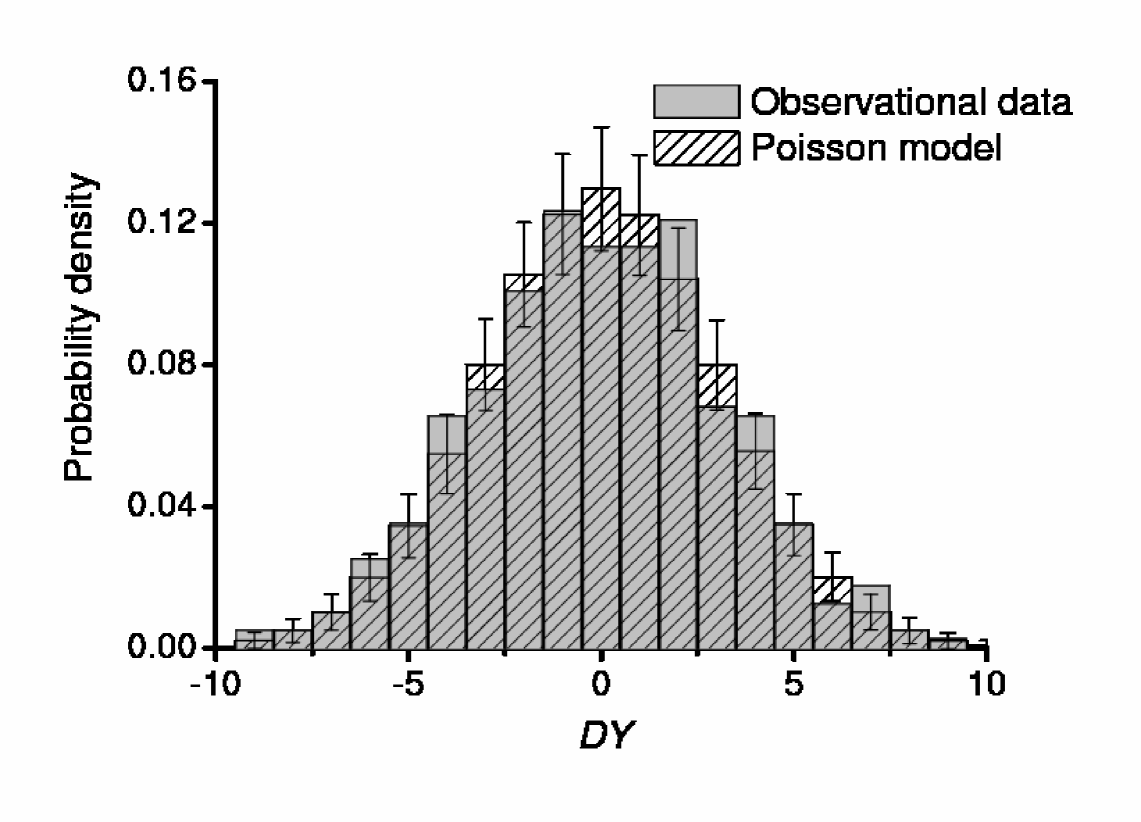
Figure 6: The distribution of the count differences $DY_{n}=Y_{n+1}-Y_{n}$, where $Y_{n}$ is the photon counts in every $n$-th bin. The observed distribution is shown with the shaded histogram and the expected distribution arising from Poisson noise is presented with the stripped histogram. The error bars are at the $1\sigma$ level.

Variability in $Y_{n}$ (estimated by the ratio of standard deviation $S$ to the mean $M$) is not noticeable in the lightcurves (Figs. 2, 3, 4). Numerical estimates are presented for 0.5 ks and 1 ks bin sizes (Table 4). Note that we do not observe a significant correlation (less than 0.2) between pn, MOS1, MOS2 data for various bin sizes which indicates that variations of the photon counts are simply due to their Poisson dispersion. We examined this question in more detail on the basis of the model of stationary Poisson process for the photon count numbers (i.e., with no variability). We considered the statistics of the observed count differences $DY_{n}=Y_{n+1}-Y_{n}$ and compared them to the statistics of simulated count differences in the case where the differences follow Poisson statistics. We find that the distribution $DY$ obtained from the observational data is very close to our simulated $DY$ distribution that assumes a Poisson model for the pn, MOS1 and MOS2 cameras. The distribution of $DY$ from the combined data of all the EPIC cameras is shown in Fig. 6. The $\chi^{2}$ test yields 91% probability that the distribution in Fig.6 is a realization of a Poisson process. Also we present in Fig.7 the structure function

$$F(n)=\frac{1}{N}\sum\limits_{i=1}^{N}{(Y_{i+n}-Y_{i})^{2}},$$

which agrees with Poisson model. Therefore, the hypothesis of constant X-ray flux from the source is compatible with the experimental data. The estimates reported above also apply for the 5–10 keV energy interval, with no substantial changes in variability.

Camera	$T,$	$V,$	$\nu$
	ks
pn	1	$\,0.13$	0.67
pn	0.5	0.24	0.89
MOS1	1	0.25	0.87
MOS1	0.5	0.40	0.99
MOS2	1	0.33	1.13
MOS2	0.5	0.40	0.96

Table 4: Parameters of the photon counts: $T$ is the time bin size. Variability is characterized by $V=S/M$, $S$ is the standard deviation and $M$ is the mean of $Y_{n}$; the parameter $\nu=S/\sqrt{M}$ compares $S$ with the calculated Poisson variance. The correlation of the net signal with the background in all the cases is less than $0.2$.

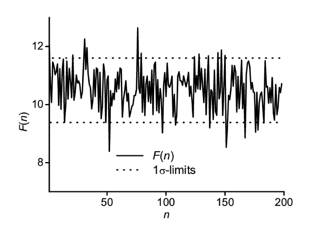
Figure 7: Structure function (total data from all EPIC cameras). Dashed straight lines show upper and lower $1\sigma$-limits estimated for a Poisson model. The time bin size is 100 s.

5 Discussion

We analysed the XMM-$\it{Newton}$ data (May, 2002) on the total X-ray flux from all four images of the GLS Q2237+0305 “Einstein Cross”. The flux value in the 0.2–10 keV range is $5.9\cdot 10^{-13}$ erg/(cm${}^{2}\cdot$ sec), corresponding to a lensed luminosity of $1.25\cdot 10^{46}$ erg/sec. In order to obtain the true quasar luminosity, this value must be corrected, taking into account the lens magnification. The most recent model estimate of the magnification is $16^{+5}_{-4}$ (Schmidt et al., schmidt (1998)). Fitting the X-ray spectra in the 0.2–10 keV energy range by an absorbed power-law yields the photon index $\Gamma=1.88\pm 0.10$ and hydrogen column density in the lensing galaxy $N_{H}=(7\pm$2)$\cdot 10^{20}$ cm^-2. This is in satisfactory agreement with the results of Dai et al. (dai (2003)).

The XMM-$\it{Newton}$ lightcurves obtained after the background subtraction are compatible with the hypothesis of a constant flux from the source. An additional argument in favor of no variability is the absence of a significant correlation between the light-curves from different cameras. This does not completely rule out source variability: (i) it may be obscured by the Poisson variance; (ii) it may be smeared out in the total X-ray flux from all the images that have different time delays; (iii) there may be periods of different variability amplitudes. These periods may correspond to the lifetimes of X-ray emitting blobs orbiting the black hole and therefore we might expect variability periods of the order of the revolution time around the black hole. In any case, the net variability during the XMM-$\it{Newton}$ observation cannot be large. As for concern (iii), we note that the ROSAT (1997) observations did not reveal significant variability. On the other hand, the variability was considerable during the $\it{Chandra}$ (2000, 2001) observations (Dai et al., dai (2003)). This suggests the presence of slow variability changes with characteristic times much longer than the inner variability timescale $\tau_{v}\sim 1$ hour following from the results of Dai et al. (dai (2003)).

Light-travel arguments imply that the one hour time-scale variability corresponds to a size-scale of the X-ray emitting region responsible for this variation of $R_{X}\sim\tau_{v}c/(1+z_{s})=4\cdot 10^{13}$ cm. An interesting question is whether $R_{X}$ represents an inhomogeneity in the accretion disk or the entire X-ray emitting region. This question might be answered, provided that the black hole mass in QSO 2237+0305 is known. Kochanek (kochan (2004)) estimated this mass, implying a radius of the innermost stable circular orbit of $3r_{g}\approx(4\div 22.5)\cdot 10^{14}$ cm (see, e.g., Chandrasekhar, chandrasekhar (1983)) in the case of a non-rotating black hole (where $r_{g}=2GM/c^{2}$ is the gravitational radius). The inner radius of a real accretion disk must be even larger. However, the mass estimate of Kochanek (kochan (2004)) is model dependent and it is not sufficient to make a rigorous judgement concerning a comparison with the order-of-magnitude estimate of $R_{X}$.

One may ask how this inhomogeneous structure (if it exists) would appear in the presence of microlensing. The theory of high-amplification events in the case of a small continuous source is well known (see, e.g., Grieger et al., grieger (1988); Shalyapin et al., shalyapin (2002); Popovic et al., popovic (2006) and references in these papers). In the case of one emitting spot, the microlensing amplification scales as $\sim R_{X}^{-1/2}$. Obviously, in the case of a large number of small inhomogeneities, the total amplification may be smeared out over the source. However, different regions of the time-dependent inhomogeneous structure will be differently amplified, resulting in an increase of the variability amplitude in microlensed image. Note that independent contributions of this microlensing effect may reduce the correlation between the lightcurves in different images. On the other hand, any prominent peak in the lightcurve without repetitions after the expected time delays can be considered as a probable sign of microlensing.

The idea of inhomogeneity of the quasar core in GLS has been repeatedly discussed from different viewpoints (see, e.g., Wyithe & Turner, wyither1 (2001); Wyithe & Loeb, wyither2 (2002); Schechter et al., schechter (2003)). Some evidence in favor of inhomogeneous structure may be found in optical observations of different GLSs, where the rapid flux variations are observed on the background of slower changes (Colley & Schild, colley (2003); Paraficz et al., paraficz (2006)). Note that there is an alternative explanation for these variations that invoke a planetary-mass object in the lensing galaxy (Schild & Vakulik, vakshild (2003), Colley & Schild, colley (2003)). It might be possible to distinguish between these two models by long-term optical and X-ray monitoring of microlensing events in AGN.

Observations of the resolved X-ray images with $\it{Chandra}$ are more informative for the Q2237+0305 variability studies and determination of the time delays. Nevertheless, observations of the total X-ray flux with XMM-$\it{Newton}$ may provide valuable complementary information on this issue. In the case of XMM-$\it{Newton}$, sufficiently long observations are needed to obtain a good result for the autocorrelation function. To avoid uncorrelated contributions from different images to the autocorrelation function, the monitoring period must be larger than the differential time delays in this system. In the case of Q2237+0305, the available measurement interval of almost 42 ks is clearly not long enough. The model prediction (Schmidt et al., schmidt (1998)) of maximal delay for Q2237+0305 is 17 hours. Large delays ($>35$ ks) are also predicted by earlier models of Q2237+0305 (Rix et al., rix (1992); Schneider et al., schneidtau (1988)). This is consistent with the analysis of the optical lightcurves of Q2237+0305 (Vakulik et al., vakulik (2006)), which yields an upper limit for the delays of about $\sim 2$ days.

While waiting for new observations one may ask whether in principle it is possible to determine the variable X-ray signal $x(t)$ from the source if the total flux from all the GLS images is available. Typically, this problem has an infinite number of solutions. However, if we know $x(t)$ over a sufficiently large initial interval, then $x(t)$ may be recovered uniquely from the total flux lightcurve (Zhdanov et al., zh (2003)). This may be of interest if one needs to combine results of long GLS monitoring of the total flux (cf. XMM-$\it{Newton}$) with shorter observations of separated different X-ray images (cf. $\it{Chandra}$).

- (1) Alcalde D., Mediavilla E., Moreau O. et al. 2002, in Aph. J. 572, 729.
- (2) Blanton M., Turner E., Wambsganss J. 1998, in MNRAS, 298, 1223.
- (3) Bliokh P.V., Dudinov V.N., Vakulik V.G. et al. 1999, in KFNT (Kiev, Ukraine), 15, 338.
- (4) Chandrasekhar S. 1983, The mathematical theory of black holes (Oxford-N.Y.).
- (5) Colley W.N., Schild R.E. 2003, in ApJ, 594, 97.
- (6) Dai X., Agol E., Bautz M.W., and Garmire G.P. 2003, in ApJ, 589, 100.
- (7) Dickey J.M., Lockman F.J. H I in the Galaxy. 1990, in A&A, 28, 215.
- (8) Falco E. E., Lehar J., Perley R. A., Wambsganss J., Gorenstein M.V. 1996, in AJ, 112, 897.
- (9) Grieger B., Kayser R., Refsdal S. 1988, in A&A, 194, 54.
- (10) Guainazzi M., Bianchi S., Dovciak M., 2006, in A&A, 88, 789.
- (11) Huchra J., Gorenstein M., Kent S. et al. 1985, in AJ, 90, 691.
- (12) Kochanek C.S. 2004, in ApJ, 605, 58.
- (13) Laor A. 1997, in ApJ, 376, 90.
- (14) Magdziarz P., Zdziarski A. A. 1995, in MNRAS, 273, 837.
- (15) Moreau O., Libbrecht C., Lee D.-W., Surdej J. 2005, in A&A, 436, 479.
- (16) Nadeau D., Racine R., Doyon R., Arboit G. 1999, in AJ, 527 (iss.1), 46.
- (17) Nandra K., O’Neill P.M., George I.M., Reeves J.N., 2007, in MNRAS, 382, 194.
- (18) Ostensen R., Refsdal S.,Stabell R. 1996, in A&A, 309, 59.
- (19) Paraficz D., Hjorth J., Burud I., Jakobsson P., Eliasdottir A. 2006, in A&A, 455, L1.
- (20) Popovic L. C., Jovanovic P., Petrovic T., Shalyapin V. N. 2006, in Astron.Nachr., 10, 981.
- (21) Reeves J. N., Porquet D., Turner T. J. 2004, in ApJ, 615, 150.
- (22) Rix H.-W., Schneider D.P., Bachcall J.N. 1992, in AJ, 104, 959.
- (23) Schild R., Vakulik V. 2003, in AJ, 126, 689.
- (24) Schechter P. L., Udalski A., Szymanski M., Kubiak M., Pietrzynski G. et al. 2003, in ApJ, 584, 657.
- (25) Schmidt R. W., Kundic T., Pen U. L. et al. 2002, in A&A, 392, 773.
- (26) Schmidt R., Webster R.L. & Lewis F.G. 1998, in MNRAS, 295, 488.
- (27) Schneider D.P., Turner E.L., Gunn J.E., et al. 1988, in AJ, 95, 1619.
- (28) Schneider P., Ehlers J., Falco E.E. 1992, Gravitational Lenses (Springer-Verlag).
- (29) Schurch N.J., Roberts T.P., Warwick R.S. 2002, in MNRAS, 335 (iss. 2), 241.
- (30) Shalyapin V.N., Goicoechea L.J., Alcalde D., Mediavilla E., Munoz J. A., Gil-Merino R. 2002, in AJ, 579, 127.
- (31) Soldi S., Beckmann V.S., Bassani L., Corvoizier T.J.-L. et al. 2005, in A& A, 444 (iss. 2), 431.
- (32) Spergel D.N.,Bean R., Dore O., Nolta M.R., Bennett C.L. et al. astro-ph/0603449.
- (33) Turner T. J., Kraemer S.B., George I.M., Reeves J.N., Bottorff M.C. 2005, in ApJ, 618, 155.
- (34) Vakulik V.G., Dudinov V.N., Zheleznyak A.P. et al. 1997, in Astron. Nachr., 318 (no.2), 73.
- (35) Vakulik V., Schild R., Dudinov V., Nuritdinov S., Tsvetkova V. et al. 2006, in A&A., 447, 905.
- (36) Wambsganss J., Brunner H., Schindler S., Falco E. 1999, in A&A, 346, L5.
- (37) Wambssganss J. & Pachinsky B. 1994, in AJ, 108, 1156.
- (38) Wozniak P., Alard C., Udalski A.et al. 2000, in AJ, 529, 88.
- (39) Wyithe, J.S.B., Loeb A. 2002, in ApJ, 577, 615.
- (40) Wyithe, J.S.B., Turner, E.L. 2001, in MNRAS, 320, 21.
- (41) Zhdanov V.I., Alexandrov A.N., Fedorova E.V. 2003, in Visnyk Kyivskogo Universitetu. Astronomy (Kiev, Ukraine), 39-40, 7.