Hyperentanglement witness

Abstract

A new criterium to detect the entanglement present in a hyperentangled state, based on the evaluation of an entanglement witness, is presented. We show how some witnesses recently introduced for graph states, measured by only two local settings, can be used in this case. We also define a new witness $W_{3}$ that improves the resistance to noise by increasing the number of local measurements.

I Introduction

Quantum entanglement represents the basic property underlying many quantum computation processes and quantum cryptographic schemes. It guarantees in principle secure cryptographic communications and a huge speedup of some important computation tasks. In this respect entanglement represents the basis of the exponential parallelism of the future quantum computers.

By using optical techniques the entanglement was realized in many experiments, either with quantum states based on two Kwiat et al. (1995), four Weinfurter and Żukowski (2001); Bourennane et al. (2004); Kiesel et al. (2005), or even six photons Lu et al. (2007), or, more recently, with multiphoton states, containing more than $10000$ entangled particles De Martini et al. (2008).

By hyperentanglement more degrees of freedom (DOF’s) of the photons are involved and entangled states spanning a high-dimension Hilbert space can be created Barbieri et al. (2005); Cinelli et al. (2005); Barreiro et al. (2005); Barbieri et al. (2004). A hyperentangled (HE) state encoded in $n$ DOF’s is expressed by the product of $n$ Bell states, one for each DOF. Double Bell HE states of two photons (i.e. with $n=2$) are currently realized in the laboratories and enable to perform tasks that are usually not achievable with normally entangled states. Among many applications, the realization of a complete Bell state analysis Barbieri et al. (2007); Schuck et al. (2006); Wei et al. (2007), and the recently realized enhanced dense codingBarreiro et al. (2008), are particularly worth of noting. By operating with HE states of two photons and $n$ independent DOF’s we are able to encode the information in $2n$ qubits. This significatively reduces the typical decoherence problems of multiphoton states based on the same number of qubits and dramatically increases the detection efficiency. HE states of increasing size are also important for the realization of advanced quantum nonlocality tests and represent a viable resource to increase the power of computation of a scalable quantum computer operating in the one-way model Briegel and Raussendorf (2001); Raussendorf and Briegel (2001). Indeed it has been recently demonstrated that efficient $4$-qubit $2$-photon cluster states are easily created starting from $2$-photon HE states Vallone et al. (2007); Chen et al. (2007); Vallone et al. (2008a, b).

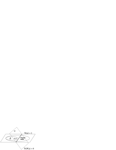
Figure 1: Geometrical representation of witnesses in the Hilbert space of hermitian operators $\rho$. In this space the scalar product is defined by $\langle\rho,\sigma\rangle\equiv\text{Tr}[\rho^{\dagger}\sigma]$. Physical states (i.e. the unit norm positive hermitian operators) lie on the hyperplane defined by $\langle\openone,\rho\rangle=\text{Tr}(\rho)=1$. The convex set $\mathcal{S}$ represents the separable states. We show also the completely mixed state $\openone/D\in\mathcal{S}$. The (hermitian) witness $W$ identifies a hyperplane (passing through the null state $\emptyset$) by the equation $\langle W,\rho\rangle\equiv\text{Tr}(W\rho)=0$ and splits the whole Hilbert space in two subsets, one of them containing $\mathcal{S}$. All the separable states $\sigma\in\mathcal{S}$ thus satisfy the condition $\langle\sigma,W\rangle\geq 0$ and lie on one side of the hyperplane. The physical states satisfying the condition $\langle\rho,W\rangle<0$ lie on the other side and thus are entangled.

The analysis of multiqubit entangled states performed by quantum state tomography is particularly demanding since the number of required measurements scales exponentially with the number of qubits. Furthermore, in practical realizations entanglement is degraded by decoherence and by any dissipation processes deriving from the unavoidable coupling with the environment. Being entanglement an expensive resource, its efficient detection with the minimum number of measurements is a crucial issue and new efficient analysis tools are necessary to characterize the entanglement of a particular multipartite state. The method of ”entanglement witness” Horodecki et al. (1996); Terhal (2000) (see Fig. 1 for a geometrical representation of an entanglement witness), first demonstrated for entangled states of two photons Barbieri et al. (2003) allows us to assess the presence of entanglement by using only a few local measurements. After its introduction the use of entanglement witness was extended to the detection of entanglement of various kinds of four qubit entangled states Bourennane et al. (2004); Kiesel et al. (2005); Walther et al. (2005); Vallone et al. (2007) and $N$-qubit cluster states. At the same time a big effort was spent in the study of the entanglement witness operator propertiesLewenstein et al. (2000, 2001); Bruß  et al. (2002); Gühne et al. (2002); Breuer (2006) and their non-linear generalizationGühne and Lütkenhaus (2006); Moroder et al. (2008).

By the present paper we address the timely question of finding a criterium to determine the presence of entanglement in HE states and introduce an entanglement witness which enables to detect entanglement in these states. This criterium is different from those used in case of multiparticle entangled states, where each qubits is encoded in a different particle. The difference resides in the different partitions that can be made in the two cases as it will be shown in the following section.

II Witness for hyperentangled state

Let’s consider the generic DOF $A_{j}$ ($B_{j}$), with $j=1,...n$, of particle $A$ ($B$). Each DOF spans a $2$-dimensional Hilbert space (i.e. it is equivalent to a qubit) whose basis is $\{{|0\rangle}_{A_{j}},{|1\rangle}_{A_{j}}\}$ ($\{{|0\rangle}_{B_{j}},{|1\rangle}_{B_{j}}\}$) for particle $A$ ($B$). In this way each particle encodes exactly $n$ qubits. Let’s define

$$\mathcal{U}\equiv\{A_{1},B_{1},\cdots,A_{n},B_{n}\}$$ (1)

the set containing the entire number of DOF’s. The (pure) HE state is written as

$$|\Xi\rangle={|\phi^{+}\rangle}_{A_{1}B_{1}}{|\phi^{+}\rangle}_{A_{2}B_{2}}\dots|\phi^{+}\rangle_{A_{n}B_{n}}\,,$$ (2)

where

$$|\phi^{+}\rangle_{A_{j}B_{j}}\equiv\frac{1}{\sqrt{2}}(|0\rangle_{A_{j}}|0\rangle_{B_{j}}+|1\rangle_{A_{j}}|1\rangle_{B_{j}})$$ (3)

represents a maximally entangled Bell state. In general $|\phi^{+}\rangle$ can be replaced with any maximally entangled state (this corresponds to apply single qubit unitaries on the HE state). In the language of graph states, a HE state can be interpreted as a graph state up to a Hadamard gate applied to each qubit $A_{j}$ (see Fig. 2).

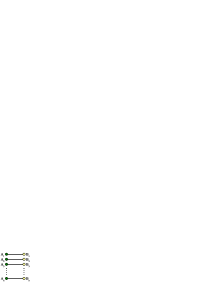
Figure 2: (Color online) A Hyperentagled state represented as a graph state where a dots corresponds to a qubit and the links represent the entanglement existing between the corresponding qubits. Dark (green) and bright (yellow) dots represent the degrees of freedom of particles $A$ and $B$ respectively.

Let’s define now the following $N=2n$ operators

$$\begin{cases}\begin{aligned} S_{2j}&=Z^{A}_{j}Z^{B}_{j}\\ S_{2j-1}&=X^{A}_{j}X^{B}_{j}\end{aligned}\qquad\qquad j=1,\cdots,n\end{cases}$$ (4)

where $Z^{A}_{j}$, $X^{A}_{j}$ ($Z^{B}_{j}$, $X^{B}_{j}$) are respectively the Pauli matrices $\sigma_{z}$ and $\sigma_{x}$ acting on the $j$th DOF of particle $A$ ($B$). By using the stabilizer formalism Gottesman (1996) the HE state can be also defined as the state satisfying

$$S_{k}|\Xi\rangle=|\Xi\rangle,\qquad\forall k=1,\cdots,N$$ (5)

In general we can define the stabilizer basis as

$$S_{k}|{\bf s}\rangle=(-1)^{s_{k}}|{\bf s}\rangle\,\quad\forall k=1,\cdots,N$$ (6)

$$|{\bf s}\rangle\equiv|[s_{1},s_{2},\cdots,s_{N}]\rangle\qquad s_{k}=0,1$$

and $|\Xi\rangle\equiv|[0,0,\cdots,0]\rangle$.

How can we detect entanglement in this case? And also: which kind of entanglement we would like to detect? The entanglement witness method is based on the introduction of a witness $W$, i.e. a hermitian operator whose expectation value is non negative for a generic separable state, while it is negative for the entangled state we want to detect. Since the witness is defined up to a multiplicative positive constant, here and in the following we fix the normalization of a generic witness $W$ for the HE state by requiring that

$$\langle\Xi|W|\Xi\rangle=-1$$ (7)

The advantages of this choice will become evident when the resistance to noise of the entanglement witness will be evaluated (see Section III).

Let’s define the entanglement we want to discriminate. A state $|\varphi\rangle$ is separable (in the hyperentangled sense) if it satisfies the following condition:

$$\exists j\text{ such that }|\varphi\rangle=|\varphi_{1}\rangle_{A_{j}\mathcal{I}}|\varphi_{2}\rangle_{B_{j}\mathcal{J}}$$ (8)

In this equation $\{\mathcal{I},\mathcal{J}\}$ represents a generic bi-partition of the set ${\mathcal{T}}_{j}\equiv\{A_{1},B_{1},\cdots,A_{n},B_{n}\}\backslash\{A_{j},B_{j}\}$, so that $\mathcal{I}\cup\mathcal{J}=\mathcal{T}_{j}$ and $\mathcal{I}\cap\mathcal{J}=\emptyset$.

Definition: A (mixed) state is defined to be hyperentangled in $n$ degrees of freedom if it is separately entangled in each of them and cannot be written as a mixture of states that satisfy (8).

In this way the possibility that a classical mixture of two or more states that are not entangled in each DOF, such as those satisfying eq. (8), can be interpreted as hyperentangled, is avoided. This definition of separability is different from the usual definition used in the multiparticle entanglement, where separability is referred to every possible partition of the qubits. In the hyperentanglement case a state is separable if it can be expressed by a partition that separates the same DOF, as written in equation (8). This condition is weaker then the usual multiparticle entanglement as it can be immediately seen by looking at the state $|\Xi\rangle$ in equation (2): this is a hyperentangled state if $A_{1},\cdots A_{n}$ ($B_{1},\cdots B_{n}$) refer the the different DOF’s of particle $A$ ($B$). However if any $A_{j}$ (or $B_{j}$) represents a different particle, the state $|\Xi\rangle$ is no more completely entangled (or “genuine multiparticle entangled”).

The first condition is the entanglement in every DOF. We can then measure $n$ entanglement witnesses. For each DOF $j$ we can introduce a witness given by:

$${\mathcal{W}^{(j)}=\openone_{2}-S_{2j}-S_{2j-1}.}$$ (9)

If all of them are negative,

$$\text{Tr}[\mathcal{W}^{(j)}\rho]<0\qquad\forall j=1,\cdots,n$$ (10)

we know that there is entanglement in each DOF. Hence all the reduced matrices

$$\rho_{j}=\text{Tr}_{\mathcal{U}\backslash{A_{j}B_{j}}}[|\Xi\rangle\langle\Xi|]\,,$$ (11)

obtained by tracing all the DOF’s but $A_{j}$ and $B_{j}$, are entangled.

In case of pure states the previous condition assures that each DOF of $A$ is entangled with the corresponding one of $B$. However this condition, although necessary, is not sufficient to demonstrate that the state cannot be created by a classical (i.e. mixed) superposition of states that are not entangled in all the DOFs. This is clearly explained by a simple example. Let’s consider the case with $n=2$ and two states

$$|\psi_{1}\rangle ={|0\rangle}_{A_{1}}{|0\rangle}_{B_{1}}{|\phi^{+}\rangle}_{A_{2}B_{2}}$$ (12)

$$|\psi_{2}\rangle ={|\phi^{+}\rangle}_{A_{1}B_{1}}{|0\rangle}_{A_{2}}{|0\rangle}_{B_{2}}$$

They are not entangled in every DOF since $|\psi_{1}\rangle$ ($|\psi_{2}\rangle$) is separable in the first (second) DOF. Then the two states are not hyperentangled:

$$\langle\psi_{1}|\mathcal{W}^{(2)}|\psi_{1}\rangle=\langle\psi_{2}|\mathcal{W}^{(1)}|\psi_{2}\rangle=-1\,,$$ (13)

$$\langle\psi_{1}|\mathcal{W}^{(1)}|\psi_{1}\rangle=\langle\psi_{2}|\mathcal{W}^{(2)}|\psi_{2}\rangle=0\,.$$

However by taking the mixture of these two states with equal weights, $\rho^{\prime}=\frac{1}{2}|\psi_{1}\rangle\langle\psi_{1}|+\frac{1}{2}|\psi_{2}\rangle\langle\psi_{2}|$, we obtain

$$\text{Tr}[\mathcal{W}^{(1)}\rho^{\prime}]=\text{Tr}[\mathcal{W}^{(2)}\rho^{\prime}]=-\frac{1}{2}$$ (14)

In this case the mixture of two non HE states is entangled in every DOF. Note that this feature doesn’t depend on the particular choice of the witness $\mathcal{W}^{(j)}$ in eq. (10).

The correct identification of a hyperentangled state can be obtained by introducing a hyperentanglement witness for the HE state $|\Xi\rangle$:

$$\widetilde{W} =\openone-2|\Xi\rangle\langle\Xi|$$ (15)

$$=\openone-\frac{2}{2^{N}}\sum_{\{s_{k}\}}S^{s_{1}}_{1}S^{s_{2}}_{2}\cdots S^{s_{N}}_{N}$$

In the Appendix we will show that

$$|\langle\Xi|\varphi\rangle|^{2}\leq\frac{1}{2}$$ (16)

for all the states $|\varphi\rangle$ that satisfy eq. (8). The expectation value of $\widetilde{W}$ is thus negative for $|\Xi\rangle$ but is positive for all the states expressed in the form (8), and then it is positive for all their mixtures. For example, it can be easily verified that for the state $\rho^{\prime}$ in (14) it holds $\text{Tr}[\widetilde{W}\rho^{\prime}]=0$ and hence $\rho^{\prime}$ is (correctly) not hyperentangled.

Given a witness $\widetilde{W}$, other witnesses $W^{\prime}$ can be derived on the basis of the following argument Tóth and Gühne (2005a, b): if we can find a constant $\alpha>0$ such that the operator $\mathcal{O}\equiv W^{\prime}-\alpha\widetilde{W}$ is positive definte (i.e. $\text{Tr}[\mathcal{O}\rho]\geq 0$, $\forall\rho$), then $W^{\prime}$ is a witness. In fact if $\text{Tr}[W^{\prime}\rho]<0$ on a generic state $\rho$ it comes out that $\text{Tr}[\widetilde{W}\rho]\leq\frac{1}{\alpha}\text{Tr}[W^{\prime}\rho]<0$ and thus $\rho$ is entangled.

Following this observation, it is shown in Tóth and Gühne (2005a, b) that the following operators

$$W_{1}=(N-1)-\sum^{N}_{k=1}S_{k}\,,\qquad\qquad$$ (17)

$$W_{2}=3-2\left(\prod_{\text{odd }k}\frac{S_{k}+1}{2}+\prod_{\text{even }k}\frac{S_{k}+1}{2}\right)$$ (18)

are witnesses for a generic connected graph state. The same argument can be repeated here, since it uses only the stabilizer equation. In fact, even in the case of a HE state (or whatever state defined in terms of the stabilized equation) the operators $W_{1}-\widetilde{W}$ and $W_{2}-\widetilde{W}$ are positive definte. This is simply checked in the stabilizer basis $|{\bf s}\rangle$ where they are diagonal and thier eigenvalues are non-negative.

We can also introduce here an other witness by using the same argument:

$$W_{3}=2-3\prod^{n}_{j=1}\left(\frac{1+S_{2j-1}+S_{2j}}{3}\right)$$ (19)

In order to demonstrate that $W_{3}$ is a witness, let’s consider $W^{\prime}_{3}=c_{0}-3\prod^{n}_{j=1}\left(\frac{1+S_{2j-1}+S_{2j}}{3}\right)$ and calculate the lowest eigenvalues of $\mathcal{O}_{3}\equiv W^{\prime}_{3}-\alpha\widetilde{W}$. If they are positives then $\mathcal{O}_{3}$ is positive definite. The lowest eigenvalues are $\lambda_{1}=c_{0}-\alpha-3+2\alpha$ for $|\Xi\rangle$ and $\lambda_{2}=c_{0}-\alpha-1$ for a state with only one $s_{k}$ equal to $1$. They are equal when $\alpha=1$ and are both positive when $c_{0}\geq 2$.

The witness (19) is built by considering all the possible products of stabilizers where, for each DOF, we can measure $\openone$, $XX$ or $ZZ$.

The four witnesses of above differ each other with respect to the number of measurement settings, i.e. their local decompositions Tóth and Gühne (2005b) are different. We remember that the local decomposition of $W$ is defined by the equation $W=\sum_{i}\mathcal{M}_{i}$, where $\mathcal{M}_{i}$ is measured by a different local measurement setting $\{O^{(k)}\}^{N}_{k=1}$. Each $\mathcal{M}_{i}$ then consists of the simultaneous measurements of $O^{(k)}$ on the corresponding qubit $k$.

In the case of $W_{1}$ and $W_{2}$ the local decomposition consists of two terms: the first is computed by the local setting $X_{1}X_{2}X_{3}X_{4}...$ and the second by $Z_{1}Z_{2}Z_{3}Z_{4}...$. Hence $W_{1}$ and $W_{2}$ require, as shown in Tóth and Gühne (2005b) only two local settings, while the number of settings needed for $\widetilde{W}$ and $W_{3}$ scales exponentially with $n$ (at most we need $3^{n}$ setting for $\widetilde{W}$ and $2^{n}$ measurement settings for $W_{3}$) Tóth and Gühne (2005a).

It is worth noting that the witness introduced in (9) can be measured by the same local settings needed for the measurements of $W_{1}$, $W_{2}$ (and of course by those used for $W_{3}$ and $\widetilde{W}$).

Moreover the advantage given by a low number of measurement settings for the witness $W_{1}$ and $W_{2}$ is paid by their weakness with respect to the resistance to noise. This will be shown in the following section.

III Resistance to noise

The strength of a witness if often measured by its resistance to noise, i.e. the amount of noise that can be added to the entangled state in such a way that the witness still measures it as entangled. Consider the following states

$$\rho=(1-p_{\text{noise}})|\Xi\rangle\langle\Xi|+p_{\text{noise}}\frac{1}{D}\openone$$ (20)

where we have defined $D=2^{N}$ and $p_{\text{noise}}$ measures the amount of (white) noise present in the state. The expectation value of a generic witness (normalized such that $\langle\Xi|W|\Xi\rangle=-1$) is given by

$$\text{Tr}[W\rho]=-1+p_{\text{noise}}+p_{\text{noise}}\frac{1}{D}\text{Tr}[W]$$ (21)

so the state is entangled if

$$\quad p_{\text{noise}}<\frac{D}{\text{Tr}[W]+D}\equiv p_{\text{M}}$$ (22)

where $p_{M}$ is the maximum allowed amount of noise. The trace of $W$ is thus a good measurement of the weakness of the witness: the lower the trace the stronger the resistance to noise. In table 1 we show the traces of the above defined witnesses in order of the increasing resistance to noise. While $\widetilde{W}$ is highly resistent to white noise ($p_{M}$ is always greater than $50\%$) but requires many measurement settings, $W_{1}$ and $W_{2}$ requires only two measurement settings but they are less resistent to noise. For any value of $N$ the resistance to noise of our defined witness (19) is larger than the witness $W_{2}$ and $W_{1}$, and $W_{3}$ can be seen as a compromise between the need of lowering the number of settings and that of increasing the noise resistance. In general (for any $N$) the noise tolerance of $W_{3}$ is at least $33\%$. In conclusion, the resistance to noise of the witness grows with the number of settings needed to evaluate it.

Witness	Tr[$W$]	$p_{M}$
$W_{1}$	$(N-1)D$	$\frac{1}{N}=\frac{1}{\log_{2}D}\geq 0$
$W_{2}$(even $N$)	$3D-4\sqrt{D}$	$\frac{1}{4}\frac{1}{1-\frac{1}{\sqrt{D}}}\geq\frac{1}{4}$
$W_{2}$(odd $N$)	$3D-3\sqrt{2D}$	$\frac{1}{4}\frac{1}{1-\frac{3}{4\sqrt{2D}}}\geq\frac{1}{4}$
$W_{3}$(even $N$)	$2D-\frac{3D}{(\sqrt{D})^{\log_{2}3}}$	$\frac{1}{3}\frac{1}{1-\frac{1}{(\sqrt{D})^{\log_{2}3}}}\geq\frac{1}{3}$
$W_{3}$(odd $N$)	$2D-\frac{3D}{2(\sqrt{D/2})^{\log_{2}3}}$	$\frac{1}{3}\frac{1}{1-\frac{1}{2(\sqrt{D/2})^{\log_{2}3}}}\geq\frac{1}{3}$
$\widetilde{W}$	$D-2$	$\frac{1}{2}\frac{1}{1-\frac{1}{D}}\geq\frac{1}{2}$

Table 1: Traces of the witness operator defined in the text and their corresponding resistance to the white noise. The number $p_{M}$, depending on the dimension $D$ of the Hilbert space, represents the maximum amount of noise tolerated by the corresponding hyperentanglement witness.

IV New entanglement witness for generic graph states

The same witness defined in (19) can be used for a generic graph state $|G_{N}\rangle$ associated to a connected graph of $N$ vertices. The graph state is defined by the stabilizer equation as

$$S_{k}|G_{N}\rangle=|G_{N}\rangle,\qquad\forall k=1,\cdots,N$$ (23)

where

$$S_{k}=X_{k}\prod_{j\in\mathcal{N}_{k}}Z_{j}\qquad\quad k=1,\cdots,N\\$$ (24)

Here $X_{k}$ ($Z_{k}$) are the Pauli matrix $\sigma_{x}$ ($\sigma_{z}$) acting on qubit $k$ and $\mathcal{N}_{k}$ is the set of qubits to which it is linked. As shown in Bourennane et al. (2004), for a given connected graph, the following witness detects the genuine N-qubit entanglement of the corresponding graph state $|G_{N}\rangle$:

$$\widetilde{W}=\openone-2|C_{N}\rangle\langle C_{N}|$$ (25)

Each state of the form $|\phi_{1}\rangle_{\mathcal{A}}|\phi_{2}\rangle_{\mathcal{B}}$ (where $\mathcal{A},\mathcal{B}$ is a generic partition of the $N$ qubits) has a positive expectation value of this witness.

Following the same arguments of the previous section it is possible to show that the followign operator is a witness

$$W_{3}=\begin{cases}2-3{\displaystyle\prod^{n}_{j=1}}\left(\frac{1+S_{2j-1}+S_{2j}}{3}\right)\qquad N=2n\\ 2-3{\displaystyle\prod^{n}_{j=1}}\left(\frac{1+S_{2j-1}+S_{2j}}{3}\right)\frac{1+S_{N}}{2}\qquad N=2n+1\end{cases}$$ (26)

The number of settings needed for $\widetilde{W}$ scales exponentially with the number of qubits Tóth and Gühne (2005a), while we need more than two measurement settings to determine $W_{3}$. The maximum amount of noise $p_{M}$ allowed for $W_{3}$ is shown in table 1.

V conclusions

In this paper we have introduced a method to detect if a 2-particle state is hyperentangled. The method is based on the initial detection of entanglement for each separate degree of freedom. Once this condition is satisfied the negative value of a hyperentanglement witness operator detects the hyperentanglement. We introduced four different hyperentanglement witnesses, namely $\widetilde{W}$, $W_{1}$, $W_{2}$ and $W_{3}$. They are characterized by different values of the resistance to noise which grows with the number of measurement settings needed for their evaluation. Precisely, only two local settings are required in the case of $W_{1}$ and $W_{2}$, while for $W_{3}$ and $\widetilde{W}$ their number scales exponentially with the number of DOFs. It is worth noting that the local setting used to measure $\widetilde{W}$, $W_{1}$, $W_{2}$ and $W_{3}$ can be also used to measure the witnesses $\mathcal{W}^{(j)}$ (see equation (9)) and then reveal the entanglement corresponding to each DOF, separately. For example with the local setting $Z_{1}Z_{2}Z_{3}Z_{4}Z_{5}Z_{6}\dots$ it is possible to measure the observables $S_{2}$, $S_{4}$, $S_{6}$, $\dots$ and all their products.

A low number of measurements corresponds to a reduced resistance to noise. Indeed, it is shown that the amount of white noise tolerated by $W_{3}$ and $\widetilde{W}$ exceeds those tolerated by $W_{1}$ and $W_{2}$ (see table (1)).

In general, a hyperentangled state (2) can also be expressed as a maximally entangled state of two qu$d$it, where $d=2^{n}$, since each particle encodes $n$ qubits. However our approach is different from the usual bipartite qudit entanglement since the witness detecting the bipartite entanglement between the two particles is (up to normalization) $W=\frac{\openone}{2^{n}}-|\Xi\rangle\langle\Xi|$ since the maximum overlapp between a maximally entangled state of two qu$d$it and a separable state is exactly $\frac{1}{2^{n}}$. The witness (15) is far more stringent since many entangled states in the bipartite sense are not hyperentangled. For example the state $|\psi_{1}\rangle$ in (12) can be written as $|00\rangle_{A}|00\rangle_{B}+|01\rangle_{A}|01\rangle_{B}$. This state clearly shows entanglement between $A$ and $B$ but it is not hyperentangled.

Appendix A Demonstration

Let the state $|\varphi\rangle$ satisfy eq. (8). This means that $j$ must exist such that $|\varphi\rangle$ can be written as

$$|\varphi\rangle= |\varphi_{1}\rangle_{A_{j}\mathcal{I}}|\varphi_{2}\rangle_{B_{j}\mathcal{J}}$$ (27)

$$= (a|0\rangle_{A_{j}}|\chi_{1}\rangle_{\mathcal{I}}+b|1\rangle_{A_{j}}|\chi_{2}\rangle_{\mathcal{I}})$$

$$\otimes(c|0\rangle_{B_{j}}|\chi_{3}\rangle_{\mathcal{J}}+d|1\rangle_{B_{j}}|\chi_{4}\rangle_{\mathcal{J}})$$

with $|\chi_{i}\rangle$ normalized and $|a|^{2}+|b|^{2}=|c|^{2}+|d|^{2}=1$. Let’s define $\gamma_{\mu\nu}$ the overlapp between $|\chi_{\mu}\rangle_{\mathcal{I}}|\chi_{\nu}\rangle_{\mathcal{J}}$ and ${\langle\phi^{+}|}_{A_{1}B_{1}}\dots\langle\phi^{+}|_{A_{j-1}B_{j-1}}{\langle\phi^{+}|}_{A_{j+1}B_{j+1}}\dots\langle\phi^{+}|_{A_{n}B_{n}}$. Since the states $|\chi_{i}\rangle$ are normalized we have $|\gamma_{\mu\nu}|^{2}\leq 1$. By calculating the overlapp we obtain

$$|\langle\Xi|\varphi\rangle|^{2} =\langle\phi^{+}|\left(ac\gamma_{13}|00\rangle+ad\gamma_{14}|01\rangle+bc\gamma_{23}|10\rangle+bd\gamma_{24}|11\rangle\right)_{A_{j}B_{j}}=\frac{1}{2}|(ac\gamma_{13}+bd\gamma_{24})|^{2}$$ (28)

$$\leq\frac{1}{2}\left(|(ac\gamma_{13}|^{2}+|bd\gamma_{24}|^{2}\right)\leq\frac{1}{2}\left(|ac|^{2}+|bd|^{2}\right)\leq\frac{1}{2}\left(|a|^{2}+|b|^{2}\right)=\frac{1}{2}$$

where we used $|\gamma_{\mu\nu}|^{2},|c|^{2},|d|^{2}\leq 1$ and the property $|r+s|^{2}\leq|r|^{2}+|s|^{2}$. The bound is easily saturated, for example by the states of the form

$${|\phi^{+}\rangle}_{A_{1}B_{1}}\dots|\phi^{+}\rangle_{A_{j-1}B_{j-1}}{|0\rangle}_{A_{j}}{|0\rangle}_{B_{j}}{|\phi^{+}\rangle}_{A_{j+1}B_{j+1}}\dots|\phi^{+}\rangle_{A_{n}B_{n}}.$$ (29)

References

- Kwiat et al. (1995) P. G. Kwiat, K. Mattle, H. Weinfurter, A. Zeilinger, A. V. Sergienko, and Y. Shih, Phys. Rev. Lett. 75, 4337 (1995).
- Weinfurter and Żukowski (2001) H. Weinfurter and M. Żukowski, Phys. Rev. A 64, 010102 (2001).
- Bourennane et al. (2004) M. Bourennane, M. Eibl, C. Kurtsiefer, S. Gaertner, H. Weinfurter, O. Gühne, P. Hyllus, D. Bruß , M. Lewenstein, and A. Sanpera, Phys. Rev. Lett. 92, 087902 (2004).
- Kiesel et al. (2005) N. Kiesel, C. Schmid, U. Weber, G. Tóth, O. Gühne, R. Ursin, and H. Weinfurter, Phys. Rev. Lett. 95, 210502 (2005).
- Lu et al. (2007) C.-Y. Lu, X.-Q. Zhou, O. Gühne, W.-B. Gao, J. Zhang, Z.-S. Yuan, A. Goebel, T. Yang, and J.-W. Pan, Nature Phys. 3, 91 (2007).
- De Martini et al. (2008) F. De Martini, F. Sciarrino, and C. Vitelli, Phys. Rev. Lett. 100, 253601 (pages 4) (2008).
- Barbieri et al. (2005) M. Barbieri, C. Cinelli, P. Mataloni, and F. De Martini, Phys. Rev. A 72, 052110 (2005).
- Cinelli et al. (2005) C. Cinelli, M. Barbieri, F. De Martini, and P. Mataloni, Las. Phys. 15, 124 (2005).
- Barreiro et al. (2005) J. T. Barreiro, N. K. Langford, N. A. Peters, and P. G. Kwiat, Phys. Rev. Lett. 95, 260501 (2005).
- Barbieri et al. (2004) M. Barbieri, C. Cinelli, F. De Martini, and P. Mataloni, Fortschr. Phys. 52, 1102 (2004).
- Barbieri et al. (2007) M. Barbieri, G. Vallone, P. Mataloni, and F. De Martini, Phys. Rev. A 75, 042317 (2007).
- Schuck et al. (2006) C. Schuck, G. Huber, C. Kurtsiefer, and H. Weinfurter, Phys. Rev. Lett. 96, 190501 (2006).
- Wei et al. (2007) T.-C. Wei, J. T. Barreiro, and P. G. Kwiat, Phys. Rev. A 75, 060305(R) (2007).
- Barreiro et al. (2008) J. T. Barreiro, T.-C. Wei, and P. G. Kwiat, Nature Physics 4, 282 (2008).
- Briegel and Raussendorf (2001) H. J. Briegel and R. Raussendorf, Phys. Rev. Lett. 86, 910 (2001).
- Raussendorf and Briegel (2001) R. Raussendorf and H. J. Briegel, Phys. Rev. Lett. 86, 5188 (2001).
- Vallone et al. (2007) G. Vallone, E. Pomarico, P. Mataloni, F. De Martini, and V. Berardi, Phys. Rev. Lett. 98, 180502 (2007).
- Chen et al. (2007) K. Chen, C.-M. Li, Q. Zhang, Y.-A. Chen, A. Goebel, S. Chen, A. Mair, and J.-W. Pan, Phys. Rev. Lett. 99, 120503 (2007).
- Vallone et al. (2008a) G. Vallone, E. Pomarico, F. De Martini, and P. Mataloni, Phys. Rev. Lett. 100, 160502 (2008a).
- Vallone et al. (2008b) G. Vallone, E. Pomarico, F. De Martini, and P. Mataloni, Las. Phys. Lett. 5, 398 (2008b).
- Horodecki et al. (1996) M. Horodecki, P. Horodecki, and R. Horodecki, Phys. Lett. A 223, 1 (1996).
- Terhal (2000) B. M. Terhal, Phys. Lett. A 271, 319 (2000).
- Barbieri et al. (2003) M. Barbieri, F. De Martini, G. Di Nepi, P. Mataloni, G. M. D’Ariano, and C. Macchiavello, Phys. Rev. Lett. 91, 227901 (2003).
- Walther et al. (2005) P. Walther, K. J. Resch, T. Rudolph, E. Schenck, H. Weinfurter, V. Vedral, M. Aspelmeyer, and A. Zeilinger, Nature 434, 169 (2005).
- Lewenstein et al. (2000) M. Lewenstein, B. Kraus, J. I. Cirac, and P. Horodecki, Phys. Rev. A 62, 052310 (2000).
- Lewenstein et al. (2001) M. Lewenstein, B. Kraus, P. Horodecki, and J. I. Cirac, Phys. Rev. A 63, 044304 (2001).
- Bruß et al. (2002) D. Bruß , J. I. Cirac, P. Horodecki, F. Hulpke, B. Kraus, M. Lewenstein, and A. Sanpera, J. Mod. Opt. 49, 1399 (2002), eprint [quant-ph/0110081].
- Gühne et al. (2002) O. Gühne, P. Hyllus, D. Bruß, A. Ekert, M. Lewenstein, C. Macchiavello, and A. Sanpera, Phys. Rev. A 66, 062305 (2002).
- Breuer (2006) H.-P. Breuer, Phys. Rev. Lett. 97, 080501 (2006).
- Gühne and Lütkenhaus (2006) O. Gühne and N. Lütkenhaus, Phys. Rev. Lett. 96, 170502 (2006).
- Moroder et al. (2008) T. Moroder, O. Gühne, and N. Lütkenhaus (2008), preprint, eprint [arXiv:0806.0855].
- Gottesman (1996) D. Gottesman, Phys. Rev. A 54, 1862 (1996).
- Tóth and Gühne (2005a) G. Tóth and O. Gühne, Phys. Rev. Lett. 94, 060501 (2005a).
- Tóth and Gühne (2005b) G. Tóth and O. Gühne, Phys. Rev. A. 72, 022340 (2005b).