Informed Network Coding for Minimum Decoding Delay

Abstract

Network coding is a highly efficient data dissemination mechanism for wireless networks. Since network coded information can only be recovered after delivering a sufficient number of coded packets, the resulting decoding delay can become problematic for delay-sensitive applications such as real-time media streaming. Motivated by this observation, we consider several algorithms that minimize the decoding delay and analyze their performance by means of simulation. The algorithms differ both in the required information about the state of the neighbors’ buffers and in the way this knowledge is used to decide which packets to combine through coding operations. Our results show that a greedy algorithm, whose encodings maximize the number of nodes at which a coded packet is immediately decodable significantly outperforms existing network coding protocols.

I Introduction

The basic idea of network coding [1, 2], by which nodes transmit packets that result from joint encoding of multiple original information units, has led to communication protocols that are applicable in a wide range of wireless communication scenarios [3]. The gains brought by network coding are most evident in applications involving multicast or broadcast sessions (in which messages are intended for multiple destination nodes) in combination with physical layer broadcast (in which neighboring nodes can overhear potentially useful information).

For delay-sensitive applications such as media streaming, it is not desirable for receivers to have to wait for the arrival of several packets until they are able to decode the sent data. Instead, we would like for a packet to be immediately decodable given only the information units already available at those nodes. Moreover, each packet should be useful for as many neighbors as possible, thus minimizing the required number of transmissions. Similar considerations hold for distributed systems with highly constrained nodes, such as sensor networks, where it may well be impossible to store a large number of coded packets and to decode them using Gaussian elimination.

In general, there is a tradeoff between delay, throughput and end-to-end quality, and different codes can try to optimize either one of these performance metrics. Priority Encoded Transmission [4] provides graceful degradation by specifying different levels of coding (and consequently different minimum numbers of packets required for decoding) depending on the content and the priority of the underlying information units. Fountain codes (e.g. Raptor codes [5]) offer very low coding overhead and are (asymptotically) rate optimal when transmitting over erasure channels. However, decoding $n$ packets is only possible after $n+\epsilon$ coded packets have been received. A fraction of the encoded symbols can be decoded earlier albeit at the cost of significant overhead [6].

We focus our attention on algorithms that allow immediate decoding of each incoming packet. This stringent delay requirement comes at the cost of a reduction in throughput in the sense that broadcasting coded packets brings new information to fewer neighbors than fountain coding or priority encoded transmission would allow. Fostering early or immediate decoding requires an algorithm that decides which and how many information units or symbols should be combined in each new packet that is to be transmitted.

Adequate design of such an algorithm is highly dependent on the state information available at the nodes. Complete lack of state information is likely to occur in highly dynamic networks, such as mobile sensor networks, where the overhead of tracking a changing neighborhood would be prohibitive. In case a node has no information about the packets that have already been recovered by its neighbors, the algorithm can only optimize how many information units to combine (i.e., the codeword degree [7]). Each node simply combines randomly chosen information received from other nodes with its own information units, until the desired codeword degree is reached. The algorithm needs to find the right tradeoff between a high codeword degree that ensures that coded packets bring new information to many of the neighbors, and a low codeword degree that allows packets to be decoded immediately using only the information that is locally available. An analysis of optimum degree distributions with respect to network dynamics and topology was carried out in [8].

When information about the data recovery status of neighboring nodes is available, it is possible to employ more sophisticated coding algorithms. One such instance is presented in [9], which proposes a protocol for unicast routing in wireless mesh networks. Routers combine packets opportunistically from different sources in order to increase the diversity of the information content of each transmission. A node chooses the symbols to combine based on the content of the neighbors’ buffers. This form of state information is piggybacked onto data packets and also extrapolated from past loss rate measurements and overheard packets. The procedure ensures that coded packets are immediately decodable at the next hop with very high probability.

Although the protocol in [9] targets unicast traffic, very similar considerations also apply to broadcast. [10] analyzes a number of simple heuristics for the online and offline version of the problem.

Intrigued by the behavior of network coding protocols for one-to-all or all-to-all information dissemination, we compare the performance of several existing coding algorithms with various levels of buffer state information on neighboring nodes. We further propose two new protocols, one that maximizes the number of immediately decodable packets in a greedy fashion, and one that attempts to equalize the number of recovered information units among neighbors. The proposed schemes operate under the assumption that neighboring nodes exchange information about which symbols they have already recovered, for example by appending this information every time they send a data packet.

We show that the proposed schemes outperform existing algorithms in various scenarios of interest. We first consider a simple decoder that discards all incoming packets that cannot be decoded immediately. We then proceed with a characterization of the performance gains induced by a more complex decoder that buffers all received packets and uses Gauss-Jordan elimination to recover the sent data.

The remainder of the paper is structured as follows. In Section II we discuss related coding algorithms that shall serve as a baseline for the subsequent comparison. Section III describes our two network coding algorithms, whose performance is highlighted in Section IV, where simulation results are used to compare their performance to that of existing solutions. Section V concludes the paper.

II Review of Existing Coding Algorithms

Network coding enables nodes to transmit packets that are a combination of multiple original data packets. For this purpose, coding operations are applied to symbols (or sequences of bits), which can be viewed as elements of a finite field. When combining a set of packets, the same operations are applied to all of the symbols that form these packets and consequently the output packet has the same length as the input packets. Linear codes have been shown to be sufficient to achieve the multicast capacity of a network and can be easily implemented in practice.

Network coding schemes often generate each coded packet in a randomized fashion by taking into consideration all the packets that are available in the send buffer. This approach requires no knowledge about the recovery status of the neighboring nodes and no pre-established degree distribution (as explained later). The most prominent representative of this class of schemes is the Random Linear Network Coding (RLNC) algorithm presented in [11], where the coefficients used to generate the output linear combination are chosen randomly from the prescribed field.

The algorithms presented in the next section are based on the simplest form of network coding, whose single operation is binary addition (in contrast with RLNC, which generally requires addition and multiplication in higher fields). Since the symbols are elements of the binary field, adding two packets amounts to the bit-wise XOR of their symbols. It is worth mentioning, however, that the design considerations presented in this paper also hold for fields of larger size.

Regarding the decoding process, we consider two different mechanisms: (1) a very simple decoding scheme, which uses only immediately recovered symbols for decoding a new symbol from a received packet; and (2) the full decoding scheme, which performs Gaussian-Jordan elimination based on both coded and undecoded packets that are stored in a node’s buffer.

As an example of a RLNC scheme, we now give a formal definition of the algorithm presented in [10]. This Systematic Random Network Coding scheme was designed for the scenario of a source broadcasting to $n$ receivers over independent erasure channels.

Systematic Random Network Coding [10]: The algorithm starts by sending every packet once in uncoded form. After this first phase, the algorithm computes the output packet as a random linear combination of all the (uncoded) packets in the buffer.

Since the systematic algorithm produces random linear combinations of all the packets in the send buffer, the original symbols can only be recovered by means of Gauss-Jordan Elimination and only after enough independent linear combinations have been gathered by the destination node. In general, these coded symbols cannot be recovered at an earlier stage thus defeating a simple decoder, which discards all packets that are not immediately decodable using solely the already decoded information. It is therefore necessary to limit the number of symbols combined at each step, also called the codeword degree.

II-A Degree distribution based algorithm

Network coding schemes that combine all packets in the buffer are not always optimal in terms of performance, as observed in [7]. The authors show that depending on the number of recovered packets $r$ at a specific node, there exists an optimal number of packets to combine to maximize the number of decodable packets at each instant in time. More precisely, defining the codeword degree as the number of original symbols which are jointly encoded to form a coded packet, the authors of [7] determine the optimum degree distribution. For a prescribed number of recovered packets $r$, the degree distribution $D(r)$ returns the degree of the next output packet.

The scenario studied in [7] is a random encounter scenario, in which each node meets independently at random one neighbor at a time. The optimum degree distribution depends on the dynamics of the underlying network and in [12] the authors show the deficiencies of such an algorithm in scenarios beyond the specific model they were designed for. Since [7], some other coding algorithms based on a pre-defined degree distribution were proposed. As a comparison algorithm, we use the following instance.

Adaptive Network Coding (ANC) [8]: When a transmission opportunity occurs, the node randomly combines a specific number of packets in its buffer, which ensures that the degree of the resulting output packet is as high as possible and less than or equal to $D(r)$ (as defined above).

II-B Opportunistic Algorithm

The previous algorithms do not make use of feedback information in terms of the recovery state of neighboring nodes. However, if available, this additional information can be be used to make more efficient coding decisions and can bring significant improvements to the overall performance. The work presented in [10] analyzes how it can be used and proposes a number of heuristic algorithms designed for the scenario of a source node broadcasting to $n$ receivers over independent erasure channels, i.e. a one-to-all broadcast scenario. Among the algorithms proposed in [10], we consider the so called Opportunistic algorithm, because it is the only one that can be used in conjunction with a simple decoder. The basic idea is that each node uses the feedback received from its neighbors to compute a queue of symbols that have not yet been received by at least one node. The first symbol is chosen randomly and further symbols are added under the condition that the packet remains immediately decodable by all neighbors that were previously able to decode it (in other words, the number of nodes that can decode the packet can only increase).

Before defining a different set of algorithms capable of exploiting the knowledge of the recovery status of neighboring nodes, we must introduce some basic notation. In the following, we will denote the node performing the coding algorithm by $x$. The set of neighbors of node $x$ is denoted by $N_{x}=\{1,\dots,m\}$ and $B_{x}=\{s_{1},\dots,s_{n}\}$ denotes the set of symbols in the buffer of node $x$. $B_{j}$ represents the set of symbols that are in the buffer of node $j$, with $j\in N_{x}$. The set of symbols that are in the buffer of $x$ and that are not in the buffer of neighbor $j$ is denoted by $\overline{B}_{j}$ and can be computed as $\overline{B}_{j}=B_{x}\backslash(B_{j}\cap B_{x})$.

The algorithms presented next start by choosing the set of symbols $C$ that will be combined in the output packet by means of an XOR operation. The set $C$ is constructed iteratively, such that in each step of the algorithm one symbol is added to the previously constructed set. $\overline{C}$ denotes the set of symbols that node $x$ has in its buffer and that are not in $C$ (it can be calculated as $\overline{C}=B_{x}\backslash C$).

Finally, we will denote by $R(C)$ the set of neighbors of node $x$ that are able to recover a new symbol from the XOR of all symbols in a given set $C$. This means that, if there are $y$ symbols in set $C$, the neighbor must have already recovered exactly $y-1$ of the symbols in $C$. Therefore, we have that $R(C)=\{j:|C|-|B_{j}\cap C|=1\}$.

We are now ready to give a formal definition of the Opportunistic scheme, presented in [10].

Algorithm 1 Opportunistic algorithm [10]

$\ \ \ \ \ \ \ \ C=\emptyset$
$\ \ \ \ \ \ \ \ S=\{s\in B_{x}:|R(\{s\})|>0\}$
$\ \ \ \ \ \ \ \ \textrm{while }|S|>0$
$\ \ \ \ \ \ \ \ \ \ \ \ \ \ \ \ \textrm{choose }s^{*}\in S$
$\ \ \ \ \ \ \ \ \ \ \ \ \ \ \ \ \textrm{add }s^{*}\textrm{ to }C$
$\ \ \ \ \ \ \ \ \ \ \ \ \ \ \ \ S=\left(\bigcap\limits_{j\in R(C)}(B_{j}\cap B_{x})\right)\cap\overline{C}$
                end
$\ \ \ \ \ \ \ \ p=\bigoplus\limits_{s\in C}s$
                transmit $p$.

As shown in Algorithm 1, the set $C$ is initialized to the empty set. Throughout the algorithm, set $S$ represents the set of symbols that can be added to the current configuration of set $C$. Initially, all the symbols that are in the buffer of node $x$ and that are not in the buffer of at least one neighbor are deemed to be possible candidates. Thus, because $R(\{s\})$ is the set of neighbors that has not recovered symbol $s\in B_{x}$, $S$ is initialized according to $S=\{s\in B_{x}:|R(\{s\})|>0\}$.

Next, we focus on the loop in the algorithm, which will only continue while $S$ is non-empty. As long as there are symbols in $S$, the algorithm chooses one of them randomly and adds it to $C$. After this step, it is necessary to update $S$, from which the algorithm chooses new symbols to add to $C$.

The new set $S$ is defined as the set of symbols that satisfy the following conditions: (1) they are present in the buffers of the neighbors in $R(C)$ (i.e. those neighbors that are able to recover a new symbol from the current set $C$), (2) they are stored in the buffer of node $x$; and (3) they were not chosen up to this step. Thus, the new set $S$ can be determined according to

$$S=\left(\bigcap\limits_{j\in R(C)}(B_{j}\cap B_{x})\right)\cap\overline{C}.$$

When the loop finishes, all the symbols in set $C$ are XORed together and the corresponding packet is sent to the neighbors of node $x$.

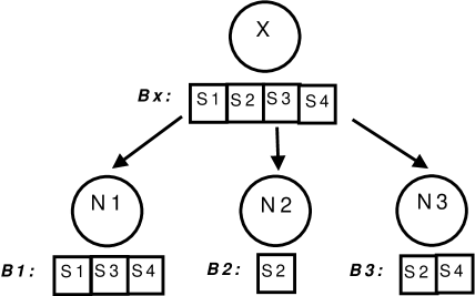
Figure 1: An example of a network, in which node ${\bf X}$ has to make coding decisions based on the buffer state of ${\bf 3}$ neighbors: ${\bf N_{1}}$, ${\bf N_{2}}$ and ${\bf N_{3}}$. For each neighbor, the figure depicts only that part of the buffer which contains symbols that are also stored in the buffer of node ${\bf X}$.

The ideas behind the algorithm are best described by the example shown in Fig. 1. Node $X$ (the node performing the coding algorithm) has in its buffer symbols $s_{1}$, $s_{2}$, $s_{3}$ and $s_{4}$. From Fig. 1 it is clear that some of these symbols can also be found in the buffers of the three neighbors of $X$. It follows that there are only two possible output packets which are optimal in the sense that they maximize the number of neighbors able to recover a new symbol immediately upon reception: $p=s_{1}\oplus s_{2}$ or $p=s_{2}\oplus s_{3}$. In both these cases, all neighbors are able to recover a new symbol from the received packet, since they have one and only one of the symbols therein. Moreover, no other combination of symbols can provide a packet that immediately provides a new symbol to every neighbor.

We now analyze the behavior of the Opportunistic algorithm. The initial set $S$ (from which we can choose a symbol to be mixed in the packet) is $S=\{s_{1},s_{2},s_{3},s_{4}\}$, due to the fact that none of the neighbors has recovered all the symbols in the buffer of node $X$. Thus, in the first iteration, each symbol in $S$ can be chosen with probability $1/4$. Suppose that the algorithm chooses $s^{*}=s_{1}$ (again with probability $1/4$). Then, we have that $C=\{s_{1}\}$ and $R(C)=\{N_{2},N_{3}\}$. Recall that $R(C)$ is the set of neighbors that have recovered all but one of the symbols in $C$ (in this case, it is the set of neighbors who have not yet recovered symbol $s_{1}$). Since $S$ is the set of symbols that (a) all the neighbors in $R(C)$ have already recovered and (b) have not yet been chosen, we have that $S=\{s_{2}\}$. In the second iteration, since $S=\{s_{2}\}$, the algorithm chooses $s^{*}=s_{2}$ and sets $C=\{s_{1},s_{2}\}$. Thus, $R(C)$ is equivalent to the entire set of neighbors and, since there are no more symbols recovered by the ensemble of neighboring nodes, we have that $S=\emptyset$. Hence, the algorithm stops and outputs the packet $p=s_{1}\oplus s_{2}$, which can be classified as an ideal packet.

We have seen that the algorithm outputs an ideal packet if the first chosen symbol corresponds to $s_{1}$ (and that this happens with probability $1/4$). Analogously, if the algorithm chooses $s_{3}$ first, then $C=\{s_{3}\}$ and $R(C)=\{N_{2},N_{3}\}$, yielding $S=\{s_{2}\}$. Hence, in the next step the algorithm chooses symbol $s_{2}$ which will lead to $S=\emptyset$. It follows that if the algorithm starts by choosing symbol $s_{3}$, then we get the ideal output packet $p=s_{2}\oplus s_{3}$.

Suppose now that the algorithm starts by choosing symbol $s_{2}$. In this case, we have that $C=\{s_{2}\}$ and $R(C)=\{N_{1}\}$. Since $S$ is the set of unselected symbols recovered by the ensemble of neighbors in $R(C)$, we have that $S=\{s_{1},s_{3},s_{4}\}$. Hence, in the second iteration, the algorithm has a probability $1/3$ of choosing each of the symbols in $S$. If the algorithm chooses symbol $s_{1}$ (respectively, symbol $s_{3}$), based on the same arguments as in the previous cases, we deduce that the output packet will be $p=s_{1}\oplus s_{2}$ (respectively, $p=s_{2}\oplus s_{3}$), which is an ideal packet. In case the algorithm chooses $s_{4}$, the output will not be an ideal packet. Thus, the probability that the algorithm outputs an ideal packet is given

$$\frac{1}{4}+\frac{1}{4}+\frac{1}{4}\left(\frac{1}{3}+\frac{1}{3}\right)=\frac{2}{3}.$$

It is worth noting that in this algorithm, the sole criterion for the choice of symbols to be mixed in the output packed is to ensure that a node which is able to recover a new symbol from the current set $C$ (constructed up to the given iteration), will continue to be able to recover a new symbol from the instances of $C$ that are constructed after that iteration. In other words, after the choice of the first symbol (which is performed randomly), the algorithm simply ensures that the number of neighbors that are able to recover a new symbol does not decrease with the next decisions.

III Optimized Coding Algorithms

In the following, we present two algorithms for the encoding process, both based on the knowledge of the recovery status of the neighboring nodes. In order to increase the speed of information dissemination, our algorithms make coding decisions that by design allow the neighboring nodes to recover another information unit immediately upon reception of a new coded packet.

III-A Greedy algorithm

The first algorithm gives priority to the symbols that are rarest within the neighborhood. The key is to find the combination of original symbols that maximizes the number of neighbors that are able to decode a new information unit.

Algorithm 2 Greedy algorithm

$\ \ \ \ \ \ \ \ C=\emptyset$
$\ \ \ \ \ \ \ \ \textrm{choose }s^{*}=\arg\max\limits_{s\in B_{x}}|R(\{s\})|$
$\ \ \ \ \ \ \ \ q=0$
$\ \ \ \ \ \ \ \ \textrm{while }|R(C\cup\{s^{*}\})|\geq q$
$\ \ \ \ \ \ \ \ \ \ \ \ \ \ \ \ q=|R(C\cup\{s^{*}\})|$
$\ \ \ \ \ \ \ \ \ \ \ \ \ \ \ \ \textrm{add }s^{*}\textrm{ to }C$
$\ \ \ \ \ \ \ \ \ \ \ \ \ \ \ \ \textrm{choose }s^{*}=\arg\max\limits_{s\in B_{x}\backslash C}|R(C\cup\{s\})|$
                end
$\ \ \ \ \ \ \ \ p=\bigoplus\limits_{s\in C}s$
                transmit $p$.

As shown in Algorithm 2, the choice of the first symbol is very different from the Opportunistic algorithm (Algorithm 1). Instead of a random choice, the Greedy algorithm selects the symbol that maximizes the number of nodes that are able to decode a new symbol if a packet of degree one is sent. This corresponds to maximizing $|R(\{s\})|$. If there are multiple symbols that satisfy this condition, the algorithm chooses one of them randomly. As we will see later on, a proper choice of the first symbol is crucial for a good performance. In fact, we will show that, if the nodes send packets of degree one (i.e. plain symbols) and use the selection criteria of our protocols, the resulting performance is already quite close to the performance of the Opportunistic algorithm.

Taking a closer look at the loop of this algorithm, we realize that after choosing the first symbol, the algorithm proceeds by selecting among the symbols yet to be chosen the element that maximizes the number of neighbors able to decode a new symbol from the packet, which is obtained by XORing this new symbol with all the symbols selected so far. This can be written as $|R(C\cup\{s\})|$. After choosing this candidate symbol (a symbol $s^{*}=\arg\max\limits_{s\in B_{x}\backslash C}|R(C\cup\{s\})|$), the algorithm will check if there is a gain in adding this candidate symbol to the set of symbols to be mixed in the output packet. Notice that, for the algorithm to continue, we do not require that neighbors that could previously recover a new symbol will continue to be able to do so; the algorithm continues as long as the number of neighbors able to recover a new symbol does not decrease from one step to the next one.

Denote by $p^{*}$ the packet obtained by XORing all the symbols chosen so far (i.e., all the symbols in the current set $C$) and denote by $s^{*}$ the candidate symbol. If the number of neighbors that are able to decode a new symbol from $p^{*}\oplus s^{*}$ (which is represented by $|R(C\cup\{s^{*}\})|$) is less than the number of neighbors that are able to decode a new symbol from $p^{*}$ (which is represented by $q$), i.e. if $|R(C\cup\{s^{*}\})|\geq q$, the algorithm stops and produces a packet that combines all of the symbols selected thus far.

Going back to the scenario illustrated in Fig. 1, we see that the algorithm starts by choosing the symbol $s^{*}$ that maximizes the size of $R(\{s\})$ over all $s$ in the buffer of node $X$, i.e. that maximizes the number of neighbors that do not have the symbol $s^{*}$. Clearly, $s^{*}$ is the rarest symbol in the neighborhood. It follows that the algorithm ends up choosing $s_{1}$ or $s_{3}$, since each of them is present in the buffer of only one of the neighbors. If the algorithm chooses symbol $s_{1}$, we have that $|R(\{s_{1}\})|=2$. In the first iteration, the algorithm sets $q=2$ and $C=\{s_{1}\}$. Next, the algorithm selects the symbol $s^{*}$ as the one that maximizes the size of $R(C\cup\{s\})$ over all $s\neq s_{1}$. More specifically, it will choose the symbol that maximizes the number of neighbors that are able to recover a new symbol from the packet obtained when XORing this candidate symbol with all the symbols in $C$. In this case, since $C=\{s_{1}\}$ and all $3$ neighbors can recover a new symbol from $s_{1}\oplus s_{2}$, this candidate symbol is $s^{*}=s_{2}$. Now, the algorithm checks if the number of neighbors that can recover a new symbol increases when compared to the previous step. In this case, since $q=2$ neighbors recovered a new symbol and adding the candidate symbol increases this number to $3$ (i.e. $|R(C\cup\{s_{2}\})|\geq 2$), the algorithm continues by updating $q$ to $q=3$ and adding the candidate symbol to the packet: $C=\{s_{1},s_{2}\}$. Now, the algorithm chooses the next candidate symbol using the same rule, i.e. to maximize the number of neighbors that are able to recover a new symbol. In this case, this symbol can be $s_{3}$ or $s_{4}$. In either case, we have that only one neighbor will be able to recover a new symbol if the candidate symbol is added, thus we will have $|R(C\cup\{s^{*}\})|=1$. In the subsequent step, since $|R(C\cup\{s^{*}\})|<3=q$, the algorithm stops and outputs the packet $p=s_{1}\oplus s_{2}$, which is an ideal packet.

Notice that in the first choice we had two options: $s_{1}$ and $s_{3}$. We saw that if $s_{1}$ is chosen, the algorithm outputs the ideal packet $p=s_{1}\oplus s_{2}$. Using analogous arguments, it is easy to see that if $s_{3}$ is chosen in the first step, the algorithm outputs the packet $p=s_{2}\oplus s_{3}$, which is also an ideal packet. Thus, we have that in this example, with probability $1$, the Greedy algorithm outputs an ideal packet.

Similarly to the Opportunistic algorithm, the Greedy algorithm evolves in each iteration by selecting a symbol to be added to the set of symbols that will form the output packet. After the choice of the first symbol, the algorithm ensures that the number of neighbors that are able to decode new symbols does not decrease with the next decisions. Beyond the choice of the first symbol (which has a significant impact on the performance as we will see latter on), the selection procedure targets the symbol that will maximize the number of neighbors that are able to decode, whereas the Opportunistic algorithm make this selection in a purely random fashion.

III-B Equalizing algorithm

The Greedy algorithm presented in the previous section is prone to lead to an uneven distribution of information. In the worst case, some nodes that are not well connected to the rest of the network might receive mostly packets they cannot decode, since they lack some of the information units that all the other nodes already have. These nodes would be served by the greedy algorithm only after all other nodes have decoded all of the information, leading to a high worst case delay. The way to prevent this from happening is to equalize the recovery level among the neighbors instead of maximizing it in a greedy fashion.

The so called Equalizing algorithm pursues mainly the goal of giving new decodable information to the neighbors that have recovered the fewest information units, thus increasing the minimum number of recovered packets per node.

Algorithm 3 Equalizing algorithm

$\ \ \ \ \ \ \ \ C=\emptyset$
$\ \ \ \ \ \ \ \ B=B_{x}$
$\ \ \ \ \ \ \ \ R^{*}(C)=\{j:C\subseteq B_{j}\}$
$\ \ \ \ \ \ \ \ \textrm{while }|B|>0\textrm{ and }|R^{*}(C)|>0$
$\ \ \ \ \ \ \ \ \ \ \ \ \ \ \ \ \textrm{choose }J=\arg\min\limits_{j\in R^{*}(C)}|B_{j}|$
$\ \ \ \ \ \ \ \ \ \ \ \ \ \ \ \ S=B\cap\overline{B}_{J}$
$\ \ \ \ \ \ \ \ \ \ \ \ \ \ \ \ \textrm{choose }s^{*}=\arg\max\limits_{s\in S}|R(C\cup\{s\})|$
$\ \ \ \ \ \ \ \ \ \ \ \ \ \ \ \ \textrm{add }s^{*}\textrm{ to }C$
$\ \ \ \ \ \ \ \ \ \ \ \ \ \ \ \ B=B\cap B_{J}$
                end
$\ \ \ \ \ \ \ \ p=\bigoplus\limits_{s\in C}s$
                transmit $p$.

IN Algorithm 3, $R^{*}(C)=\{j:C\subseteq B_{j}\}$ represents the set of neighbors that have all the symbols in $C$. In each step, the algorithm chooses the neighbor that has the least recovered packets among those not yet considered. Then, the algorithm selects one of the symbols that this particular neighbor has not yet recovered (and that all the previously chosen neighbors did recover, thus ensuring that the previously chosen neighbors can still decode the packet). This symbol is added to the packet to be sent.

The algorithm needs to keep track of the symbols that neighbors chosen so far have already recovered. This is captured by set $B$. One condition to stop the loop of the algorithm is precisely the existence of symbols in $B$. If there are no symbols $B$, i.e. if there is no symbol that has been recovered by all the nodes chosen up to a certain iteration, no symbol can be added to the packet to be sent without rendering at least one of the neighbors unable to decode. The other condition for the loop to stop is $|R^{*}(C)|>0$, which means that the loop only continues if there are still neighbors that have recovered all the symbols in the output packet constructed so far. If there are no neighbors in this condition, no further nodes will be able to recover a new symbol irrespective of which symbol is added to the packet.

In each iteration, the algorithm starts by inspecting all nodes that have recovered all the symbols in the packet constructed so far (i.e. neighbors in $R^{*}(C)$ which implies that no neighbor can be chosen twice) and finding the one that recovered the least number of symbols. More specifically, we choose the neighbor $J$ that satisfies $J=\arg\min\limits_{j\in R^{*}(C)}|B_{j}|$. After making this selection, the algorithm calculates the set of symbols that can still be added to the packet. These symbols must have been recovered by all the previously chosen neighbors(i.e., symbols in $R$) and cannot have been recovered by the neighbor that was chosen in the current iteration (i.e., symbols not in $B_{J}$). Thus, the set of candidates is defined by $S=R\cap\overline{B}_{J}$.

Next, from this set of candidate symbols, the algorithm selects the one that maximizes the number of neighbors that are able to decode a new symbol, assuming that the output packet results from the XOR of all symbols in $C$. After this choice, the algorithm adds the symbol to the set $C$ and updates the set $R$. The new set $R$ will be the set of symbols shared by all the neighbors that were chosen before the current iteration (namely $R$) and possessed by the new chosen neighbor ($B_{J}$), i.e. $R=R\cap B_{J}$. When the loop is completed, the algorithm computes the packet to be sent by XORing all the symbols in $C$.

Once again, we will use the scenario in Fig. 1 to clarify the main steps of the algorithm. The algorithm starts by setting $C=\emptyset$, $B=\{s_{1},s_{2},s_{3},s_{4}\}$ and $R^{*}(C)=\{N_{1},N_{2},N_{3}\}$ (recall that $R^{*}(C)$ represents the set of neighbors that have already recovered all of the symbols in $C$). In the first iteration, the algorithm starts by checking which neighbor has the smallest buffer, i.e. the one with the smallest number of recovered symbols. In this case, the chosen neighbor is $N_{2}$, since it only recovered symbol $s_{2}$. Then, the algorithm computes the set of symbols that this node does not have in its buffer: $s=\{s_{1},s_{3},s_{4}\}$. The goal is to provide a new symbol to this particular neighbor. Hence, the first chosen symbol is a symbol from $S$ and, since we also want to provide (if possible) new symbols to other neighbors, the algorithm chooses the symbol that is more rare within the neighborhood, among all the symbols in $S$. In this case, we have two options: $s_{1}$ or $s_{3}$. Suppose that the algorithm chooses $s^{*}=s_{1}$. We have that $C=\{s_{1}\}$ and $B=\{s_{2}\}$, i.e. $B$ is the set of symbols that node $N_{2}$ has already recovered. It is necessary to keep track of the symbols that all the neighbors chosen by the algorithm have already recovered to ensure that the neighbors with the smaller number of recovered symbols will be able to recover a new symbol from the resulting output packet.

Next, in the second iteration, the algorithm chooses the neighbor that has the smallest number of recovered symbols among all the neighbors that have all the symbols in the current instance of set $C$, i.e. among the neighbors in $R^{*}(C)$. In this case, $R^{*}(C)=\{N_{1}\}$ and thus the chosen neighbor is $N_{1}$. Now, the set of symbols that can be added to $C$ is the set of all symbols that all the previously chosen neighbors have in their buffers, $B$, and that the neighbor chosen in the current iteration does not have in its buffer, $\overline{B}_{1}$. Thus, in this case, we have that $S=\{s_{2}\}$ and, hence, $C=\{s_{1},s_{2}\}$. Notice that there are no further symbols that have been recovered by all the chosen neighbors, i.e. $B=\{s_{2}\}\cap\{s_{1},s_{3},s_{4}\}=\emptyset$. Thus, the algorithm cannot continue and consequently outputs the packet $p=s_{1}\oplus s_{2}$, which is an ideal packet.

In the first iteration, we could have chosen symbol $s_{3}$ instead of $s_{1}$. Using similar arguments, it is easy to see that, if $s_{3}$ is chosen, the algorithm outputs the packet $p=s_{2}\oplus s_{3}$, which is also an ideal packet. Therefore, we again have that with probability $1$ the Equalizing algorithm outputs an ideal packet in our example.

IV Simulation Results

In this section we present and discuss the performance of the aforementioned coding algorithms in various scenarios. The main part of the analysis assumes the simple decoding algorithm.

We discuss the enhancement of performance provided by the use of a full decoding scheme at the end of this section. The following performance metrics are of interest for the analysis of the algorithms. The recovery rate of a node is the number of original packets recovered by the node as a function of the total number of packets received by the node. It measures the speed of the dissemination process and thus the overall efficiency of the protocol. This metric is crucial in communication networks, especially for delay-sensitive applications such as real-time media streaming, where the disseminated segments must be recovered by the receivers within strict time intervals. We average the recovery rates over all nodes and repeated the simulations several times so as to get tight confidence intervals. For the recovery rate shown in the next plots, the confidence intervals are all within $\pm 2\%$. These intervals are omitted from the figures for the sake of readability.

The codeword degree is measured as the number of original symbols which are combined to form a (coded) packet and we calculate the average codeword degree over all nodes. For the analysis of the single-hop scenario we also consider packet delay as defined in Definition 2 of [10]. The delay that a receiver experiences is the total number of received packets that do not allow immediate recovery of a new original symbol. Again we consider this delay averaged over all nodes. Finally, the information potential is the number of original symbols that are available at a given neighboring node, but not at the node itself. This metric is useful for analyzing the overlap between the information recovered by a target node and by its neighbors. It provides a measure of the efficiency of the coding process and gives an insight into the degree of freedom available for making coding decisions.

The simulation results have been obtained using a custom C++ simulator. It provides an ideal (collision-free) MAC layer, with a sequential or random scheduling of packets. All transmissions use physical layer broadcast.

IV-A Single-hop Scenario

In this setting, a single source node broadcasts $100$ original symbols to its $100$ neighbors over independent erasure channels and, as in [10], perfect feedback is available from the receivers to the source. For all the algorithms in our analysis, i.e. Greedy, Equalizing, Opportunistic and ANC, the source node starts by sending out all the original symbols in uncoded form. It is only after this initial stage that the source node sends encodings of the original symbols as described in Sections II and III. The erasure probability is set to $0.5$.

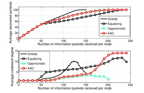
Figure 2: Recovery rate (top) and average codeword degree (bottom) for the single-hop scenario.

In Fig. 2, the Greedy algorithm shows the best performance in the single-hop scenario. With this algorithm, all nodes achieve the full recovery of the $100$ original symbols within $150$ information packets received. From the first 100 uncoded packets the receivers miss around 50 original packets and they differ from node to node due to the random erasure pattern. This allows the Greedy algorithm to increase the degree of the coded packets compared to the Opportunistic and ANC algorithms between 50 received packets and 120 received packets. When the process approaches the full recovery state, the number of nodes still missing some packets decreases and low degree codewords are sufficient to serve these nodes. Given the diversity of missing information among all the receivers and the large amount of information potential of the neighbors (due to the erasure pattern), the degree of freedom for making coding decisions lets the source node perform the coding that best allows a large number of receivers to immediately recover a new symbol from the sent packet.

The Equalizing algorithm has a considerably worse recovery rate than the other algorithms. The reason is visible in Fig. 2, bottom, where Equalizing starts using higher and higher codeword degrees quite early on. Since it is designed to provide an immediately decodable packet to the neighbor(s) which recovered the least number of original symbols, many other neighbors are not able to decode the packet — their composition of recovered packets differs from those poor nodes. Focusing only on the poor nodes results in a packet that despite its high degree is useful only for few receivers.

Surprisingly, the performance of ANC and of the Opportunistic algorithm is almost the same for most of the simulation. The Opportunistic algorithm, which allows the source node to use the neighborhood status information to make the coding decisions, performs just slightly better than ANC. Due to the large information potential of the neighbors and to the huge diversity of missing information among the receivers, the choice of which symbols to encode is not crucial, as long as the number of symbols that are combined is the same. Only at the very end, the information obtained from the receivers by the Opportunistic algorithm allows the source node to send the last few missing symbols without wasting time sending packets that carry encodings of randomly picked symbols.

Focusing the analysis on the packet delay, we note that the Greedy algorithm achieves the lowest packets delay of only $30$ not useful packets (averaged over all receivers), followed by the Opportunistic algorithm with $75$, ANC with $90$ and Equalizing with $100$, as could be expected from the previous analysis.

IV-B Multi-hop Scenario

In the multi-hop scenarios, each of the $100$ nodes generates one original symbol that is intended to be delivered to every other node in the network.

IV-B1 Static grid

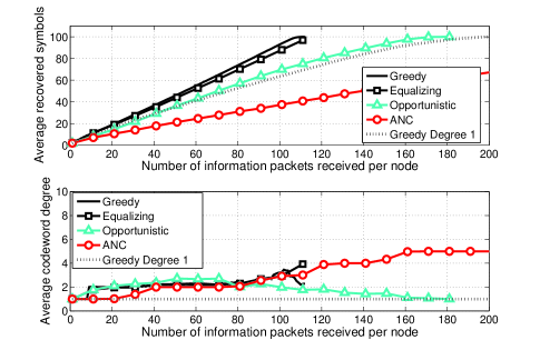
Figure 3: Recovery rate (top) and average codeword degree (bottom) for 100 nodes on a static grid.

In this setting, nodes are placed on a static grid (that wraps around) and each node has eight neighbors to communicate with. In Fig. 3, top, the algorithm with the best performance is the Greedy one (as in the previous scenario), but now the difference to the performance of the Equalizing algorithm is much smaller. From the analysis of their respective average codeword degrees, in Fig. 3, bottom, we see that the coding degree of our two algorithms is very similar, except for the very end where the Equalizing algorithm takes longer than the Greedy algorithm to increase the coding degree for recovery of the last missing symbols.

The high degree of correlation of the information recovered by the neighbors, due to the wrap around and the symmetrical topology, and the consequently minor diversity of information stored by the neighbors compared to the single-hop setting, makes the use of packets with high degree ineffective. Moreover, choosing which original packets to combine has a huge impact on the performance of the dissemination process. To visualize this, we also show the recovery rates achieved by the algorithms corresponding to Greedy and Equalizing when we limit the codeword degree to one, i.e., only an uncoded packet is sent. In the top graph of Fig. 3, we plot only Greedy with codeword degree one, but both of the algorithms perform the same. Even in this limited case, the recovery rates of our algorithms are very close to the recovery rate of the Opportunistic algorithm with coding. The few degrees of freedom for making coding decisions, typical of this setting, limit the performance of the Opportunistic algorithm, where the first symbol is chosen randomly.

Finally, the impact of using neighborhood recovery status in the coding decisions is obvious when we compare the recovery rate of the ANC algorithm with the recovery rates of the other algorithms. For instance, the total number of received packets necessary to achieve full recovery is, in the case of ANC, several times larger than in the case of Greedy, while the average codeword degree is quite similar for most of the values of received packets.

IV-B2 Static random and clustered networks

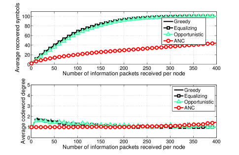
Figure 4: Recovery rate (top) and average codeword degree (bottom) for the static random network, 100 nodes.

In this section, we consider two different scenarios: static random topologies with an average density of 8 nodes per communication range, and clustered networks. These static networks are relatively sparse, which means that the information potential of neighbors is smaller than in the grid network and that the diversity of information stored by the neighbors is lower. The high degree of correlation among the original symbols recovered by the nodes explains why the Greedy, Equalizing and Opportunistic algorithms perform similarly (Fig. 4). No degree of freedom for making specific coding decisions is left to these algorithms, so that the differences are small. Also in such settings, ANC cannot perform well given the extremely low level of diversity of information among nodes. In Fig. 5, top, we show the low information potential. Only Greedy and Equalizing increase the diversity of information among neighbors at the beginning of the simulations, as expected from the description of their coding mechanism in Section III. After  $75$ packets received, all algorithms experience the same neighborhood information potential (due to the natural progressive lowering of the diversity of information over time). The differences of the performance in terms of recovery rate, among Greedy, Equalizing and Opportunistic algorithms increase slightly for larger node densities (not shown here). Such settings are closer to the characteristics of a grid topology concerning the degrees of freedom for making coding decisions.

The delay experienced by nodes using the Greedy and Equalizing algorithms in static sparse random and clustered networks shows an interesting result. For each setting in analysis, the average delay is practically the same for the two algorithms, however the worst delay (i.e. the delay experienced by the node with the highest delay) of the Greedy algorithm is up to $5$% higher than the worst delay of the Equalizing algorithm. Since the Equalizing algorithm will always try to provide an immediately decodable packet to the neighbor with the lowest number of recovered original symbols, this will obviously improve worst case delay.

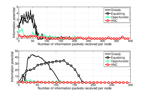
Figure 5: Neighborhood information potential for static random network (top) and moderate mobility scenario (bottom).

IV-B3 Moderate mobility

In this scenario, we consider nodes moving according to a random waypoint mobility model with speeds uniformly distributed in the interval $[2,4]\>m/s$. Again, the node density allows on average for eight neighbors per node. We assume perfect information about the neighbor recovery status.

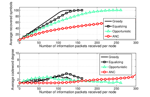
Figure 6: Recovery rate (top) and average codeword degree (bottom) for the mobile scenario, 100 nodes.

In Fig. 6, top, we notice that the performance of the algorithms under consideration in terms of recovery rate is somewhat similar to the one observed in the static grid setting (Fig. 3). Due to the mobility of the nodes, the correlation among the original symbols recovered by neighbors is much lower in the case of moderate mobility than in the case of a static grid or static random networks. An insight into the differences of information potential of neighbors for two extreme cases is given in Fig. 5: on the top the random static network shows a lower diversity of information among neighbors than in the mobile case, bottom, where the information potential with our algorithms can achieve very high values of up to $40-50$, whereas for the other protocols the measured values are close to $0$. As seen in the previous section, our algorithms allow nodes to maintain a high diversity of information in the neighborhood and thus a high degree of freedom for the coding decisions.

It is also important to notice that the coding degree of the Equalizing algorithm is always higher than the coding degree of the Greedy algorithm. This observation and the fact that the recovery rate of the Greedy algorithm is higher than the recovery rate of the Equalizing algorithm let us conclude that the Equalizing algorithm builds packets with a too high codeword degree, rendering these packets not immediately decodable. We will see later on in this paper that, if we allow the use of a full decoding process, i.e., all the packets in the buffer (decoded and undecoded) are considered for the decoding algorithm, the recovery rate of the Equalizing algorithm can actually surpass the recovery rate of the Greedy algorithm.

IV-C Performance gains using a complete buffer decoding mechanism

In this section, we investigate the benefits of full decoding, which is more efficient (in the sense that it does not discard useful packets) but also more costly in terms of energy, memory requirements, and processing. Up to now, we were considering a scheme were only the immediately recovered original symbols were considered for the simple decoding process. Here, all the packets received (decoded and undecoded) are taken into consideration when performing the decoding of the received packets. In the following figures, we omit the plot of the average codeword degree for the sake of readability of the recovery rate. Also, the average codeword degree of the algorithms using a full decoding scheme is almost the same as the one with the simple decoder, except for a slight increase of the average codeword degree.

As we already mentioned in the previous analysis, it is expected that the recovery rate significantly increases with the full decoding scheme, since the algorithms often produce packets that are not immediately decodable for some neighbors but that are innovative. The node is not able to recover a new original symbol from the received information packet since it did not yet recover the required other original symbols that form the coded information packet. By storing these not immediately decodable but innovative packets in the buffers and considering these packets in the decoding process, nodes can find these packets helpful later on, when more and more (innovative or immediately decodable) packets are received, increasing the recovery rate of the algorithm. This benefit can be observed in Fig. 7, where the recovery rate of the algorithms using a full decoding mechanism (including the Systematic Random Network Coding algorithm) is plotted for the single-hop scenario.

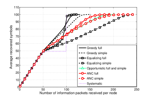
Figure 7: Recovery rate for the single-hop scenario with simple and full decoding schemes.

Comparing the results obtained with this full decoding scheme to the results obtained with a simple decoding scheme, we can observe a major improvement of the recovery rate of the Equalizing algorithm. With the full decoding scheme, the Equalizing algorithm has a recovery rate that slowly increases after the initial phase (where the nodes first send the original symbols uncoded once) and, at around $80$ packets received, shows a “smooth” step behavior that is typical of the random network coding algorithms (e.g. Systematic Random Network Coding). The Equalizing algorithm reaches the full recovery state before the Greedy algorithm. However, the recovery rate of the Greedy algorithm is higher than the one of the Equalizing algorithm before the step behavior takes place.

We also consider the packet delay when using a full decoding mechanism. The delay presented by Greedy with this decoding scheme is $10$ lower than the delay obtained when using the simple decoder, with a total averaged delay of $20$. In [10], none of the algorithms proposed for the single-hop scenario is able to achieve such a low delay (in the same conditions as used here). The Equalizing algorithm experiences only an average delay of $40$ packets, ANC of $70$ and the Systematic Random Network Coding of $50$ as in [10].

After analyzing the performance enhancements achieved by using a full decoding scheme in the single-hop scenario, we now discuss the results obtained for the multi-hop scenario with moderate mobility. We have chosen this particular setting of the multi-hop scenario because the performance of the algorithms in the other settings is similar to the one presented in Fig. 3, although there are some differences that should be pointed out. With a full decoding scheme, the Greedy and Equalizing algorithms have quite similar performance. Moreover, the enhancements achieved by the other algorithms when using a full decoding scheme are negligible except for the ANC algorithm, for which the performance is still far from the performance achieve by our algorithms.

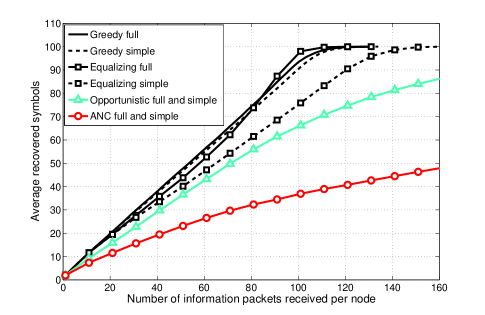
Figure 8: Recovery rate for the multi-hop mobile network, with simple and full decoding schemes.

In Fig. 8, we can again see that in the moderate mobility scenario and with a full decoding scheme, there is a major improvement of performance of the Equalizing algorithm. The recovery rate of the Equalizing algorithm comes very close to the recovery rate of the Greedy algorithm until around $80$ packets received (similar to the behavior in the single-hop scenario). After this value, the Equalizing algorithm is faster in recovering new original packets, reaching the full recovery state $10$ packets before the Greedy algorithm. It is also interesting to notice that there is no significant difference in terms of recovery rate between the two decoding mechanisms in combination with the Greedy algorithm. This behavior was expected, since the Greedy algorithm was designed for immediate decoding. Few not immediately decodable packets mean that a complete buffer decoding mechanism can just slightly outperform a simple decoder.

V Conclusions

In this paper we proposed two coding algorithms which exploit feedback information on the recovery status of neighboring nodes. Through the analysis of a wide range of settings in our simulations, we show that the Greedy algorithm consistently outperforms all other algorithms in terms of number of immediately decodable packets, which is fundamental for delay-sensitive applications in wireless networks such as real-time media streaming. Moreover, satisfactory results of the Greedy algorithm are already obtained using just a simple decoder, whereas for the Equalizing algorithm the use of Gaussian elimination improves the performance significantly. However, using the Equalizing algorithm is beneficial in some inhomogeneous (clustered) topologies, where the worst case delay is lower than that of the Greedy algorithm at a similar recovery rate.

The algorithms proposed in this paper focus on immediate decodability, and hence take the decoding delay as the sole optimization criterion. As a next step, we intend to explore the design tradeoff between delay and throughput in more detail. The perceived quality of a video transmissions is largely dependent on the right balance between the two. An algorithm which imposes slightly less stringent delay requirements and allows decoding after reception of a fixed number of packets (as opposed to just one packet), will provide higher throughput, which may improve the overall perceived quality. We further assumed instantaneous feedback in the evaluation of the algorithms. The analysis of the impact of imperfect and delayed feedback on the performance of network coding algorithms is left as an important item for future work.

References

- [1] R. Ahlswede, N. Cai, S.-Y. Li, and R. Yeung, “Network information flow,” IEEE Trans. on Information Theory, vol. 46, no. 4, pp. 1204–1216, July 2000.
- [2] P. A. Chou, T. Wu, and K. Jain, “Practical network coding,” in 41st Allerton Conf. Communication, Control and Computing, Monticello, IL, US, Oct. 2003.
- [3] C. Fragouli, J.-Y. L. Boudec, and J. Widmer, “Network coding: An instant primer,” ACM Computer Communication Review, Jan. 2006.
- [4] A. Albanese, J. Blomer, J. Edmonds, M. Luby, and M. Sudan, “Priority encoding transmission,” IEEE Transactions on Information Theory, vol. 42, no. 6, pp. 1737–1744, 1996.
- [5] A. Shokrollahi, “Raptor codes,” IEEE/ACM Transactions on Networking (TON), vol. 14, pp. 2551–2567, 2006.
- [6] S. Sanghavi and M. LIDS, “Intermediate Performance of Rateless Codes,” in Proceedings of the IEEE Information Theory Workshop, Tahoe City, CA, September 2007.
- [7] A. Kamra, V. Misra, J. Feldman, and D. Rubenstein, “Growth Codes: Maximizing Sensor Network Data Persistence,” in ACM SIGCOMM, Pisa, Italy, Sep. 2006.
- [8] D. Munaretto, J. Widmer, M. Rossi, and M. Zorzi, “Resilient Coding Algorithms for Sensor Network Data Persistence,” in 5th European Conference on Wireless Sensor Networks, EWSN 2008, Bologna, Italy, Jan.-Feb. 2008.
- [9] S. Katti, H. Rahul, W. Huss, D. Katabi, M. Medard, and J. Crowcroft, “XORs in The Air: Practical Wireless Network Coding,” in ACM SIGCOMM, Pisa, Italy, Sep. 2006.
- [10] L. Keller, E. Drinea, and C. Fragouli, “Online Broadcasting with Network Coding,” in 4th Workshop on Network Coding, Theory, and Applications, NetCod 2008, Hong Kong, China, Jan. 2008.
- [11] T. Ho, R. Koetter, M. Medard, D. R. Kerger, and M. Effros, “The benefits of coding over routing in a randomized setting,” in Proc. of the IEEE International Symposium on Information Theory (ISIT), Yokohama, Japan, June/July 2003.
- [12] D. Munaretto, J. Widmer, M. Rossi, and M. Zorzi, “Network coding strategies for data persistence in static and mobile sensor networks,” in International Workshop on Wireless Networks: Communication, Cooperation and Competition (WCN3 2007), Limassol, Cyprus, Apr. 2007. [Online]. Available: http://icapeople.epfl.ch/widmer/files/Munaretto2007Persistence.pdf