Evaluation of mutual information estimators on nonlinear dynamic systems

Abstract

Mutual information is a nonlinear measure used in time series analysis in order to measure the linear and non-linear correlations at any lag $\tau$. The aim of this study is to evaluate some of the most commonly used mutual information estimators, i.e. estimators based on histograms (with fixed or adaptive bin size), $k$-nearest neighbors and kernels. We assess the accuracy of the estimators by Monte-Carlo simulations on time series from nonlinear dynamical systems of varying complexity. As the true mutual information is generally unknown, we investigate the existence and rate of consistency of the estimators (convergence to a stable value with the increase of time series length), and the degree of deviation among the estimators. The results show that the $k$-nearest neighbor estimator is the most stable and less affected by the method-specific parameter.

I Introduction

Mutual information is a popular nonlinear measure of time series analysis, best known as a criterion to select the appropriate delay for state space reconstruction Kantz and Schreiber (1997). It is also used to discriminate different regimes of nonlinear systems Chillemi et al. (2003); Wicks et al. (2007) and to detect phase synchronization Schmid et al. (2004); Kreuz et al. (2007). Besides nonlinear dynamics, it is used in various statistical settings, mainly as a distance or correlation measure in data mining, e.g. in independent component analysis and feature-based clustering Tourassi et al. (2001); Priness et al. (2007).

It is well-known that any estimate of mutual information, either between two variables or as a function of delay for time series, is (almost always) positively biased Treves and Panzeri (1995); Moddemeijer (1989); Paninski (2003). For numerical-valued variables and time series, the mutual information increases with finer partition depending on the underlying distribution or process and the sample size. Beyond the classical histogram-based partitioning, other schemes have been used to estimate the densities inherent in the measure of mutual information, e.g. using kernels and $k$-nearest neighbors Moon et al. (1995); Kraskov et al. (2004).

Although there are some works comparing mutual information estimators in Moon et al. (1995); Darbellay and Vajda (1999); Steuer et al. (2002); Daub et al. (2004); Kraskov et al. (2004); Cellucci et al. (2005); Nicolaou and Nasuto (2005); Trappenberg et al. (2006); Khan et al. (2007), to the best of our knowledge, there has not been a comparison of all commonly used estimators, including the selection of their parameters, on time series from dynamical deterministic systems.

Moon et al. Moon et al. (1995) developed a kernel mutual information estimator, as an extension of Silverman’s work Silverman (1986). This estimator is compared to the locally adaptive histogram-based estimator of Fraser and Swinney Fraser and Swinney (1986) on four linear and nonlinear systems using as a performance criterion the lag of the first minimum of mutual information. Darbellay and Vajda Darbellay and Vajda (1999) suggested an adaptive histogram-based estimator and compared it with mutual information estimators derived from maximum likelihood estimators for some bivariate distributions with analytically known mutual information. Steuer et al. Steuer et al. (2002) presented three histogram-based estimators, investigated their bias and suggested using the kernel estimator. Daub et al. Daub et al. (2004) estimated mutual information using B-spline functions and compared it to an entropy estimator suggested by Paninski Paninski (2003) and a kernel density estimator on data sets drawn from a known distribution. They claimed that their method is computationally faster than the kernel estimator and improves the simple binning method. Kraskov et al. Kraskov et al. (2004) developed an estimator of mutual information based on $k$-nearest neighbors and compared it to the adaptive histogram-based estimator of Darbellay and Vajda but only on Gaussian and some non-Gaussian distributions with analytically known mutual information. In Cellucci et al. (2005), equidistant and equiprobable histogram-based estimators (using three selection criteria for the number of bins $b$) are compared to the algorithm of Fraser and Swinney on nonlinear systems as to their robustness in detecting a fixed delay for the first minimum of the mutual information (similarly to Moon et al. (1995)). They also use the bias as a performance criterion in the case of Gaussian processes (where the true mutual information is known) and find that the equiprobable histogram-based estimator is more accurate and the Fraser and Swinney estimator is computationally ineffective.

In a different setting, in Nicolaou and Nasuto (2005) the estimators of equidistant histograms, kernels, B-splines, and $k$-nearest neighbors, are tested on electroencephalographic data from rats in order to find dependencies between left and right channels. Using the surrogate data test for the significance of dependence and bootstrap confidence intervals for the estimators, they concluded that the B-spline estimator is largely affected by its parameter and the $k$-nearest neighbor is the most consistent and less dependent on its parameter. Trappenberg et al. Trappenberg et al. (2006) compared the equidistant histogram-based method, the adaptive histogram-based method of Darbellay and Vajda and the Gram-Charlier polynomial expansion Blinnikiov and Moessner (1998) and concluded that all three estimators gave reasonable estimates of the theoretical mutual information, but the adaptive histogram-based method converged faster with the sample size. A more comprehensive evaluation of mutual information estimators including the kernel, $k$-nearest neighbor, equiprobable histogram-based estimators and an estimator using the Edgeworth approximation to estimate densities, was recently presented in Khan et al. (2007), focusing on the deviation of the mutual information from a linear correlation measure on linear and nonlinear time series (using the Henon map for the chaotic case). In the same paper, a small scale simulation showed dependence of the performance of the kernel and nearest neighbor estimators on their parameter.

Given the varying results in the literature on the different mutual information estimators, we study here the performance of three commonly used estimators, i.e. estimators based on histograms (with fixed or adaptive bin size), $k$-nearest neighbors and kernels, on time series from nonlinear deterministic systems. Moreover, we investigate the optimal parameter for the determination of the two-dimensional partitioning for each method. Monte-Carlo simulations of dynamical systems of varying complexity and observational noise level are used in order to assess the accuracy of the estimators. Commonly used parameter selection methods are considered for all but the kernel estimators, where a range of bandwidths are tested.

The structure of the paper is as follows. In Section II the estimators considered in this study are presented. In Section III the results of the simulations are presented and in Section IV the results are discussed and conclusions are drawn.

II Estimators of mutual information

In information theory, mutual information is defined as a measure of mutual dependence of two variables $X$ and $Y$ and has the form

$$\mathbf{I}(X,Y)=\int_{X}\int_{Y}f_{X,Y}(x,y)\log_{a}{\frac{f_{X,Y}(x,y)}{f_{X}(x)f_{Y}(y)}}\mbox{d}x\mbox{d}y$$ (1)

where $f_{X,Y}(x,y)$ is the joint probability density function (pdf) of $X$ and $Y$, and $f_{X}(x)$, $f_{Y}(y)$ are the marginal pdfs of $X$ and $Y$, respectively. The units of information of $I(X,Y)$ depend on the base of the logarithm, e.g. bits for the base of $2$ and nats for the natural logarithm in (1).

Assuming a partition of the domain of $X$ and $Y$ the double integral becomes a sum over the cells of the two-dimensional partition:

$$\mathbf{I}(X,Y)=\sum_{i,j}p_{X,Y}(i,j)\log_{a}{\frac{p_{X,Y}(i,j)}{p_{X}(i)p_{Y}(j)}}$$ (2)

where $p_{X}(i)$, $p_{Y}(j)$, and $p_{X,Y}(i,j)$ are the marginal and joint probability distributions over the elements of the partition. In the limit of fine partitioning the expression in (2) converges to (1). This may partly justify the abuse of notation of mutual information for the continuous and the discretized variables.

It is always $\mathbf{I}(X,Y)\geq 0$, with equality holding for independent variables, and $\mathbf{I}(X,Y)\leq H(X)\leq\log_{a}{n}$ (Jensen inequality), where $H(X)=-\sum_{i=1}^{n}p(x_{i})\log_{a}{{1}/{p(x_{i})}}$ is the entropy of $X$. We do not discuss the mutual information in terms of entropies as the estimation of mutual information we study in this work boils down to the estimation of the densities in (1) or probabilities in (2).

For a time series $\{X_{t}\}_{t=1}^{n}$, sampled at fixed times $\tau_{s}$, the mutual information is defined as a function of the delay $\tau$ assuming the two variables $X=X_{t}$ and $Y=X_{t-\tau}$, i.e. $\mathbf{I}(\tau)=\mathbf{I}(X_{t},X_{t-\tau})$.

The true mutual information is generally not known as joint and marginal probability density functions are unknown. A different estimator $I(\tau)$ of $\mathbf{I}(\tau)$ is determined from the way the theoretical densities in (1) or probabilities in (2) are estimated. We discuss below three estimators considered in this work and their dependency on a parameter inherent in the estimation of the densities or probabilities.

II.1 Histogram-based estimators

The naive histogram-based estimator regards a partition of the range of values of each variable into $b$ discrete bins of equal length, termed as equidistant partitioning (ED). The density at each bin and each two-dimensional cell, or rather the probability functions in (2), are estimated by the corresponding relative frequency of occurrence of samples in the bin or cell. Many different criteria have been developed for the selection of the number of bins $b$ or equivalently the length of each bin, e.g. see Bendat and Piersol (1966); Duda and Hart (1973); Scott (1992); Knuth (2006). Alternatively, the partition can be done into equiprobable bins, so that each bin has the same occupancy, termed as equiprobable partitioning (EP). In any case the partitioning is the same for both variables and the only free parameter is $b$. A number of criteria for selecting $b$ for one-dimensional binning can been used and in Cellucci et al. (2005) the Cochran condition (requiring at least 5 samples in a bin) extended for two-dimensional cells is used to select $b$.

An extension of the equidistant and equiprobable partitioning is the adaptive partitioning of the two-dimensional plane. Darbellay and Vajda built an algorithm to estimate the mutual information (AD) by calculating relative frequencies on appropriate partitions formed in a way that conditional independence is achieved on the cells Darbellay and Vajda (1999). The advantage of the estimator of Darbellay and Vajda is that it is adaptive to the data and does not involve a parameter for the binning. It does however involve a parameter for the independence test that can affect the performance of the estimator.

II.2 $k$-nearest neighbor estimator

Kraskov et al. proposed an estimator of mutual information that uses the distances of $k$-nearest neighbors to estimate the joint and marginal densities Kraskov et al. (2004) (KNN). For each reference point from the bivariate sample, a distance length is determined so that $k$ neighbors are within this distance length. Then the number of points with distance less than half of this length give the estimate of the joint density at this point and the respective neighbors in one-dimension give the estimate of the marginal density for each variable. The algorithm uses discs (or squares depending on the metric) of a size adapted locally and then uses the corresponding size in the marginal subspaces, so in some sense the estimator is data adaptive. However, it involves as a free parameter the number of neighbors $k$; large $k$ regards a small $b$ of the histogram-based estimator. However, the estimator does not use a fixed neighborhood size and therefore there is not a clear association of $k$ and $b$.

II.3 Kernel estimator

The kernel density estimator constructs a smooth estimate of the unknown density by centering kernel functions at the data samples; kernels are used to obtain the weighted distances Silverman (1986); Moon et al. (1995) (KE). The kernels essentially weight the distances of each point in the sample to the reference point depending on the form of the kernel function and according to a given bandwidth $h$, so that small $h$ produces more detail in the density estimate. Thus $h$ plays the role in the kernel estimator that $b$ plays in the histogram-based estimator (e.g. a rectangular kernel assigns a histogram) and actually $h$ has an inverse relation to $b$. It’s advantage over histogram-based estimators is that it is independent of the location of the bins. Among the different kernel functions, Gaussian kernels are most commonly used and we use them here as well. This estimator involves actually two free parameters: the bandwidth $h_{1}$ for the estimation of the marginal densities and the bandwidth $h_{2}$ for the estimation of the joint density. Kernel estimators are considered to be the most appropriate for density estimation of one-dimensional data, but this does not necessary imply that the kernel estimator of mutual information is also the most appropriate.

III Simulations and results

III.1 Simulation setup

The evaluation of the estimators is assessed by Monte-Carlo simulations on the following chaotic systems: Henon and Ikeda map, and Mackey Glass differential system with delay $\Delta=17,30,100$ regarding increasing complexity with $\Delta$ (the sampling time is $17\mbox{s}$). The factors considered are the time series length $n$, given in a power of 2 from 8 to 13, and the noise level, i.e. the standard deviation of additive Gaussian noise is $20\%,40\%$ and $80\%$ of the standard deviation $s$ of the data. ${\it I}(\tau)$ is computed using all methods on $1000$ realizations from the above systems up to a lag $\tau$ for which ${\it I}(\tau)$ converges to a non-negative constant value.

For each method, the corresponding free parameter covers a wide range of values. For the ED and EP estimators we set the number of bins to be $b=2,4,8,16,32,64$. The same values are set for the parameter $k$ of the KNN estimator.

For the KE estimator we take $15$ different values of $h_{1}$ from $0.01$ to $2$ with increment in logarithmic scale and $h_{2}=h_{1}$ or $h_{2}=\sqrt{2}h_{1}$ (in order to account for the increase of distance from one to two dimensions using the Euclidean norm). Note that the values of $h$ regard the standardized data. We also consider some well-known criteria for the selection of bandwidth given in Table 1. The three first criteria define bandwidth for both one and two-dimensional space. For the last three criteria we set the two-dimensional bandwidth $h_{2}$ to be either equal to $h_{1}$ or multiplied with $\sqrt{2}$.

Table 1: Criteria for the selection of bandwidths for one ($h_{1}$) and two ($h_{2}$) dimensions and the reference of the source (last column). The parameters in the expressions are $a=1.8-r(1)$ if $n<200$ and $a=1.5$ if $n>=200$, where $r(1)$ is the autocorrelation at lag $1$, $R=1/2{\sqrt{\pi}}$, IQ is the interquartile range of the data.

	$h_{1}$	$h_{2}$	Ref
C1	$(4/3n)^{(1/5)}$	$(1/n)^{(1/6)}$	Silverman (1986)
C2	$(4/3n)^{(1/5)}$	$(4/5n)^{(1/6)}$	Silverman (1986)
C3	$1.06an^{(-1/5)}$	$an^{(-1/6)}$	Harrold et al. (2001)
C4		$h_{1}$
C5	$(8{\sqrt{\pi}}R/3n)^{(1/5)}\min(s,\mbox{IQ}/1.349)$	$\sqrt{2}h_{1}$	Silverman (1986); Wand and Jones (1995)
C6		$h_{1}$
C7	L-stage direct plug-in	$\sqrt{2}h_{1}$	Wand and Jones (1995)
C8		$h_{1}$
C9	Solve-the-equation plug-in	$\sqrt{2}h_{1}$	Sheather and Jones (1991)

III.2 Evaluation criteria

${\bf I}(\tau)$ is generally not known for non-linear chaotic systems. In order to evaluate the mutual information estimators, we examine their consistency and their dependence in the corresponding parameters for all systems and time series lengths. Regarding consistency, an estimator is consistent if it converges to the true value with $n$. In the lack of the true mutual information, we use as a reference value the ${\it I}(\tau)$ computed on a realization of length $n=10^{7}$ for each system (for some systems and estimators we considered $n=10^{5}$ or $n=10^{6}$ for time consuming reasons). Specifically, for time series from the flows of the Mackey Glass systems we focus also on the first minimum of the estimated mutual information and examine the dependence of this on the free parameter of the estimator and the time series length.

III.3 Equidistant estimator

The ED estimator is heavily dependent on the selection of the number of bins $b$. The Monte Carlo simulations showed that ${\it I}(\tau)$ increases with $b$ even for very large time series for all systems. Moreover, for fixed $b$ the estimator seems to be over $n$ only for very small lags, whereas for larger $\tau$, ${\it I}(\tau)$ decreases constantly with $n$, as shown in Fig. 1 for the Henon system. For smaller values of $b$, ${\it I}(\tau)$ is rather stable for all $n$ but gives poor estimation close to the zero level for all lags.

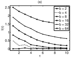
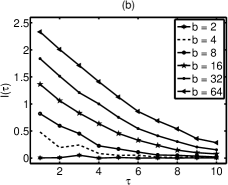
Figure 1: Average of ${\it I}(\tau)$ from the equidistant histogram-based estimator for lags $\tau=1,\ldots,10$ from $1000$ simulations of the Henon map for different number of bins (as in the legend) and for lengths $n=1024$ in (a) and $n=10^{7}$ in (b).

The simulation on the different systems showed that the equidistant estimator depends on $b$ and $n$, differently for small and large lags.

With the addition of noise, variations in the estimated mutual information in terms of $n$ and $b$ become smaller. However, this is expected as ${\it I}(\tau)$ decreases with the increase of noise level (see Fig.2).

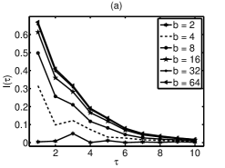
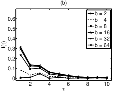
Figure 2: ${\it I}(\tau)$ from the equidistant estimator for lags $\tau=1,\ldots,10$ from one realization of the Henon map of length $n=10^{7}$, for noise level $20\%$ in (a) and $40\%$ in (b).

The inclusion of stronger noise component masks the deterministic structure and thus levels the estimate of mutual information towards zero. On the other hand, the benefit of noise in terms of stable estimation, is that ${\it I}(\tau)$ gets less dependent on $b$, e.g. in Fig.2 the estimate converges when $b>16$ for noise level at $20\%$ and $b>8$ for noise level at $40\%$.

For Mackey-Glass system, the ${\it I}(\tau)$ is computed for a range of lags that include the lag of first minimum of mutual information in order to assess also the accuracy of the estimator in detecting this particular lag. We observed that although ${\it I}(\tau)$ increases with $b$, the lag of the first minimum of mutual information does not vary with $b$. Moreover, the estimate of this lag is rather stable with $n$, as shown in Fig.3 for noise-free data and $\Delta=17$.

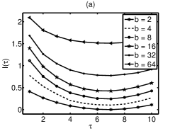
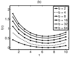
Figure 3: Average of ${\it I}(\tau)$ from the equidistant estimator for lags $\tau=1,\ldots,10$ from $1000$ realizations of the Mackey Glass system (sampling time 17) with $\Delta=17$ of length $n=1024$ in (a) and ${\it I}(\tau)$ from one realization of length $n=10^{6}$ in (b).

III.4 Equiprobable estimator

The EP estimator has the same form of dependence on $b$, $n$ and $\tau$ as the ED estimator. Moreover, the estimated ${\it I}(\tau)$ values from the two estimators may vary for small $n$ but converge with $n$, as shown for the noise-free data from the Ikeda system in Fig.4.

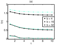
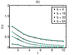
Figure 4: Average of ${\it I}(\tau)$ from the equidistant estimator (black lines) and the equiprobable estimator (gray lines, cyan in the color online) for lags $\tau=1,\ldots,10$ from $1000$ realizations of the Ikeda map for different number of bins (as in the legend), for lengths $n=256$ in (a) and $n=8192$ in (b).

Other works seem to agree with the result that estimators using a fixed partition heavily depend on the selection of $b$ Bonnlander and Weigend (1994); Cellucci et al. (2005); Trappenberg et al. (2006). Given that the chaotic systems have significant mutual information at least for very small lags and that the ED and EP estimators get close to zero for small number of bins, we conclude that a small $b$ is a good choice for these estimators only for independent time series. (We observed the same for linear stochastic systems in a different study.) To the contrary, for chaotic systems a refined partition explores in more detail the fine structure of the distribution (marginal and joint) and gives better estimate of the true mutual information. We would expect that in the limit of fine partition, where the expression of the discretized version of mutual information in (2) converges to the true mutual information in (1), ${\it I}(\tau)$ would converge as well, but this would require an infinite amount of data. Thus a good choice of bin width should balance a large $b$ with the limited size $n$ of the available data in order to maintain a good estimation of the probabilities in (2), in particular at regions with low data densities that may carry valuable information for the system dynamics. For a fixed $b$, the ED and EP estimators are rather stable with respect to $n$, i.e. they are consistent estimators of the mutual information as defined in (2) for the specific partition determined by $b$.

III.5 Adaptive histogram-based estimator

The AD estimator of Darbellay and Vajda is apparently independent of a parameter for the partitioning. However, it has a direct dependence on $n$, which determines the roughness of the partitioning in a somehow automatic way. In the abundance of data, the AD estimator reaches a very fine partition that satisfies the independence condition in each cell, so that the total number of cells is very large (analogously to a fixed-partition with a respectively large $b$). Thus the increase of $n$ implies a finer partition and explains the increase of ${\it I}(\tau)$ from the adaptive estimator with $n$, as shown for the Henon map in Fig.5a. Note that the dependence of AD on $n$ is not comparable to that of the fixed-bin estimators because it involves a change of partitioning with $n$. In this sense, AD is not consistent with respect to $n$. However, in the presence of noise, the effect of $n$ on the adaptive estimator decreases with the noise level (see Fig.5b).

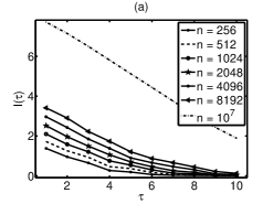
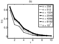
Figure 5: Average of ${\it I}(\tau)$ from the adaptive histogram-based estimator for lags $\tau=1,\ldots,10$ from $1000$ realizations of the Henon map for different lengths $n$ (as in the legend), for noise-free data in (a) and noisy data at $20\%$ noise level in (b).

AD is considered to be one of the most precise and efficient algorithms for estimating the mutual information that converges fast to the true mutual information, basically for certain distribution and Gaussian processes where this is analytically given Kraskov et al. (2004); Trappenberg et al. (2006). However, in the case of nonlinear systems the estimator does not seem to converge with $n$, unless the fine partition is limited by the presence of noise.

III.6 $k$-nearest neighbor estimator

The parameter of the number of nearest neighbors $k$ in this estimator determines the roughness of approximation of the density functions in (1), which corresponds to the roughness of the partitioning in (2). Thus for a fixed $n$, as ${\it I}(\tau)$ from fixed-bin estimators increase with $b$ (finer partition), the ${\it I}(\tau)$ from KNN increases when $k$ decreases, as shown in Fig.6a and b.

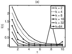
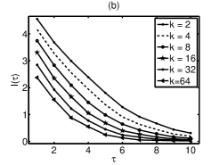
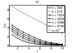
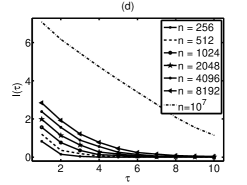
Figure 6: Average of ${\it I}(\tau)$ from the $k$-nearest neighbor estimator for lags $\tau=1,\ldots,10$ from $1000$ realizations of the Henon map. In (a) and (b) the results are displayed for different $k$ (as in the legend) and for $n=256$ and $n=8192$, respectively. In (c) and (d) the results are displayed for different $n$ (as in the legend) and for $k=2$ and $k=32$, respectively.

This dependence persists also for very large $n$, whereas for a small time series a large $k$ gives a poor estimation of the densities and consequently of ${\it I}(\tau)$ (see Fig.6a, particularly when $k=64$ and $n=256$).

We also observed that ${\it I}(\tau)$ increase with $n$ for a fixed $k$ (see Fig.6c and d). Assuming a fixed parameter ($k$ and $b$) the effect of $n$ on KNN is larger than on the fixed-bin estimators and similar to the effect of $n$ on the adaptive histogram-based estimator.

In agreement with the histogram-based estimators, KNN decreases with the noise level (see Fig.7).

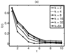
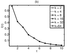
Figure 7: Average of ${\it I}(\tau)$ from the $k$-nearest neighbor estimator for lags $\tau=1,\ldots,10$ from $1000$ realizations of the Henon map with $20\%$ noise of length $n=1024$ in (a) and $I(\tau)$ from one realization of length $n=10^{7}$ in (b).

However in the presence of noise, the dependence of the KNN on $k$ is less than the dependence of the ED and EP on $b$ (e.g. for the case of Henon map with $n=10^{7}$ and $20\%$ noise level compare Fig.7b to Fig.2a). This results is in agreement with Nicolaou et al. Nicolaou and Nasuto (2005) that found independence of this estimator on $k$ for EEG data.

An upper limit for $k$ is set by $n$ whereas the lower limit $k=1$ corresponds to the finest partition we could get for a histogram-based estimator. Thus the restriction to small $k$ proposed by Kraskov et al. Kraskov et al. (2004) and used in other simulation studies Kreuz et al. (2007); Khan et al. (2007), corresponds to fine partitions. Thus for chaotic systems that require fine partitioning, a fair comparison of the KNN for these $k$ values to ED and EP would require a very large $b$. To this respect, this simulation comparison is restricted to comparable small $b$ (up to 64) due to computational limitations.

III.7 Kernel estimator

Among different kernel functions used in the literature for density estimation, and for mutual information estimation in particular, the common practice is to use the Gaussian kernel in conjunction with the ”Gaussian” bandwidth of Silverman Moon et al. (1995) or multiplies of it Harrold et al. (2001); Steuer et al. (2002); Khan et al. (2007). There are some other criteria for bandwidth selection that we have included in this study (see Table 1). Moreover, we test the KE estimator of mutual information also for a range of bandwidths as for the other estimators.

First we investigate the inter-dependence in the selection of $h_{1}$ and $h_{2}$ across the selected range of bandwidths. As shown in Fig.8 for the Henon map, selecting $h_{2}=\sqrt{2}h_{1}$ instead of $h_{2}=h_{1}$ simply decreases the value of $I(\tau)$, without alerting the form of the dependence of $I(\tau)$ on $\tau$ and this occurs independently of $n$.

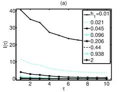
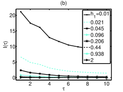
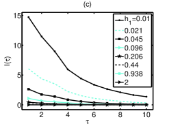
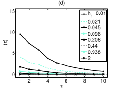
Figure 8: Average of ${\it I}(\tau)$ from the kernel estimator for lags $\tau=1,\ldots,10$ from $1000$ realizations of the Henon map for a range of different values of bandwidth $h_{1}$ (as in the legend). (a) $n=512$ and $h_{2}=h_{1}$, (b) $n=512$ and $h_{2}=\sqrt{2}h_{1}$, (c) $n=8192$ and $h_{2}=h_{1}$, (d) $n=8192$ and $h_{2}=\sqrt{2}h_{1}$

So, the roughness of the partitioning is determined by $h_{1}$, i.e. smaller $h_{1}$ implies finer partitions or small neighborhoods with respect to KNN. We note however that $\it{I}(\tau)$ from KEreaches very small values for as large $h_{1}$ as 2 and very large values for as small $h_{1}$ as $0.01$. Note that such extremely large values of ${\it I}(\tau)$ do not occur by any other estimator.

Regarding the 9 criteria selecting $h_{1}$ (and at cases $h_{2}$, see Table 1), the estimated bandwidths vary but within a small range (for $n=512$ in Fig. 9a they are bounded in [0.1,0.3] except C3 that always gives larger bandwidths where in this case is $h_{1}\simeq 0.64$).

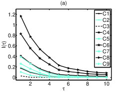
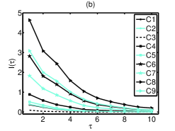
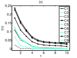
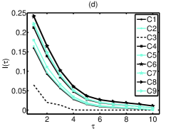
Figure 9: Average of ${\it I}(\tau)$ from the kernel estimator for lags $\tau=1,\ldots,10$ from $1000$ realizations of the Henon map from the nine bandwidth selection criteria for noise-free data and for $n=512$ in (a) and $n=8192$ in (b) and for $20\%$ noise level and $n=512$ in (c) and $n=8192$ in (d).

All criteria depend on $n$ in a similar way and estimate smaller bandwidths as $n$ increases giving larger ${\it I}(\tau)$ (see Fig. 9a and b). Thus a kernel estimator using a specific criterion turns out not to be consistent.

When noise is added to the time series ${\it I}(\tau)$ decreases and differences with respect to the partitioning parameters are smaller, as observed in the other estimators. This holds also when a specific bandwidth selection criterion is used, and in particular the estimated ${\it I}(\tau)$ is rather stable to the change of $n$ (see Fig. 9c and d).

In the estimation of mutual information with kernels, the range of bandwidths is usually not searched and a bandwidth is selected according to a criterion such as the ”Gaussian” bandwidth Steuer et al. (2002). However, our simulations have shown that KE estimator is strongly dependent on the bandwidth that defines the partition differently according to the sample size, and these findings are in agreement with other works Bonnlander and Weigend (1994); Jones et al. (1996).

III.8 Evaluation of estimators and their parameters

The results on the different estimators have shown a varying sensitivity of the estimator to its free parameter, where histogram-based estimators turned out to be the most sensitive. However, there seems to be a loose correspondence among the different free parameters $b$, $k$ and $h_{1},h_{2}$ depending also on the time series length. Thus the differences in the performance of the estimators can be explained to some degree by the coarseness of the partition as determined by its free parameter. The choice of $b$ for the histogram-based estimators determines the bin size of the partition. The analogue of the bin size for the $k$-nearest neighbors estimator is the size of neighborhoods and for the kernel estimator is the size of the efficient support for the kernel given by the bandwidth.

In order to check the correspondence of the estimator specific parameters, first we set a specific bin length $r$ for the partition given by $b$. For KNN the parameter $k$ is set to the average number of neighbors within each disc of diameter $r$. For KE we set $h_{2}=r/2$. In this way, we attempt to match the partition for each estimator. However, this selection scheme for the parameters does not result in similar estimated values of ${\it I}(\tau)$. For example, for a time series of the Henon map with length $n=512$ when $b=16$ the estimates of ${\it I}(\tau)$ seem to agree at some degree where as when $b=32$ they vary significantly, as shown in Fig.10.

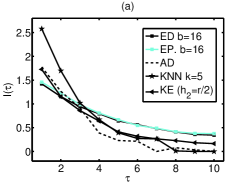
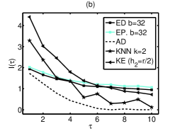
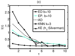
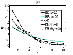
Figure 10: ${\it I}(\tau)$ from one realization of the Henon map of from all estimators, for parameters as in the legends for $n=512$ in (a), (b) and (c) and $n=1024$ in (d).

When the standard criteria for the selection of the parameters are considered, i.e. $b=\sqrt{n/5}$, $k=3$, and bandwidths $h_{1},h_{2}$ given by the Silverman’s criterion, the estimates of ${\it I}(\tau)$ vary even more (see Fig.10c). For a bit larger length as $n=1024$ we observed that if we choose a bit larger value of $b$ as $b=20$, we get similar estimated values of ${\it I}(\tau)$(see Fig.10d).

[to revise this according to the results on differen $n$ and for the other systems.] We concluded that the optimization of parameters is very crucial even more than the choice of the estimator, as we can see that no estimator exhibits consistency especially in the case of noise-free data.

It is also important to compare the computational cost of the estimators. The kernel estimator has the highest computational cost and the computation time for the histogram-based estimators is also prohibitive for very large values of $b$. The adaptive estimator has the advantage of being fast and parameter-free but tends to give larger ${\it I}(\tau)$ (compared to the other estimators) for small noise-free time series.

Most of the results of the different estimators are illustrated for the Henon map in order to facilitate comparisons, but qualitatively similar results are obtained from the simulations on the Ikeda map and the Mackey-Glass system.

IV Discussion

Mutual information estimators are not consistent for non-linear noise-free systems and the choice of parameters is crucial for all estimators. We cannot find an optimal parameter choice as there is no consistency. However with addition of noise in the systems, the choice of the parameters is not that crucial as there is convergence of the estimated ${\it I}(\tau)$ values and all estimators seem to be consistent especially for larger time series lengths. $k$-nearest neighbor estimates of ${\it I}(\tau)$ varies less with the free parameter ($k$) compared to the other estimators.

As a general conclusion we can say that all estimators depend on the parameter choice and therefore is crucial to optimize their parameter. Also consistency of estimators for linear systems is not indicative of the estimators behavior for nonlinear systems. Although consistency of estimators is claimed in many past works might be due to inclusion of only linear systems in their evaluation or presence of noise (e.g. real data).

However, this shows that the $k$-nearest neighbor estimator is computationally more effective when fine partitions are sought, due to the use of effective data structures in the search for neighbors.