Abundances and Isotope Ratios in the Magellanic Clouds: The Star Forming Environment of N 113

Abstract

With the goal of deriving the physical and chemical conditions of star forming regions in the Large Magellanic Cloud (LMC), a spectral line survey of the prominent star forming region N113 is presented. The observations cover parts of the frequency range from 85 GHz to 357 GHz and include 63 molecular transitions from a total of 16 species, among them spectra of rare isotopologues. Maps of selected molecular lines as well as the 1.2 mm continuum distribution are also presented. Molecular abundances in the core of the complex are consistent with a photon dominated region (PDR) in a nitrogen deficient environment. While CO shows optical depths of order $\tau$$\sim$10, ¹³CO is optically thin. The most prominent lines of CS, HCN, and HCO⁺ show signs of weak saturation ($\tau$$\sim$0.5). Densities range from 5$\times$10³ cm^-3 for CO to almost 10⁶ for CS, HCN, and a few other species, indicating that only the densest regions provide sufficient shielding even for some of the most common species. An ortho- to para-H₂CO ratio of $\sim$3 hints at H₂CO formation in a warm ($\mathrel{\mathchoice{\vbox{\offinterlineskip\halign{\hfil$\displaystyle#$\hfil\cr>\cr\sim\cr}}}{\vbox{\offinterlineskip\halign{\hfil$\textstyle#$\hfil\cr>\cr\sim\cr}}}{\vbox{\offinterlineskip\halign{\hfil$\scriptstyle#$\hfil\cr>\cr\sim\cr}}}{\vbox{\offinterlineskip\halign{\hfil$\scriptscriptstyle#$\hfil\cr>\cr\sim\cr}}}}$40 K) environment. Isotope ratios are ¹²C/¹³C $\sim$ 49$\pm$5, ¹⁶O/¹⁸O $\sim$ 2000$\pm$250, ¹⁸O/¹⁷O $\sim$ 1.7$\pm$0.2 and ³²S/³⁴S $\sim$ 15. Agreement with data from other star forming clouds shows that the gas is well mixed in the LMC. The isotope ratios do not only differ from those seen in the Galaxy. They also do not form a continuation of the trends observed with decreasing metallicity from the inner to the outer Galaxy. This implies that the outer Galaxy, even though showing an intermediate metallicity, is not providing a transition zone between the inner Galaxy and the metal poor environment of the Magellanic Clouds. A part of this discrepancy is likely caused by differences in the age of the stellar populations in the outer Galaxy and the LMC. While, however, this scenario readily explains measured carbon and oxygen isotope ratios, nitrogen and sulfur still lack a self-consistent interpretation.

1 Introduction

The Magellanic Clouds are two southern irregular galaxies that provide unique opportunities to study astrophysical processes (e.g., Westerlund 1990). Noteworthy are their extremely small distances ($\sim$50 and 60 kpc), low heavy element contents, low dust-to-gas mass ratios, high [O/C] and [O/N] elemental abundance ratios, high atomic-to-molecular hydrogen (H/H₂) ratios, and an intense ultraviolet (UV) and far-ultraviolet (FUV) radiation field. The Magellanic Clouds, which are much smaller than the Milky Way, are characterized by a lower degree of nuclear processing than the Galaxy. Right now, however, they are undergoing an episode of vigorous star formation.

In the past couple of decades there have been an enormous number of studies of the Magellanic Clouds (see, e.g., the IAU Symposia No. 108, 148 190, and 256). The first systematic molecular surveys, covering the central parts of the Magellanic Clouds in the CO $J$=1–0 line were those of Cohen et al. (1988) and Rubio et al. (1991) with angular resolutions of 8$\,.\!\!^{\prime}$8. More detailed CO surveys were carried out with the NANTEN telescope at 2$\,.\!\!^{\prime}$6 resolution (e.g., Yamaguchi et al. 2001; Mizuno et al. 2006). CO data with even higher resolution, obtained in the $J$=1–0 and 2–1 lines with 50^′′ and 25^′′ beamwidth, were taken with the SEST (Swedish-ESO Submillimeter Telescope). Several articles were published as part of the SEST Key-Program on CO in the Magellanic Clouds (e.g., Israel et al. 2003).

While these studies provide an overall view of the well shielded molecular medium in the Magellanic Clouds, multiline studies investigating the physical and chemical properties of the gas only exist for a very small number of targets in the vicinity of prominent HII regions. Following the pioneering study of Johansson et al. (1994) on N 159 in the LMC, Chin et al. (1997, 1998) and Heikkilä, et al. (1998, 1999) published molecular multi-line studies on star forming regions in the Magellanic Clouds. First detections of deuterated molecules outside the Galaxy were reported by Chin et al. (1996b) and Heikkilä, et al. (1997).

N 113, located in the central part of the LMC more than 2^∘ west of 30 Dor, is hosting the most intense H₂O maser of the Magellanic Clouds (Whiteoak & Gardner 1986; Lazendic et al. 2002; Oliveira et al. 2006). OH maser emission was also observed (Brooks & Whiteoak 1997). An IRAS (InfraRed Astronomy Satellite) point source, IRAS 0513–694, is associated with N 113. While Chin et al. (1996b, 1997) and Wong et al. (2006) collected single-dish and interferometric data from some $\lambda$3 mm transitions, a dedicated molecular multiline study of this star forming region covering the $\lambda$1–3 mm band is still missing. To improve our understanding of the interstellar medium (ISM) associated with massive star formation in an environment with low metallicity and to obtain a comprehensive view onto one of the most remarkable star forming regions of the LMC, we mapped the 1.2 mm continuum, obtained a spectral survey of the central region, and also mapped the cloud in several molecular lines.

2 Observations

2.1 1.2 mm continuum observations

In October 2002 and August 2003 the 15-m SEST Imaging Bolometer Array SIMBA was used to image the distribution of continuum emission at 250 GHz ($\lambda$1.2 mm) associated with N113. The 37-channel instrument was configured to map an area with dimensions of 400″ in azimuth and 392″ in elevation by means of 51 successive azimuth scans, at 80″/sec, with a separation of 8″ in elevation. Including overhead, a completed map took about six minutes. A total of 32 maps were obtained, 20 during the first observing period and 12 during the second.

At 250 GHz, the SEST beam had a full width to half maximum (FWHM) of $\sim$24″. Accurate pointing and focus of the antenna were maintained with periodic observations of point-source calibrators (mainly OA 129). Periodic ‘skydip’ observations provided estimates of the sky opacity. The derived zenith optical depths for both observing periods averaged about 0.14. Flux density calibration was provided by observations of Uranus, and were based on an adopted brightness temperature of 93 K for the planet.

The observations were processed using MOPSI, a software program developed and upgraded by R. Zylka (IRAM/Grenoble). Images were produced for each set of scans, and these were averaged to produce an image gridded in right ascension and declination. To reduce systematic baseline effects, the area containing the main source emission was defined by a polygon boundary, and this area was excluded from baselining corrections in a second averaging process. The algorithm PLANET enabled a flux density/beam scale to be derived from the Uranus observations.

2.2 Spectroscopic measurements

2.2.1 SEST 15-m observations

With the SEST, observations were carried out in January and September 1995, January and March 1996, January, March, July, and September 1997, July 1998, and July 1999. For the frequency ranges, single-sideband system temperatures on a main beam brightness temperature scale ($T_{\rm mb}$), beam widths and linear resolutions, see Table 1. 3 and 2 mm or 3 and 1.3 mm SIS receivers were employed simultaneously. For the SIS receiver used at 330–357 GHz, see also Mauersberger et al. (1996b).

The backend was an acousto-optical spectrometer (AOS) which was split into 2$\times$1000 contiguous channels for simultaneous $\lambda$$\sim$3 and 2 mm observations. At $\lambda\sim$1.3 and 0.85 mm, all 2000 channels were used to cover a similar velocity range. The channel separation of 43 kHz corresponds to 0.04–0.15 km s^-1 for the frequency interval 357–85 GHz.

All measurements were made with a circular rotating disk to enable the beam to be either reflected or to pass through to a mirror system behind it. The two light beams allowed us to observe in a dual beam switching mode with a switching frequency of 6 Hz (controlled by the rotational speed of the disk) and a beam throw of 11^′40^′′ in azimuth. Since rapid beam switching was used in conjunction with reference positions on both sides of the source, baselines are of good quality. Calibration was obtained with the chopper wheel method. Main beam efficiencies of 0.746, 0.683, 0.457 and 0.30 at 94, 115, 230, and 345 GHz, respectively, were derived from measurements of Jupiter (L. Knee, priv. comm.; see also Table 1). These values were interpolated and, if neccessary, also extrapolated to convert antenna ($T_{\rm A}^{*}$) to main beam brightness ($T_{\rm mb}$) temperature. The pointing accuracy, obtained from measurements of the nearby SiO maser source R Dor, was mostly better than 10^′′ (see also Sect. 3).

2.2.2 APEX 12-m observations

In October 2007, observations of the CO $J$=3–2 line were carried out with the double sideband APEX-2a facility receiver (Risacher et al. 2006). 145 positions were measured in a position switching mode with an on-source integration time of 40 sec and a beamwidth of $\sim$20″ (see Table 1). The beam efficiency was 0.73 and the forward hemisphere efficiency 0.97 (Güsten et al. 2006). Both units of a Fast Fourier Transform Spectrometer with 1 GHz bandwidth and 16384 channels each (Klein et al. 2006) were used to measure the CO transition. System temperatures on a $T_{\rm A}^{*}$ scale were 300–450 K.

3 Results

Figure 1 shows a 1.2 mm continuum map that is sensitive to the column density of the interstellar dust. Outside the core of N 113, which shows an elongation along an axis extending from the north-west to the south-east, we find protrusions toward the north and east, the latter only slighty surpassing the noise level. Figure 2 shows the corresponding distribution of integrated CO $J$=3–2 emisison. While the morphology appears to be similar, the eastern tongue is detected with higher significance. The dashed outer contour still represents a 6$\sigma$ level.

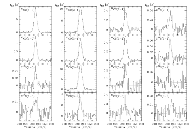
Figure 3: CO and CS spectra measured toward N113 ($\alpha=05^{\rm h}13^{\rm m}18.2^{\rm s}$, $\delta=-69^{\rm o}22^{\prime}35^{\prime\prime}$ (J2000)). The channel spacing for each spectrum is $\sim\,$0.9 km s^-1. Gaussian fits were performed for detected and tentatively detected lines, and resulting parameters are listed in Table 2 (same in Figs. 4–6).

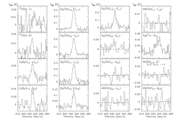
Figure 4: CS, C₃H₂, H₂CO, HDCO, N₂H⁺, NO and HNCO spectra measured toward N113. In the case of N₂H⁺, the frequency of the main hyperfine component (93.713809 GHz) is taken as reference. In Table 2, however, the expected average frequency for optically thin emission and Local Thermodynamical Equilibrium is displayed. For further details, see Fig. 3.

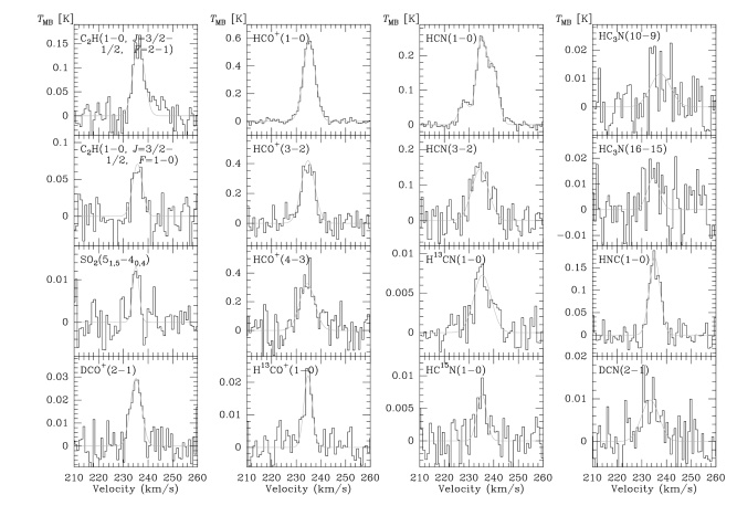
Figure 5: C₂H, SO₂, DCO⁺, HCO⁺, HCN, HC₃N, HNC, and DCN spectra measured toward N113. For details, see Fig. 3.

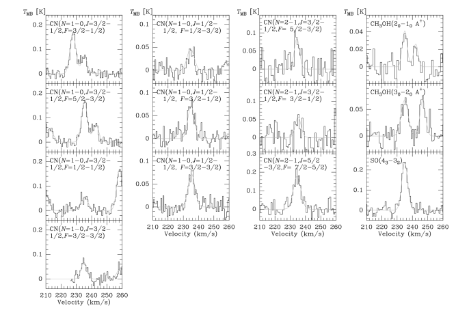
Figure 6: CN, CH₃OH, and SO spectra measured toward N113. The CH₃OH figures also show the 2_-1–1_-1 E and 3_-1–2_-1 E lines at slightly higher velocities than the 2₀–1₀ A⁺ and 3₀–2₀ A⁺ profiles, respectively. For further details, see Fig. 3.

Figures 3–6 display the spectra measured toward the peak of N 113. Agreement between the APEX and SEST CO $J$=3–2 spectra at the central position is reasonably good (peak line temperatures are 10.5 and 12 K on a $T_{\rm mb}$ scale, respectively). SEST line parameters are given in Table 2 and include 50 detected, 7 tentatively detected, and 6 undetected transitions. The ¹²C³⁴S $J$=5–4, ¹²C³³S 3–2, ¹³C³²S 2–1, and HC₃N 10–9 spectral features show deviations from a radial velocity of $\sim$235 km s^-1. These are, however, likely caused by noise, as the emission in the above transitions is significantly weaker than in the other listed lines of CS. The relatively high velocity of the N₂H⁺ 1–0 transition (Table 2) may be a consequence of the presence of seven hyperfine components. Deviations from the relative intensities expected in the case of Local Thermodynamic Equilibrium (LTE) could shift the line by $\sim$1–2 km s^-1. Alternatively, an exceptional drift in the velocity scale of the temperature sensitive backend cannot be excluded. Among the 16 molecules observed (this includes 28 “isotopologues”, i.e. species containing different isotopic substitutions), only two remain undetected, NO and HCNO. Both contain nitrogen.

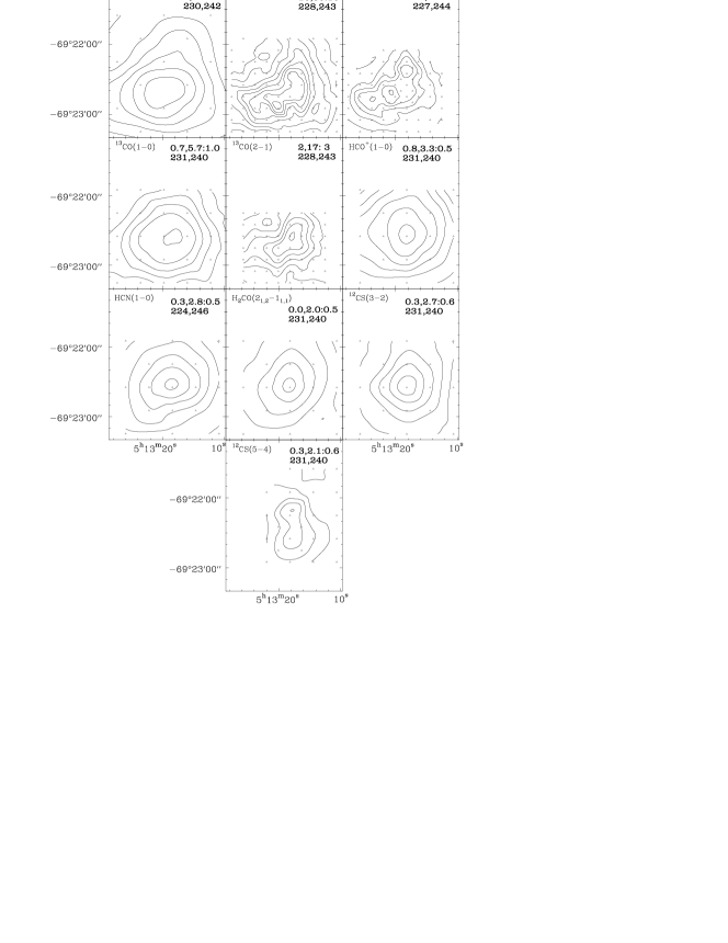
Figure 7: SEST CO, HCO⁺, HCN, H₂CO, and CS maps toward N113. The upper left corner of each panel indicates the molecular transition; the upper right corner gives the lowest contour, the highest contour, and the increment in K km s^-1 (upper line) and the velocity range in km s^-1 (lower line).

Also obtained were small maps in 10 molecular lines, including CO, ¹³CO, and the higher density tracers CS, HCN, HCO⁺, and H₂CO. Observed positions and contour plots are displayed in Fig. 7. The maps outline to a certain degree the extent of the molecular cloud. Since its size is, however, often comparable to the size of the beam of the telescope, a deconvolution of the beam was necessary. The results of this deconvolution are given in Table 3. Shown are the transition (Cols. 1 and 2), the beam width (Col. 3), the observed Full Width to Half Power (FWHP) source size in right ascension and declination (Cols. 4 and 5), the deconvolved extent in right ascension and declination (Cols. 6 and 7) and its geometric mean (Col. 8). In view of map spacing and possible pointing errors, resulting intrinsic source sizes are not acccurate. Thus for CO $J$=3–2 SEST (Fig. 7) and APEX (Fig. 2) data deconvolved source sizes are 40 and 60″, respectively. For HCN, the intrinsic size of the emitting region remains undetermined, while the half power extent of the $\lambda$1.2 mm continuum emission appears to be intermediate between those of CO $J$=1–0 and 2–1 and the average value derived from the molecular high density tracers (see Sect. 4.2 for adopted source sizes).

4 Discussion

N 113 is with N 159 one of the two strongest molecular line emitters of the Magellanic Clouds. Prior to a detailed analysis of our spectra, some general source properties should be mentioned. From the IRAS flux densities (5.7, 40.5, 268, and 415 Jy at 12.5, 25, 60, and 100$\mu$m, respectively) we obtain a total luminosity of $\sim$2$\times$10⁶ L_⊙ for N 113, extrapolating from 6 to 400$\mu$m and assuming a grain emissivity proportional to $\nu$ (see Wouterloot & Walmsley 1986). Wong et al. (2006) collected $\lambda$3 mm SEST, Mopra, and ATCA (Australia Telescope Compact Array) data of the radio continuum and prominent molecular species toward N 113. While the 3 mm continuum only reveals a flux density of $\sim$40 mJy from a 5–10″ sized source (presumably, there is missing flux), their SEST HCN and HCO⁺ spectra toward the cloud core are consistent with our data. In agreement with our measurements (Fig. 7, Table 3), their SEST and Mopra maps also show a source that is only slightly more extended than the telescope beam. The interferometric high resolution ATCA maps did not collect the entire flux but reveal a compact cloud core of size 8″$\times$5″, with HCO⁺ $J$=1–0 being presumably more extended than HCN $J$=1–0.

In the following we first discuss the $\lambda$1.2 mm continuum (Sect. 4.1) and then proceed to the analysis of spectral lines from individual molecular species (Sects. 4.2 and 4.3). Summaries of the observed properties with respect to H₂ densities (Sect. 4.4), molecular column densities (Sect. 4.5), and stellar nucleosynthesis (Sect. 4.6) follow.

4.1 The dust continuum

The 60 and 100$\mu$m IRAS fluxes and an emissivity proportional to $\nu$ yield a dust color temperature of $T_{\rm d(60/100)}$ = 42.5 K. With an integrated $\lambda$1.2 mm flux density of 1.6 Jy (see Fig. 1) and an emissivity proportional to $\nu^{2}$ we obtain a 100$\mu$m to 1.2 mm dust color temperature $T_{\rm d(100/1200)}$ = 21 K. The uncertainty in the 1.2 mm flux density of $\pm$20% causes an error in $T_{\rm dust}$ that does not surpass $\pm$2 K. Applying the equation given in Table 3 of Mauersberger et al. (1996a), we then obtain for dust temperatures between 20 to 45 K a total gas mass of $M_{\rm N113}$ = (6.7 – 3.0)$\times$10⁵ M_⊙. This assumes a dust to gas mass ratio of 500, which is a factor of four higher than in the solar neighborhood (Bolatto et al. 2000). For the 24^′′ sized central area (420 mJy), the column density becomes (1.0 – 0.5)$\times$10²³ cm^-2 for the range of plausible dust temperatures (see Sect. 4.2.1 for the corresponding estimate from CO). The total mass estimated by us is a little larger than that given by Wong et al. (2006) who favored $M_{\rm N113}$$\sim$10⁵ M_⊙.

4.2 Molecules with LVG modelling

With a Large Velocity Gradient (LVG) model (e.g., Sobolev 1960; Castor 1970; Scoville & Solomon 1974) and choosing a spherically symmetric cloud geometry, the H₂ density and the column density of a given species can be estimated. As input this requires some knowledge of the kinetic temperature as well as line intensities from a sufficient number of transitions of a given molecule. The choice of a particular cloud geometry can affect resulting densities by up to half an order of magnitude, but only if the lines are optically thick. Applying a plane-parallel instead of a spherical cloud geometry can result in particle densities which are lower by up to this amount.

We correct for beam dilution by calculating $T^{\prime}_{\rm mb}$ = $T_{\rm mb}$/$\eta_{\rm bf}$ with $\eta_{\rm bf}$ = $\theta^{2}_{\rm s}$/($\theta^{2}_{\rm s}$+$\theta^{2}_{\rm b}$). $\theta_{\rm b}$ and $\theta_{\rm s}$ denote beam and source size, respectively (see also Wang et al. 2004). With the exception of a few CO lines (see Sect. 3) a source size of 40^′′ was assumed, which is consistent with the extent of the 1.2 mm continuum emission (Sect. 3, Fig. 1, and Table 3) and with the average of the (individually uncertain) molecular cloud size estimates of Table 3. Table 4 shows line temperatures prior and after correction for beam dilution.

The results of the model calculations that are based on the corrected line temperatures are shown in Figs. 8–13. Displayed are line intensities and peak line intensity ratios as a function of H₂ density and molecular column density.

In the following, LVG simulations are discussed for the most important molecular species. Calculations were made for kinetic temperatures of 20, 50, and 100 K (see e.g., Mangum & Wootten 1993, Chin et al. 1996b, and Heikkilä, et al. 1999 for a justification of the chosen temperature range).

4.2.1 CO

All of the eight lines of carbon monoxide (CO) shown in the left panels of Fig. 1 have been clearly detected. The lineshapes are compatible. While the ¹²C¹⁷O (hereafter C¹⁷O) $J$=1–0 line is broader than all other measured CO transitions, this is not an effect caused by a relatively low signal-to-noise level. Hyperfine splitting, leading to two blended main spectral features separated by a few km s^-1 (see Lovas & Krupenie 1974; Wouterloot et al. 2005), is broadening the line. A comparison of the ¹²C¹⁸O (hereafter C¹⁸O) and C¹⁷O $J$=1–0 lines results in an intensity ratio of 1.7$\pm$0.2 which is extremely low compared with galactic values measured by Penzias (1981) and Wouterloot et al. (2005). The line intensity ratio agrees, however, with the average ratio of 1.6$\pm$0.3 determined by Heikkilä et al. (1999) from the $J$=2–1 lines for a number of prominent Hii regions of the LMC. As a consequence it is reasonable to assume that C¹⁸O and C¹⁷O are optically thin and that potential differences in shielding (Heikkilä et al. 1999) are minimal (see Sect. 4.6).

Because of optical depth effects, an interpretation of the ¹²C¹⁶O (hereafter CO) and ¹³C¹⁶O (hereafter ¹³CO) spectra is less straightforward. With a ¹²C/¹³C isotope ratio of 49$\pm$5 (Sect. 4.2.3) and ¹²CO/¹³CO line intensity ratios of 7.1, 4.8 and 3.5 for the $J$=1–0, 2–1 and 3–2 transitions, respectively (see Tables 2 and 5), CO opacities must be of order $\tau$ $\sim$ 7, 10, and 14. These are consistent with opacities of typical galactic clouds (e.g. Larson 1981), but are much larger than $\tau$$\sim$1, which was proposed by Heikkilä et al. (1999) for the CO $J$=1–0 transition in other star forming regions of the LMC. For our estimate we have assumed that CO and ¹³CO excitation temperatures are similar and that fractionation (Watson et al. 1976) and isotope selective photodissociation (Bally & Langer 1982) are either not important or are balancing each other. For the Galaxy, prominent molecular clouds do not show strong differences in the relative abundances of ¹²C and ¹³C bearing isotopologues (for CO, CN, and H₂CO, see Milam et al. 2005). For the LMC this is less clear (e.g., Heikkilä et al. 1999). In any case, the measured CO/¹³CO line intensity ratios are large enough to ensure that ¹³CO is optically thin. Larger opacities resulting in the observed smaller ¹²C/¹³C line intensity ratios in the higher–$J$ rotational CO transitions are expected because of the higher statistical weights of the molecular states involved.

While ¹⁸O/¹⁷O and ¹²C/¹³C isotope ratios have previously been determined in several star forming regions of the LMC and while the gas appears to be well mixed, showing similar ratios in different sources (see Heikkilä et al. 1998 for the oxygen ratio), the higher and thus more elusive ¹⁶O/¹⁸O isotope ratio was so far only determined in N 159W (Heikkilä et al. 1999, their Table 16). With the ¹²C/¹³C isotope ratio directly obtained from the relative strengths of the HCN $J$=1–0 hyperfine components and the line intensity ratio of its ¹²C and ¹³C bearing species (Sect. 4.2.3 and Chin et al. 1999), a more accurate estimate is possible for N 113. If ¹³CO $J$=1–0 is optically thin as indicated above, the ¹⁶O/¹⁸O ratio is determined by multiplying the ¹³CO/C¹⁸O $J$=1–0 line intensity ratio by 49$\pm$5, which is the ¹²C/¹³C isotope ratio deduced from HCN (Sect. 4.2.3). We obtain ¹⁶O/¹⁸O = 2000$\pm$250. This result is in good agreement with the value given in Table 16 of Heikkilä et al. (1999) for N 159W, suggesting that the ratio, like that of ¹⁸O/¹⁷O, may not vary strongly from source to source. The ¹⁶O/¹⁸O value is four to ten times larger than corresponding ratios determined in the interstellar medium of spiral galaxies (e.g., Henkel & Mauersberger 1993). It yields a double isotope abundance ratio of ¹³CO/C¹⁸O $\sim$ 40, also consistent with the value proposed by Heikkilä et al. (1998) for N 159W. For ¹⁶O/¹⁷O, we obtain 3400$\pm$600.

With ¹²CO opacities of order 10, a carbon isotope ratio of $\sim$50, and the ¹⁶O/¹⁸O ratio determined above, ¹³CO should be optically thin not only in the $J$=1–0, but also in the 2–1 and 3–2 transitions. Multiplying the ¹³CO column density derived from LVG modeling by 50, taking collision rates with H₂ from Flower (2001), and assuming an ortho-to-para H₂ abundance ratio of 3:1 allows us to determine the total CO column density. With the LVG code we obtain $N$(CO)$\sim$6.5$\times$10¹⁷ cm^-2 and $n$(H${}_{2})$ $\sim$ 5$\times$10³ cm^-3. For a graphic display of the results that neither strongly depend on the choice of the collision rates nor on the ortho-to-para H₂ abundance ratio, see Fig. 7. The resulting values hold approximately for kinetic temperatures between 20 and 100 K.

Applying the mass estimate given by MacLaren et al. (1988) for a virialized cloud with an 1/$r$ density gradient, we find for a cloud size of $R$=5.5 pc (23″, Table 1; this is within the range of beam radii listed in Table 3) and a linewidth of 5 km s^-1, $N$(H₂) $\sim$ 1.7$\times$10²² cm^-2, $N$(CO)/$N$(H₂) $\sim$ 4$\times$10^-5, and $<$$n$(H₂)$>$$\sim$500 cm^-3. The CO/H₂ abundance ratio is about half that characterizing galactic clouds (e.g., Frerking et al. 1982). The conversion factor between H₂ column density and CO $J$=1–0 integrated intensity becomes with $I_{\rm CO~{}1-0}$ $\sim$ 50 K km s^-1 (Table 2) $X$ = $N$(H₂)/$I_{\rm CO~{}1-0}$ $\sim$ 3.4$\times$10²⁰ cm^-2 (K km s^-1)^-1. This is almost twice the value for the galactic disk (e.g., Mauersberger et al. 1996a, their Appendix A.1) and the value reported by Chin et al. (1997) on the basis of a small number of CO lines observed toward N 113. Since uncertainties amount to at least a factor of two, our value is still consistent with approximately galactic values on small spatial scales, as already suggested by Rubio et al. (1993) and Chin et al. (1997) for the Magellanic Clouds. The column density derived for a virialized cloud is smaller than that obtained from the dust continuum in Sect. 4.1. This may in part be caused by the different beams considered. If most of the dust emission would arise from the compact core seen by Wong et al. (2006), we had to multiply the $N$(H₂) = (5–10)$\times$10²² cm^-2 from the dust emission by (24″/45″)², yielding column densities of (1.4–2.8)$\times$10²² cm^-2. This agrees well with the virial estimate from the CO data.

4.2.2 CS

Ten lines of carbon monosulfide (CS) were observed. The results are shown in the right two panels of Fig. 3 and in the left panel of Fig. 4. While the three lower–$J$ lines of the main isotopic species, ¹²C³²S (hereafter CS), are clearly seen, the $J$=7–6 line is only tentatively detected. The rare isotopologue ¹²C³⁴S (hereafter C³⁴S) was detected in two and tentatively also in a third transition, while weak features are also seen at the frequencies of the $J$=2–1 and 3–2 lines of ¹³C³²S (hereafter ¹³CS) and of the $J$=3–2 line of ¹²C³³S (hereafter C³³S).

Are the lines of the main CS species optically thick, like those of CO? The $J$=3–2 transition, which is strongest, measured in four isotopologues, provides useful hints. For the CS/¹³CS $J$=3–2 line intensity ratio we obtain 37$\pm$5, which is a little less than the ¹²C/¹³C isotope ratio of $\sim$50 (Sect. 4.2.3). This implies that optical depths are not large, minimizing effects of isotope selective photodissociation. Deviations in the abundance ratio between the ¹²C and ¹³C bearing species of CS and HCN should also be small (Langer et al. 1984). Therefore neglecting these two effects, we obtain an optical depth $\tau$ $\sim$ 0.65 for the $J$=3-2 line of the main species, if CS and ¹³CS excitation temperatures are similar. For CS/C³⁴S $J$=3–2, the line intensity ratio is 11.3$\pm$1.1. This is about a factor of two lower than the abundance ratio measured towards N 159W (Heikkilä et al. 1999; their Table 16), again suggesting a moderate degree of saturation in the CS $J$=3–2 line. With $\tau$(CS 3–2)$\sim$0.65 as derived above, the ³²S/³⁴S sulfur isotope ratio becomes $\sim$15, slightly lower than values in the Galaxy (Chin et al. 1996a) and in N159W. If the tentatively detected C³³S $J$=3–2 line is really almost as strong as the ¹³CS $J$=3–2 line, this would imply ³²S/³³S $<$ 100. This value is smaller than the ratio of 120–150 found in the solar system, the local interstellar medium, and the late-type carbon star IRC+10216 (Mauersberger et al. 2004).

Because C³⁴S is certainly optically thin and exhibits stronger lines than the other rare CS species, it is the isotopologue of choice to simulate CS excitation and to determine CS column density and H₂ density. LVG calculations (collision rates from Turner et al. 1992) yield, multiplying the C³⁴S column by a factor of 15, $N$(CS) $\sim$ 2.5$\times$10¹³ cm^-2 and $n$(H₂) $\sim$ 10⁶ cm^-3 for kinetic temperatures between 20 and 100 K. With an H₂ density several orders of magnitude higher than that determined for CO, CS must trace a different kind of molecular gas.

4.2.3 HCN, HCO⁺ and HNC

HCN is detected in the $J$=1–0 and 3–2 transitions (Fig. 5) together with the rare isotopologues H¹³CN and HC¹⁵N, which were observed in the $J$=1–0 line, and DCN, which was measured in the $J$=2–1 line. For earlier discussions of isotope ratios, see Chin et al. (1996b, 1999). Here we emphasize that the HCN $J$=1–0 line is sufficiently narrow to show its hyperfine (HF) structure, i.e. three components with relative intensities of 5:3:1 in the optically thin limit under conditions of Local Thermodynamical Equilibrium (LTE). The ratios actually observed are 3.64:2.34:1 (errors are of order 10%), indicating a moderate degree of saturation in its stronger HF components. Comparing the intensity ratio between the weakest HF component ($\tau$$\sim$0.12, see Table 2 of Chin et al. 1999) and the H¹³CN line and multiplying this by the factor (5+3+1)=9 yields a ¹²C/¹³C isotope ratio of 49$\pm$5. This is presumably the most accurate carbon isotope ratio determined for the LMC because we were able to derive the ratio from optically thin lines (see, e.g., Johansson et al. 1994; Chin et al. 1996b; Heikkilä et al. 1999 for consistent but less accurate determinations in other star forming regions of the LMC). According to Langer et al. (1984), the ratio from HCN may be somewhat higher than the overall carbon isotope ratio, but in the Galaxy, such differences are found to be negligible (Milam et al. 2005). The ratio is thus used throughout the article. For details on ¹⁴N/¹⁵N and D/H, see Chin et al. (1996b, 1999).

Application of an LVG code (Fig. 10; collision rates from Schöier et al. 2005) yields H₂ densities of 8$\times$10⁵, 3$\times$10⁵, and 1.6$\times$10⁵ cm^-3 for kinetic temperatures of 20, 50, and 100 K. The column density is $N$(HCN) $\sim$ 6.3$\times$10¹² cm^-2.

HCO⁺ was detected in a total of five lines, in the $J$=1–0, 3–2 and 4–3 transitions of the main species, the $J$=1–0 transition of H¹³CO⁺ and the $J$=2–1 transition of DCO⁺ (first and second panel of Fig. 5). For the $J$=1–0 HCO⁺/H¹³CO⁺ line intensity ratio, we find 39$\pm$5, again suggesting a moderate optical depth of order 0.5 as in the case of the CS $J$=3–2 and HCN $J$=1–0 lines. LVG calculations (Fig. 11) indicate H₂ densities of 6$\times$10⁵, 2.5$\times$10⁵, and 1.6$\times$10⁵ cm^-3 and a column density of order 4$\times$10¹² cm^-2. Note that for $T_{\rm kin}$ = 20 K, the $J$=4–3/$J$=3–2 line intensity ratio cannot be reproduced, possibly suggesting that the kinetic temperature of the gas is higher in this star forming region. This induces a high uncertainty in the density estimate for this low kinetic temperature.

Because a rare HNC isotopologue has not been observed, the optical depth of its $J$=1–0 lines remains undetermined. Nevertheless, because the line is weaker than those of HCN and HCO⁺, the assumption of optically thin emission appears to be reasonable. Physical parameters of HCN and HNC are quite similar but chemical properties differ strongly (e.g., Schilke et al. 1992; Aalto et al. 2002). In spite of this assuming similar spatial distributions and excitation conditions, we tentatively obtain a total molecular column density of $N$(HNC) $\sim$ 2.5$\times$10¹² cm^-2.

4.2.4 H₂CO

At least five lines of formaldehyde (H₂CO) are seen (second and third panels of Fig. 4). Three belong with $K_{\rm a}$=1 to the ortho-species (the hydrogen atoms have parallel spin), two to the para-species ($K_{\rm a}$=0, antiparallel spin). A sixth line, also from para-H₂CO ($K_{\rm a}$ = 2) may have been tentatively detected and may serve as a tracer of kinetic temperature in future studies (Mühle et al. 2007). The rare isotopologue HDCO was searched for in two transitions but remains undetected. Our LVG calculations are based on collision rates of Green (1991) with He that were scaled upwards by a factor of 1.37 to approximate collisions with H₂. Results are presented in Fig. 11. Including 41 para- and 40 ortho-H₂CO levels with molecular states up to 300 cm^-1 above the ground state, the results are consistent with optically thin emission. The column density of ortho-H₂CO is about three times that of para-H₂CO. This result is independent of the assumed kinetic temperature (20 K$\leq$$T_{\rm kin}$$\leq$100 K; Fig. 11). Since the lines show signal-to-noise ratios of order 10, 1$\sigma$ errors are small and ortho-to-para abundance ratios below 2.5 or above 3.5 can be excluded. The ratio agrees with that expected in the case of formaldehyde formation in a warm ($T_{\rm kin}$$\mathrel{\mathchoice{\vbox{\offinterlineskip\halign{\hfil$\displaystyle#$\hfil\cr>\cr\sim\cr}}}{\vbox{\offinterlineskip\halign{\hfil$\textstyle#$\hfil\cr>\cr\sim\cr}}}{\vbox{\offinterlineskip\halign{\hfil$\scriptstyle#$\hfil\cr>\cr\sim\cr}}}{\vbox{\offinterlineskip\halign{\hfil$\scriptscriptstyle#$\hfil\cr>\cr\sim\cr}}}}$40 K) environment (e.g., Kahane et al. 1984; Dickens & Irvine 1999) and is not far off the value of 2.6, determined by Heikkilä et al. (1999) for N 159W. Densities vary between 10⁵ and 10⁶ cm^-3 but are, for a given kinetic temperature, within the uncertainties the same for ortho- and para-H₂CO. This and similar linewidths (see Table 2) suggest that both formaldehyde species reside in the same volume.

While our LVG model results seem to agree with optically thin emission, we do not have detections of rare isotopic species to prove this. HDCO is weaker than the main species by a factor of $\mathrel{\mathchoice{\vbox{\offinterlineskip\halign{\hfil$\displaystyle#$\hfil\cr>\cr\sim\cr}}}{\vbox{\offinterlineskip\halign{\hfil$\textstyle#$\hfil\cr>\cr\sim\cr}}}{\vbox{\offinterlineskip\halign{\hfil$\scriptstyle#$\hfil\cr>\cr\sim\cr}}}{\vbox{\offinterlineskip\halign{\hfil$\scriptscriptstyle#$\hfil\cr>\cr\sim\cr}}}}$30 (3$\sigma$). This is below the level found in the cool environment of some low-mass protostellar cores (e.g., Roberts et al. 2002; Parise et al. 2006) but does not provide significant constraints, neither to the optical depths of the main species nor to the cosmic D/H ratio (see e.g., Chin et al. 1996b; Heikkilä et al. 1997; Gerin & Roueff 1999 for details). With the lines assumed to be optically thin, column densities become $N$(para-H₂CO) $\sim$ 4$\times$10¹² cm^-2 and $N$(ortho-H₂CO) $\sim$ 1.2$\times$10¹³ cm^-2. These column densities do not strongly depend on the assumed kinetic temperature.

4.2.5 CH₃OH

Two $J$=2–1 and another two 3–2 lines of methanol (CH₃OH) were detected (last panel of Fig. 6). This is the first time that the rotational multiplets of methanol have been resolved in an extragalactic source (cf. Henkel et al. 1987; Heikkilä et al. 1999). At kinetic temperatures of $T_{\rm kin}$ = 50 and 100 K, the measured profiles lead to $N$(CH₃OH) $\sim$ 1.0$\times$10¹³ cm^-2 and $n_{\rm H_{2}}$ $\sim$ 3.2$\times$10⁴ cm^-3 assuming optically thin emission. At $T_{\rm kin}$ = 20 K, the density is poorly determined and may become $>$10⁵ cm^-3, while the column density is not significantly changed.

4.2.6 C₃H₂

Both detected lines of cyclic C₃H₂ (hereafter c-C₃H₂) belong to the ortho-species. Using an LVG code with collision rates from Chandra & Kegel (2000), we obtain densities of $n$(H₂) = 3$\times$10⁴ and 9$\times$10⁴ cm^-2 for $T_{\rm kin}$ = 100 and 25 K, respectively. The 1$\sigma$ uncertainty in the deconvolved line ratio, 0.39$\pm$0.08 (see Tables 2 and 4), which accounts for errors in the Gaussian fits, yields 1$\sigma$ deviations in density by a factor of 2. The column density becomes $N$(c-C₃H₂) $\sim$ 3$\times$10¹² cm^-2.

4.3 Other molecular species

4.3.1 CN

CN shows complex spectra. Each CN rotational state with $N$$>$0 is split into a doublet by spin-rotation interaction. Because of the spin of the nitrogen nucleus, each of these components is further split into a triplet of hyperfine states. Calculated frequencies and relative intensities are given by Skatrud et al. (1983).

CN was detected in a total of 10 lines, seven belonging to the 1–0 and three to the 2–1 transition. Relative intensities of the detected $N$=1–0 features agree within 20% with the LTE predictions. When comparing its measured relative intensity with the corresponding LTE value, the strongest line ($J$=3/2–1/2, $F$=5/2–3/2; weight: $\sim$33%) is weaker than expected by almost 20%. For the two lines with the second largest LTE weights ($\sim$12%), such a discrepancy is not apparent. We conclude that all CN $N$=1–0 features are not highly saturated, with the strongest feature having an optical depth of $\tau$$\mathrel{\mathchoice{\vbox{\offinterlineskip\halign{\hfil$\displaystyle#$\hfil\cr<\cr\sim\cr}}}{\vbox{\offinterlineskip\halign{\hfil$\textstyle#$\hfil\cr<\cr\sim\cr}}}{\vbox{\offinterlineskip\halign{\hfil$\scriptstyle#$\hfil\cr<\cr\sim\cr}}}{\vbox{\offinterlineskip\halign{\hfil$\scriptscriptstyle#$\hfil\cr<\cr\sim\cr}}}}$0.5.

The three $N$=2–1 observed transitions are also not providing evidence for high opacities. Here the line with intermediate intensity ($J$=3/2–1/2, $F$=5/2–3/2) is much weaker than expected. LTE ratios are 26.7:16.7:6.1, which should be compared with observed ratios of 31.5:10.6:7.4 (errors are of order 10–15%).

In the optically thin limit, the CN excitation temperature can be obtained from the ratio between the sum of the $N$=2–1 and 1–0 intensities using

$$R_{21}=4\times\ {\rm e}^{-x}\times\ \frac{1-{\rm e}^{-2x}}{1-{\rm e}^{-x}}\times\ \frac{({\rm e}^{2x}-1)^{-1}-({\rm e}^{2y}-1)^{-1}}{({\rm e}^{x}-1)^{-1}-({\rm e}^{y}-1)^{-1}},$$

with $x$ = h$\nu_{10}$/k$T_{\rm ex}$, $y$ = h$\nu_{10}$/(k $\times$ 2.73) and $\nu_{10}$ = 113.386 GHz (see Wang et al. 2004). While the integrated intensity of the $N$=1–0 transition is well determined (only two components representing together $\sim$2.5% of the total LTE intensity are not observed), the three measured $N$=2–1 features only provide $\sim$50% of the total intensity under LTE conditions. Thus the total $N$=2–1 intensity in $R_{21}$ is less well determined and, in view of potential deviations from LTE conditions, an error cannot be derived. Ignoring these uncertainties and accounting for the LTE intensities of the unobserved features, we obtain a line intensity ratio of 1.20. Correcting for the different beam sizes at 3 and 1.3 mm yields $R_{21}$ = 0.69 and $T_{\rm ex}$ = 5.6 K. This value is small, indicating subthermal excitation (see e.g., Fuente et al. 1995). The column density becomes $N$(CN) $\sim$ 3.5$\times$10¹³ cm^-2.

4.3.2 Other molecules

The remaining molecular species are seen in too few transitions and do not provide enough information for a reliable estimate of density and excitation. Assuming, however, that the lines are optically thin (a realistic assumption, see Sects. 4.2.2, 4.2.3, and 4.3.1) and realizing that the column densities are almost independent of the chosen kinetic temperature, column densities can still be estimated in some cases. This involves an educated guess of the density.

We detected strong SO emission in the 4₃–3₂ transition (Fig. 6). The column density (Table 5) was calculated with an LVG code (70 levels up to 580 K above the ground state; collsion rates from Green 1994) for $T_{\rm kin}$ = 50 K and $n$(H₂) = 5$\times$10⁴ and 5$\times$10⁵ cm^-3. The resulting column density becomes 1.5${}^{+1.5}_{-0.8}$$\times$10¹³ cm^-2.

Having observed two of the hyperfine components of the $N$=1–0 transition of C₂H, we find that their line intensity ratio, 2.4$\pm$0.4, is consistent with 2.0, the expected value for optically thin emission under LTE conditions. C₂H is present in UV irradiated molecular clouds as well as in well shielded cores (e.g., Pety et al. 2005; Beuther et al. 2008). Only having detected the $N$=1–0 transition, and with no LVG code at hand, a reliable column density could not be estimated (with the assumptions used by Wang et al (2004) for NGC 4945, the source averaged 5$\sigma$ upper limit would become 7$\times$10¹⁴ cm^-2).

N₂H⁺ was detected in the $J$=1–0 line (Fig. 4). Individual hyperfine components are, unlike those of HCN $J$=1–0, blended. For the column density (Table 5) an LVG code was used with 31 levels up to 2100 K above the ground state (collision rates from Schöier et al. 2005). With the parameters also used for SO, a column density of 7${}^{+1}_{-1}$$\times$10¹¹ cm^-3 was calculated.

For SO₂, detected in the 5_1,6–4_0,4 line, we used RADEX, an LVG code also calculating the radiative transfer for a homogeneous, isothermal sphere with high velocity gradient (van der Tak et al. 2007). The column density becomes 5${}^{+1}_{-1}$$\times$10¹² cm^-2.

HC₃N was tentatively detected in the $J$=10–9 and 16–15 transitions (Fig. 5). An LVG fit to the deconvolved brightness temperatures (22 levels up to 92 K above the ground state; collision rates from Green & Chapman 1978) yields for the determined upper limits and $T_{\rm kin}$ = 50 and 100 K densities of $n$(H₂) $\sim$ 3$\times$10⁵ cm^-3 and 1.5$\times$10⁵ cm^-3, respectively. $N$(HC₃N) $\mathrel{\mathchoice{\vbox{\offinterlineskip\halign{\hfil$\displaystyle#$\hfil\cr<\cr\sim\cr}}}{\vbox{\offinterlineskip\halign{\hfil$\textstyle#$\hfil\cr<\cr\sim\cr}}}{\vbox{\offinterlineskip\halign{\hfil$\scriptstyle#$\hfil\cr<\cr\sim\cr}}}{\vbox{\offinterlineskip\halign{\hfil$\scriptscriptstyle#$\hfil\cr<\cr\sim\cr}}}}$ 6$\times$10¹¹ cm^-2 (Table 5). A kinetic temperature of 20 K is too small to fit the two tentatively detected lines.

Adopting the excitation conditions assumed by Martín et al. (2006) for NGC 253, NO and HNCO source averaged 5$\sigma$ upper limits to the column density would become 6.5$\times$10¹⁴ cm^-2 and 2.6$\times$10¹³ cm^-2, respectively.

4.4 Densities and chemical implications

The determination of spatial densities depends to a certain degree on the assumed kinetic temperature. Nevertheless, Table 5 clearly shows that the molecular species analyzed in some detail emit from regions that are characterized by three different density regimes. CO traces, not unexpectedly, the lowest density component, C₃H₂ and CH₃OH originate from gas with intermediate density. All the other molecules detected in more than one line trace the high density component that can only occupy a small volume because it is three orders of magnitude denser than the $<$$n$(H₂)$>$ value derived for the inner 45″ of the cloud (Sect. 4.2.1).

CO, the studied species with by far the highest column density, has a natural advantage with respect to self-shielding in a hostile interstellar environment like that of the LMC (see Sect. 1). Furthermore, a small dipole moment leads to a particularly low “critical density”. Therefore collisional excitation to $T_{\rm ex}$ values well above the level of the cosmic microwave background is reached at comparatively low H₂ densities.

Cyclic C₃H₂ is a well known tracer of diffuse gas (e.g., Thaddeus et al. 1985; Cox et al. 1988) so that a lower density than for other species with a similarly high dipole moment is consistent with measurements of galactic clouds. However, such a similarity is not self-evident. UV photons that are abundant in the LMC (e.g., Israel et al. 1996) might destroy all c-C₃H₂ except in the densest regions. That this is not the case is an important finding.

Quasi-thermal methanol (CH₃OH) has been observed to be sandwiched between shocked regions, seen in vibrationally excited H₂, and CS, tracing the dense ambient medium (Liechti & Walmsley 1997; see also Table 5). Fractional methanol abundances can vary over several orders of magnitude (e.g., Kalenskii et al. 1997) and are sometimes drastically enhanced by grain mantle evaporation so that we may see emission arising preferentially from the outer, less dense, highly UV irradiated edges of the molecular complex.

CS, HCN, HCO⁺, and H₂CO trace the dense medium of N 113, but we should note that the CS, HCN, and HCO⁺ $J$ = 1-0 lines are slighty too strong for an optimal LVG fit. This suggests that some of their emission is also arising from the component with intermediate density. The $J$=1–0 line of para-H₂CO is not part of the 3 mm band and was therefore not observed. In galactic clouds HCO⁺ often arises from lower density gas than HCN (e.g., Baan et al. 2008). Toward N 113, we do not see this effect, which may imply that HCN and HCO⁺ are efficiently destroyed by photodissociation in the lower density parts of the cloud. There is some evidence that H₂CO may be related to photon dominated regions, i.e. to the lower density edges of molecular clouds that are irradiated by UV-photons. Toward M 82, another small galaxy with an intense UV field, Weiß et al. (2001) observed NH₃ and found that its emission must arise from relatively cool cloud cores that show a temperature similar to the overall dust radiation ($T_{\rm kin}$ $\sim$ 50 K). H₂CO, however, was found to trace a much warmer gas component, with $T_{\rm kin}$ $\sim$ 200 K and a surprisingly low density, $n$(H₂) $\sim$ 7$\times$10³ cm^-3 (Mühle et al. 2007). In M 82, H₂CO may be related to evaporated dust grain mantles (e.g., Ceccarelli et al. 2001), but apparently this scenario does not hold for N 113.

Overall, the densities obtained for CO and the higher density tracers are within the range estimated by Heikkilä et al. (1999) for a number of other star forming clouds in the LMC. The exception is HCO⁺, which, in N 113, traces H₂ densities similar to those derived from HCN and CS, while Heikkilä report lower H₂ densities. The high H₂ density obtained by us is a surprise in view of the relatively large HCO⁺ emission region that was suggested by Wong et al. (2006; see our Sect. 4) for N1̇13 and by Heikkilä et al. (1999) for other clouds in the LMC. It is possible, that only the HCO⁺ $J$=1–0 line originates from a relatively large volume, while the $J$=3–2 transition (see Fig. 5) is solely tracing gas from the densest regions.

4.5 Column densities and chemical implications

To derive the fractional abundances in Tables 6 and 7 from the column densities given in Table 5, a reference is needed, which introduces an additional uncertainty. To minimize this error, we refer not to $N$(H₂) but provide fractional abundances relative to $N$(CO). $N$(CO) has been analyzed in detail in Sect. 4.2.1. What peculiarities can be expected? The strongest deviations of abundances from galactic values may be related to nitrogen. Nitrogen is a predominantly “secondary” element. Being mainly synthesized on pre-existing carbon from a previous stellar generation, N underabundances are particularly large in regions having undergone little nuclear processing (e.g., Wheeler et al. 1989). B stars in the LMC show this effect. Observed are underabundances of C, N, and O by factors of $\sim$5, 10, and 2 relative to the solar system (e.g., Hunter et al. 2007).

The underabundance of N relative to C (i.e., CO) amounts to a factor of two. In view of the uncertainties mentioned above, this is close to the limit of what we can detect. Nevertheless, there are indications that this underabundance really plays a role. The two undetected species mentioned in Sect. 3 (NO and HCNO) are both nitrogen bearing. Considering the spectral range between 150 and 154 GHz, H₂CO/HNCO and H₂CO/NO line ratios are $>$15 and $>$20 versus $\sim$2.1 and $\sim$3.0 in NGC 253 (see Martín et al. 2006). For N 113, we also find (Table 5) $N$(CS, SO, H₂CO, CH₃OH) $>$ $N$(HCN, HNC, N₂H⁺, HC₃N), which is not typical for clouds outside the Magellanic Clouds (Tables 6 and 7).

Tables 6–7 show that in N 113 HCN and HC₃N are clearly underabundant, relative to CO, with respect to galactic as well as extragalactic molecular clouds (N 159 belongs like N 113 to the LMC and shows a similar trend). The case for HNC is not as strong, but our HNC abundance is based on a single line only. It may seem surprising that the one species with two nitrogen atoms, N₂H⁺, appears to be, relative to CO, as abundant as in galactic cores and in the nuclear regions of large spiral galaxies (Tables 6 and 7). This may be explained by the fact that N₂H⁺ is a tracer of dense cores. It is not as easily depleted in a very dense ($n$(H₂) $\sim$ 10⁶ cm^-3) medium as CO and most other species (e.g., Fontani et al. 2006). In the LMC, where only cloud cores may be visible in a variety of molecules because of an otherwise insufficient shielding by dust grains, a low nitrogen abundance might thus be complemented by a source averaged CO depletion of about the same amount, yielding an overall “galactic” N₂H⁺/CO abundance ratio. We have to emphasize, however, that this result requires confirmation, because it is based on a single molecular N₂H⁺ transition with undetermined optical depth.

To avoid as much as possible complications caused by uncommon elemental abundances, relative column densities of isomers (e.g., HCN versus HNC) and of hydrogenated or protonated molecules (e.g., CN versus HCN, CO versus HCO⁺ and H₂CO) are most suitable to classify the molecular complex in terms of properties observed in more metal-rich galactic molecular clouds. Notable is the high abundance of the cyanide radical CN relative to HCN and HNC. The former is to a large extent a photodissociation product of the latter two molecules. The high CN abundance is thus likely caused by the strong UV radiation field in the LMC (see, e.g., Fuente et al. 2006 for the related case of the starburst galaxy M 82).

An $N$(HCN)/$N$(HNC) ratio larger than unity also favors the PDR scenario, which is further supported by 8$\mu$m emission attributed to polycyclic aromatic hydrocarbons (PAHs; see Wong et al. 2006) and by a lack of dust. As already mentioned (Sect. 4.1), the LMC requires for a given visual extinction about four times larger columns than the solar neighborhood (Bolatto et al. 2000). This allows UV radiation to penetrate deeper into the cloud. Associated with N 113 are HD 269219, a $\sim$30 M_⊙ supergiant B star, HD 269217, an emission line star, and a number of O9 to B0.5 stars either on the main sequence or slightly more evolved (Wilcots 1994; Oliveira et al. 2006). Table 6 presents fractional molecular abundances of a prototypical PDR, the Orion Bar.

Following Heikkilä et al. (1999), $N$(HC₃N)/$N$(CN) $<$ 0.1 is also indicative of a PDR. For N 113 we find $\mathrel{\mathchoice{\vbox{\offinterlineskip\halign{\hfil$\displaystyle#$\hfil\cr<\cr\sim\cr}}}{\vbox{\offinterlineskip\halign{\hfil$\textstyle#$\hfil\cr<\cr\sim\cr}}}{\vbox{\offinterlineskip\halign{\hfil$\scriptstyle#$\hfil\cr<\cr\sim\cr}}}{\vbox{\offinterlineskip\halign{\hfil$\scriptscriptstyle#$\hfil\cr<\cr\sim\cr}}}}$0.2 so that in this case the result is inconclusive. The CO/HCO⁺ and ¹³CO/HCO⁺ $J$=1–0 line intensity ratios, taken by Heikkilä et al. (1999) as an inverse measure of star forming and PDR activity (their Table 11), are with 13.8$\pm$0.4 and 1.7$\pm$0.1 a little higher than those of most other massive star forming regions of the LMC. This suggests that PDR activity may be less pronounced in N 113. This and the prominent masers (Sect. 1) associated with the molecular complex may indicate that massive star formation has been triggered more recently in N 113 than in most other active cores of the LMC.

Aside from N 113 (see also Chin et al. 1997; Wong et al. 2006) N 159 is the most thoroughly studied molecular complex of the LMC (e.g., Heikkilä et al. 1999). Table 7 compares column densities of several key molecules relative to $N$(CO). Overall, nitrogen deficiencies may be similar in N 159 and N 113.

M 82 is an irregular galaxy of similar size as the LMC, but it hosts a starburst in its final stage. Accordingly, metallicities are higher than in the LMC (e.g., Origlia et al. 2004). NGC 253 and NGC 4945 are, on the other hand, large spirals with starburst activity in their nuclear regions. Table 7 therefore shows, from left to right, clouds with increasing metallicity. Increasing column densities w.r.t. CO are found for HCN, HCO⁺, and HNC between Col. 2 (N 113) and Cols. 5 and 6 (NGC 253 and NGC 4945). For the nitrogen bearing species this is readily explained by the nitrogen deficiency of clouds in the smaller galaxies. It is not clear, however, why HCO⁺ is following this trend. There are only small differences in the column densities of CS, H₂CO, and SO relative to those of CO. Considering CS/CO, sulfur and oxygen are both synthesized in massive stars. H₂CO and CO are both CO bearing. The $N$(SO)/$N$(CO) ratio is less trivial because at least some of the carbon is, unlike sulfur, synthesized in stars of intermediate mass. However, this may affect abundances much less than the more notable underabundance of nitrogen.

4.6 Isotope ratios

Optically, it is difficult to discriminate between isotopes of a given element, since their atomic lines are blended. However, spectra from a given molecular species containing different isotopic constituents, so-called “isotopologues”, are well separated, typically by a few percent of the rest frequency. This implies that blending is no problem, while frequencies are still close enough to be observed with the same technical equipment.

The hyperfine structure of the HCN $J$ = 1–0 line allows us to determine the optical depth of each component and to obtain accurate ¹²C/¹³C, ¹⁴N/¹⁵N and D/H ratios (for the latter, see Chin et al. 1996b; Heikkilä et al. 1997). CO provides ¹⁸O/¹⁷O and even ¹⁶O/¹⁸O ratios from optically thin lines, while CS offers opportunities to study sulfur isotopes.

Results are summarized in Table 8. There are three major findings: (1) The ISM of the LMC is well mixed, (2) the ratios are very different from the corresponding galactic values, and (3) the carbon, nitrogen, and oxygen ratios demonstrate that the outer Galaxy is not providing an interstellar medium that is intermediate between that of the solar neighborhood and the LMC.

With respect to mixing, the ¹⁸O/¹⁷O ratio is particularly noteworthy because it has been determined in the most direct way. Values of $\sim$1.6, much lower than in the Galaxy, are measured in prominent star forming regions throughout the LMC (Heikkilä et al. 1998). This does not only indicate that the gas is quite homogeneous in its composition, but also excludes effects of isotope selective fractionation, significant differences in shielding against UV radiation, and C¹⁷O line intensities that are strongly influenced by non-LTE effects. Any one of these might produce a notable scatter in the ratios, but this is not observed.

The result that the ISM of the outer Galaxy does not provide a direct connection between the solar neighborhood and the LMC, was already addressed in the special case of ¹⁸O/¹⁷O ratios by Wouterloot et al. (2008) but deserves additional discussion. Wouterloot et al. suggested on the basis of four ratios from the outer Galaxy (galactocentric radii 16 kpc $\leq$ $R_{\rm GC}$ $\leq$ 17 kpc; solar radius $R_{\odot}$ = 8.5 kpc) an interpretation in terms of current models of galacto-chemical evolution. Within the framework of “biased-infall” (e.g., Chiappini & Matteucci 1999), the galactic disk is slowly formed from inside out which is causing gradients in the abundances across the disk. The average ratio appears to be $\sim$5 in the outer disk but is only 1.6 in the LMC. In spite of the fact that the outer disk ¹⁸O/¹⁷O data are not numerous and uncertainties are large, the difference is far too large not to be significant. It is inconsistent with a pure metallicity dependence that was proposed by Heikkilä et al. (1998). It also does not indicate a lack of high mass stars as suggested by Heikkilä et al. (1999), since massive stars are numerous in the LMC (e.g., Westerlund 1990). The high ratio of the outer Galaxy was qualitatively interpreted in terms of a lack of ¹⁷O, that is synthesized in largest quantities in stars of intermediate mass. Their ejecta, reaching the ISM with a time delay, are less dominant in the young stellar disk of the outer Galaxy than in the older stellar body of the LMC (Wouterloot et al. 2008; see, e.g., Hodge 1989 for the star formation history of the LMC). This interpretation is also consistent with the extremely high ¹⁸O/¹⁷O ratios ($>$10) obtained by Combes & Wiklind (1995) and Muller et al. (2006) toward the presumably young spiral arms of galaxies seen at redshifts of $z$$\sim$0.7 and 0.9.

The carbon ratio offers another test of this scenario, also indicating a well mixed interstellar medium in the LMC (see Sect. 4.2.3). For ¹²C/¹³C, the galactic data base is particularly large. ¹³C is like ¹⁷O a secondary nucleus and should be underabundant relative to ¹²C in the outer Galaxy, both with respect to the solar neighborhood and the LMC. This is indeed the case (Table 8). ¹²C/¹³C ratios are like ¹⁸O/¹⁷O highest in the outer Galaxy, smaller near the solar circle and smallest in the LMC. Also the solar system ¹²C/¹³C ratio is, like the ¹⁸O/¹⁷O ratio, higher than in the local interstellar medium. This is consistent with an infusion of material from massive stars into the early solar system and/or an enrichment of the local ISM by secondary nuclei during the past 4.6$\times$10⁹ yr.

Less conclusive is the nitrogen ratio. Ratios from beyond the Perseus arm ($R_{\rm GC}$$>$10 kpc) have not yet been reported. However, all galactic studies of elemental abundances or isotope ratios extending to large radii show no signs for a change in radial abundance gradients. If this also holds for ¹⁴N/¹⁵N, then we face again a situation with highest ratios in the outer Galaxy, smaller ones near the solar system and smallest values in the LMC. The interpretation would then be, like those for ¹⁸O/¹⁷O and ¹²C/¹³C, that ¹⁵N is secondary with respect to the main ¹⁴N species. This, however, is in conflict with a low ¹⁴N/¹⁵N ratio in the starburst galaxy NGC 4945 which suggests that ¹⁵N is a nucleus mainly synthesized in massive stars due to rotationally induced mixing of protons into the helium-burning shells of massive stars (Chin et al. 1999). In view of this, there are two alternatives: (1) Either the weak HC¹⁵N profile presented by Chin et al. for NGC 4945 is spurious and ¹⁵N is predominantly synthesized in lower mass stars than ¹⁴N or (2) the weak ¹⁴N/¹⁵N gradient presented by Wilson & Rood (1994) is not significant and ¹⁵N is mainly a product of massive stars. There are three arguments supporting the latter view. These are (1) the low solar ¹⁴N/¹⁵N ratio (Table 8) that may be understood in terms of the above mentioned infusion of ejecta from massive stars, favoring ¹⁵N, into the early solar system and/or enrichment of the local ISM by secondary nuclei (i.e., ¹⁴N) during the last 4.6$\times$10⁹ yr; (2) an extremely high ¹⁴N/¹⁵N ratio ($>$600; Wilson & Rood 1994) in the ISM of the galactic center region that is dominated by products of CNO burning, mainly from stars of intermediate mass; (3) the likely low nitrogen isotope ratio in the young lensing galaxy of the PKS 1830–211 system at redshift $z$$\sim$0.9 (Muller et al. 2006). In case that the reported ¹⁴N/¹⁵N galactic disk gradient is real, however, more complex interpretations will be required. Obviously, interstellar ¹⁴N/¹⁵N ratios are not fully understood and more observational constraints are urgently needed.

Unlike ¹⁸O/¹⁷O, ¹⁶O/¹⁸O appears to be an excellent tracer of metallicity. ¹⁶O and ¹⁸O are both products of helium burning with metal poor stars apparently ejecting little ¹⁸O. Highest ¹⁶O/¹⁸O ratios are therefore found in the LMC (Table 8), lowest ratios in the galactic center region. The entire range of observed interstellar values covers almost an order of magnitude and would likely surpass it, if C¹⁸O could be detected in the Small Magellanic Cloud.

Chin et al. (1996a) reported a strong positive gradient with galactocentric distance for ³²S/³⁴S, which was a surprise because both nuclei are synthesized by oxygen burning in massive stars. The LMC ratio (Sect. 4.2.2 and Table 8) is substantially lower than those encountered in the local ISM and the solar system. Overall the situation seems to resemble that of the ¹⁴N/¹⁵N ratio (a reported positive gradient in the galactic disk, a solar system ratio that is smaller than in the local ISM, and an LMC ratio that is smaller than ratios measured in the Galaxy) and thus provides a strong motivation for more detailed observational studies to constrain models of high mass stellar evolution.

5 Conclusions

Toward the prominent star-forming region N 113 in the Large Magellanic Cloud, we obtained with the SEST a map of the the $\lambda$1.2 mm dust continuum as well as spectral line data covering 63 transitions from a total of 16 molecular species. These include 50 detections, 7 tentative detections, and 6 undetected transitions. The APEX and SEST telescopes also contribute molecular line maps.

(1) The total mass of the N 113 molecular complex is estimated to be a few 10⁵ M_⊙ with column densities of $N$(H${}_{2})$ $\sim$ 2–10$\times$10²² cm^-2 for the central 45″ (11 pc) and 24″(5.5 pc), respectively. Assuming virial equilibrium, we obtain for a 45″ beam a $N$(CO)/$N$(H₂) abundance ratio of about 4$\times$10^-5 and a conversion factor of $X$ = $N$(H₂)/$I_{\rm CO1-0}$ = 3.4$\times$10²⁰ cm^-2 (K km s^-1)^-1.

(2) The virial theorem suggests an average density of $n$(H₂) $\sim$ 500 cm^-3 for the central 45″ of the cloud. From CO we obtain a density of $n$(H₂) $\sim$ 5000, for C₃H₂ and CH₃OH the density becomes several 10⁴ cm^-3, while other molecular species (CS, HCN, HCO⁺, and H₂CO) mainly trace a gas density of several 10⁵ cm^-3. This indicates a high degree of clumping. Efficient shielding for most of the molecular species seems to occur in the densest regions only.

(3) Among the molecular species observed, only two remain undetected, NO and HNCO. HC₃N is only tentatively detected. All these molecules are nitrogen bearing. Chemically, the N 113 molecular complex can be described by a photon dominated region in an environment that lacks nitrogen. An ortho- to para-H₂CO column density ratio of $\sim$3 indicates that at least formaldehyde was formed in a warm ($T_{\rm kin}$ $\mathrel{\mathchoice{\vbox{\offinterlineskip\halign{\hfil$\displaystyle#$\hfil\cr>\cr\sim\cr}}}{\vbox{\offinterlineskip\halign{\hfil$\textstyle#$\hfil\cr>\cr\sim\cr}}}{\vbox{\offinterlineskip\halign{\hfil$\scriptstyle#$\hfil\cr>\cr\sim\cr}}}{\vbox{\offinterlineskip\halign{\hfil$\scriptscriptstyle#$\hfil\cr>\cr\sim\cr}}}}$ 40 K) medium.

(4) Comparing isotope ratios with line intensity ratios we find that CO is optically thick ($\tau$$\sim$10), while ¹³CO is optically thin. The main lines of CS, HCN, and HCO⁺ are only moderately opaque ($\tau$$\sim$0.5).

(5) The interstellar medium of the LMC appears to be well mixed. Carbon, nitrogen, and oxygen isotope ratios demonstrate that the outer Galaxy does not provide a “bridge” between the interstellar medium of the solar neighborhood and that of the LMC. This is likely caused by the high age of the stellar population of the LMC relative to that of the outer Galaxy. Adopting this scenario, observed carbon and oxygen isotope ratios are qualitatively understood, while nitrogen and sulfur isotope ratios remain an enigma.

Table 1: Spectroscopic parameters

$\nu$	Telescope	$\theta_{\rm b}$	$\theta_{\rm b}$	$T_{\rm sys}$	$\eta_{\rm b}$
(GHz)		(′′)	(pc)	(K)
85–98	SEST	61–53	15–13	180–270	0.77–0.74
109–219	SEST	47–24	11–5.8	250–400	0.70–0.48
220–245	SEST	23–21	5.6–5.1	550–1000	0.48–0.44
265–268	SEST	20–19	4.8–4.6	$\sim$2000	0.41–0.40
330–357	SEST	16–14	3.9–3.4	$\sim$3000	0.32–0.30
345	APEX	20	4.8	$\sim$500	0.73

.

Table 2: Line parameters

Transition	Frequency	Detection	$\int$ $T_{\rm mb}$ d$v$		$v_{\rm LSR}$		$\Delta v_{1/2}$		rms	D$v$
	(MHz)		(K km s-1)		(km s-1)		(km s-1)		(K)	(km s-1)
c-C3H2 21,2–10,1	85338.890	+	0.20$\pm$	0.04	235.92$\pm$	0.18	2.83$\pm$	0.86	0.01	0.86
HC15N 1–0	86054.961	?	0.03$\pm$	0.01	234.76$\pm$	0.27	3.96$\pm$	1.05	0.01	0.87
H13CN 1–0	86340.184	+	0.08$\pm$	0.01	236.76$\pm$	0.52	7.41$\pm$	0.90	0.01	0.87
H13CO+ 1–0	86754.294	+	0.09$\pm$	0.01	234.94$\pm$	0.17	3.35$\pm$	0.46	0.01	0.89
C2H 1–0 $J$=3/2–1/2 $F$=2–1	87316.925	+	0.87$\pm$	0.05	236.23$\pm$	0.15	5.41$\pm$	0.39	0.04	0.89
C2H 1–0 $J$=3/2–1/2 $F$=1–0	87328.624	+	0.36$\pm$	0.05	235.71$\pm$	0.35	4.76$\pm$	0.74	0.04	0.89
HCN 1–0 $F$=1–1	88630.416		0.81$\pm$	0.01	235.04$\pm$	0.04	4.80$\pm$	0.04	0.01	0.85
HCN 1–0 $F$=2–1	88631.847	+	1.26$\pm$	0.01	235.04$\pm$	0.04	4.80$\pm$	0.04	0.01	0.85
HCN 1–0 $F$=0–1	88633.936		0.35$\pm$	0.01	235.05$\pm$	0.04	4.80$\pm$	0.04	0.01	0.85
HCO+ 1–0	89188.518	+	3.56$\pm$	0.09	235.12$\pm$	0.07	5.67$\pm$	0.18	0.07	0.87
HNC 1–0	90663.543	+	0.94$\pm$	0.04	235.23$\pm$	0.11	5.14$\pm$	0.23	0.02	0.99
HC3N 10–9	90978.993	?	0.12$\pm$	0.02	237.53$\pm$	0.75	9.52$\pm$	1.38	0.01	0.96
13CS 2–1	92494.299	+	0.06$\pm$	0.02	238.33$\pm$	1.32	4.77$\pm$	2.25	0.01	0.98
N2H+ 1–0	93173.404	+	0.36$\pm$	0.03	237.09$\pm$	0.33	8.80$\pm$	0.69	0.02	0.97
C34S 2–1	96412.982	+	0.15$\pm$	0.01	235.21$\pm$	0.19	4.39$\pm$	0.53	0.01	0.94
CH3OH 2-1–1-1 E	96739.390	+	0.10$\pm$	0.02	235.90$\pm$	0.31	3.58$\pm$	0.67	0.02	0.93
CH3OH 20–10 A+	96741.420	+	0.16$\pm$	0.02	235.05$\pm$	0.20	3.76$\pm$	0.44	0.02	0.93
CS 2–1	97980.968	+	2.02$\pm$	0.06	235.24$\pm$	0.07	5.08$\pm$	0.17	0.05	0.89
C18O 1–0	109782.160	+	0.15$\pm$	0.01	235.30$\pm$	0.14	3.27$\pm$	0.35	0.01	0.94
13CO 1–0	110201.353	+	5.97$\pm$	0.10	235.41$\pm$	0.04	4.50$\pm$	0.09	0.09	0.94
C17O 1–0	112358.988	+	0.09$\pm$	0.01	235.01$\pm$	0.42	7.25$\pm$	0.75	0.01	0.92
CN 1–0, $J$=1/2–1/2 $F$=1/2–1/2	113144.122	+	0.27$\pm$	0.03	234.83$\pm$	0.30	5.47$\pm$	0.74	0.02	0.91
CN 1–0, $J$=1/2–1/2 $F$=3/2–1/2	113170.502	+	0.38$\pm$	0.03	235.10$\pm$	0.17	5.03$\pm$	0.43	0.02	0.91
CN 1–0, $J$=1/2–1/2 $F$=3/2–3/2	113191.287	+	0.40$\pm$	0.03	235.39$\pm$	0.17	5.21$\pm$	0.41	0.02	0.91
CN 1–0, $J$=3/2–1/2 $F$=3/2–1/2	113488.140	+	0.35$\pm$	0.02	235.19$\pm$	0.05	4.61$\pm$	0.40	0.02	0.91
CN 1–0, $J$=3/2–1/2 $F$=5/2–3/2	113490.982	+	0.80$\pm$	0.02	235.25$\pm$	0.05	4.54$\pm$	0.18	0.02	0.91
CN 1–0, $J$=3/2–1/2 $F$=1/2–1/2	113499.639	+	0.33$\pm$	0.02	235.18$\pm$	0.05	5.88$\pm$	0.52	0.02	0.91
CN 1–0, $J$=3/2–1/2 $F$=3/2–3/2	113508.944	+	0.32$\pm$	0.02	235.26$\pm$	0.05	4.44$\pm$	0.35	0.02	0.91
CO 1–0	115271.204	+	49.21$\pm$	0.31	235.25$\pm$	0.02	5.79$\pm$	0.04	0.25	0.90
HDCO 20,2–10,1	128812.860	$-$	…		…		…		0.02	0.88
HDCO 21,1–11,0	134284.910	$-$	…		…		…		0.01	0.93
SO2 51,5–40,4	135696.011	+	4.28$\pm$	0.01	235.04$\pm$	0.17	3.15$\pm$	0.30	0.01	0.92
SO 43–32	138178.648	+	1.15$\pm$	0.04	235.01$\pm$	0.07	4.56$\pm$	0.18	0.04	0.93
13CS 3–2	138739.309	+	0.07$\pm$	0.01	234.54$\pm$	0.23	4.00$\pm$	0.56	0.01	0.93
DCO+ 2–1	144077.321	+	0.17$\pm$	0.01	235.37$\pm$	0.20	5.17$\pm$	0.42	0.01	0.89
H2CO 21,2–11,1	140839.518	+	1.84$\pm$	0.05	235.14$\pm$	0.07	5.35$\pm$	0.19	0.05	0.92
C34S 3–2	144617.147	+	0.23$\pm$	0.02	234.82$\pm$	0.11	3.29$\pm$	0.27	0.02	0.89
DCN 2–1	144828.000	?	0.06$\pm$	0.02	234.45$\pm$	1.14	7.07$\pm$	1.49	0.01	0.89
CH3OH 3-1–2-1 E	145097.470	+	0.31$\pm$	0.02	234.92$\pm$	0.12	4.23$\pm$	0.44	0.02	0.89
CH3OH 30–20 A+	145103.230	+	0.39$\pm$	0.02	234.92$\pm$	0.12	5.44$\pm$	0.35	0.02	0.89
HC3N 16–15	145560.946	?	0.09$\pm$	0.02	235.82$\pm$	0.43	3.71$\pm$	0.88	0.01	0.89
H2CO 20,2–10,1	145602.953	+	1.18$\pm$	0.04	235.35$\pm$	0.09	5.40$\pm$	0.21	0.04	0.89
C33S 3–2	145755.620	?	0.06$\pm$	0.01	238.38$\pm$	0.53	4.65$\pm$	1.20	0.01	0.86
CS 3–2	146969.049	+	2.61$\pm$	0.11	235.13$\pm$	0.09	4.60$\pm$	0.21	0.11	0.88
NO 2$\Pi_{1/2}J$=3/2–1/2 $F$=5/2–1/2	150176.480	$-$	…		…		…		0.01	0.86
H2CO 21,1–11,0	150498.339	+	1.68$\pm$	0.05	235.45$\pm$	0.08	5.44$\pm$	0.19	0.05	0.86
c-C3H2 41,4–30,3	150851.910	+	0.15$\pm$	0.01	235.25$\pm$	0.19	3.63$\pm$	0.32	0.01	0.86
HNCO 70,7–60,6	153865.092	$-$	…		…		…		0.02	0.84
H2CO 30,3–20,2	218222.188	+	0.62$\pm$	0.05	233.24$\pm$	0.19	4.68$\pm$	0.41	0.02	0.96
H2CO 32,2–22,1	218475.641	$-$	…		…		…		0.03	0.92
H2CO 32,1–22,0	218760.068	$-$	…		…		…		0.03	0.96
13CO 2–1	220398.686	+	13.64$\pm$	0.07	235.01$\pm$	0.01	4.46$\pm$	0.03	0.09	0.91
H2CO 31,2–21,1	225697.772	+	1.24$\pm$	0.07	235.16$\pm$	0.15	6.35$\pm$	0.47	0.07	0.96
CN 2–1, $J$=3/2–1/2 $F$=5/2–3/2	226659.543	+	0.37$\pm$	0.05	234.39$\pm$	0.24	4.09$\pm$	0.63	0.06	0.96
CN 2–1, $J$=3/2–1/2 $F$=3/2–1/2	226679.341	+	0.26$\pm$	0.04	235.18$\pm$	0.38	4.39$\pm$	0.80	0.06	0.96
CN 2–1, $J$=5/2–3/2 $F$=7/2–5/2	226874.764	+	1.10$\pm$	0.05	234.52$\pm$	0.13	5.75$\pm$	0.37	0.06	0.96
CO 2–1	230537.990	+	78.19$\pm$	0.20	235.05$\pm$	0.01	5.77$\pm$	0.02	0.24	0.87
C34S 5–4	241016.176	?	0.18$\pm$	0.04	232.30$\pm$	0.47	4.20$\pm$	0.76	0.02	0.93
CS 5–4	244935.606	+	1.77$\pm$	0.05	234.48$\pm$	0.06	4.38$\pm$	0.17	0.07	0.92
HCN 3–2	265886.432	+	1.24$\pm$	0.09	234.51$\pm$	0.29	8.06$\pm$	0.66	0.09	0.79
HCO+ 3–2	267557.625	+	2.67$\pm$	0.25	235.17$\pm$	0.32	8.04$\pm$	1.06	0.23	0.94
13CO 3–2	330587.957	+	17.73$\pm$	0.65	234.80$\pm$	0.08	4.78$\pm$	0.23	0.94	0.91
CS 7–6	342882.949	?	0.85$\pm$	0.13	234.36$\pm$	0.24	3.74$\pm$	0.77	0.08	0.88
CO 3–2	345795.975	+	79.76$\pm$	0.53	235.10$\pm$	0.02	6.16$\pm$	0.05	0.75	0.87
HCO+ 4–3	356734.490	+	2.60$\pm$	0.22	233.93$\pm$	0.22	5.47$\pm$	0.55	0.32	0.88

Table 3: Half power source sizes of the 1.2 mm continuum and the mm-wave line emission (see Sect. 3) observed with the SEST

Transition		$\theta_{\rm b}$	$\Delta\alpha$	$\Delta\delta$	$\theta_{\rm{s,\alpha}}$	$\theta_{\rm{s,\delta}}$	$\theta_{\rm s}$
		(′′)
250 GHz	Cont.	24	46	46	39	39	39
(1.2 mm)
CO	1–0	45	80	70	66	54	60
	2–1	23	60	60	56	56	56
	3–2	15	45	40	42	37	40
13CO	1–0	47	65	60	45	37	41
	2–1	24	40	35	32	26	29
CS	3–2	35	42	50	23	35	30
	5–4	21	40	53	34	49	42
HCO+	1–0	58	60	60	15	15	15
HCN	1–0	58	60	54	13	—	—
H2CO	2–1	37	45	54	26	39	33

Table 4: Line intensities

Transition	$T_{\rm mb}$ (K)	$\theta_{\rm s}$ (′′)	$\eta_{\rm bf}$	$T^{\prime}_{\rm mb}$ (K)
CO 1–0	8.853	60	0.640	13.833
CO 2–1	10.662	56	0.861	12.385
CO 3–2	12.171	40	0.877	13.884
13CO 1–0	1.248	40	0.419	2.978
13CO 2–1	2.244	40	0.743	3.021
13CO 3–2	3.487	40	0.867	4.024
C18O 1–0	0.044	40	0.417	0.105
C17O 1–0	0.011	40	0.429	0.026
CS 2–1	0.415	40	0.363	1.141
CS 3–2	0.547	40	0.562	0.972
CS 5–4	0.281	40	0.781	0.359
CS 7–6	0.215	40	0.875	0.245
C34S 2–1	0.032	40	0.356	0.091
C34S 3–2	0.064	40	0.554	0.116
C34S 5–4	0.041	40	0.775	0.053
C33S 3–2	0.012	40	0.558	0.022
13CS 2–1	0.012	40	0.337	0.037
13CS 3–2	0.016	40	0.533	0.030
C3H2 21,2–10,1	0.058	40	0.302	0.193
C3H2 41,4–30,3	0.040	40	0.575	0.069
H2CO 21,2–11,1	0.333	40	0.541	0.616
H2CO 20,2–10,1	0.205	40	0.558	0.369
H2CO 21,1–11,0	0.289	40	0.574	0.504
H2CO 30,3–20,2	0.143	40	0.739	0.194
H2CO 31,2–21,1	0.183	40	0.752	0.244
N2H+ 1–0	0.039	40	0.340	0.114
C2H 1–0 3/2–1/2 F=2–1	0.152	40	0.312	0.486
C2H 1–0 3/2–1/2 F=1–0	0.070	40	0.312	0.226
HNC 1–0	0.172	40	0.328	0.525
HCN 1–0	0.158	40	0.319	0.495
HCN 1–0	0.260	40	0.319	0.815
HCN 1–0	0.068	40	0.319	0.213
HCN 3–2	0.160	40	0.815	0.196
H13CN 1–0	0.009	40	0.307	0.029
HC15N 1–0	0.007	40	0.305	0.022
DCN 2–1	0.010	40	0.555	0.018
DCO+ 2–1	0.029	40	0.553	0.052
H13CO+ 1–0	0.022	40	0.310	0.071
HCO+ 1–0	0.590	40	0.322	1.832
HCO+ 3–2	0.419	40	0.829	0.505
HCO+ 4–3	0.325	40	0.883	0.368
HC3N 10–9	0.012	40	0.330	0.035
HC3N 16–15	0.012	40	0.558	0.022
SO2 51,5-40,4	0.013	40	0.523	0.025
SO 43–32	0.236	40	0.532	0.445
CH3OH 20–10 A+	0.041	40	0.357	0.115
CH3OH 20–10 E+	0.026	40	0.357	0.073
CH3OH 30–20 A+	0.068	40	0.556	0.122
CH3OH 30–20 E+	0.069	40	0.556	0.124
CN 1–0 3/2–1/2 F=3/2–1/2	0.071	40	0.434	0.165
CN 1–0 3/2–1/2 F=5/2–3/2	0.166	40	0.434	0.382
CN 1–0 3/2–1/2 F=1/2–1/2	0.053	40	0.434	0.122
CN 1–0 3/2–1/2 F=3/2–3/2	0.068	40	0.434	0.157
CN 1–0 1/2–1/2 F=1/2–3/2	0.046	40	0.432	0.108
CN 1–0 1/2–1/2 F=3/2–1/2	0.071	40	0.432	0.165
CN 1–0 1/2–1/2 F=3/2–3/2	0.072	40	0.432	0.166
CN 2–1 3/2–1/2 F=5/2–3/2	0.085	40	0.753	0.113
CN 2–1 3/2–1/2 F=3/2–1/2	0.056	40	0.753	0.075
CN 2–1 5/2–3/2 F=7/2–5/2	0.179	40	0.754	0.237

Table 5: Source averaged logarithmic column densities and densities

Molecule	Column	$n$(H2) for
	density	$T_{\rm kin}$
		20 K	50 K	100 K
	(cm-2)	(cm-3)
CO	17.8	3.7	3.7	3.7
CN	13.5	—	—	—
CS	13.4	6.0	5.7	5.3
SO	13.2	—	—	—
SO2	12.7	—	—	—
HCN	12.8	6.0	5.6	5.3
HCO+	12.6	5.8	5.6	5.3
HNC	12.4	—	—	—
N2H+	11.8	—	—	—
Para-H2CO	12.6	6.0	5.7	5.3
Ortho-H2CO	13.1	6.0	5.7	5.4
c-C3H2	12.5	5.0	4.7	4.5
HC3N	11.8	—	5.5	5.2
CH3OH	13.0	5.4	4.5	4.3

Table 6: Source averaged logarithmic column densities relative to CO toward N 113 and selected galactic targets.

Molecule	Column density (cm-2)
	N 113	Orion			TMC-1
		Hot Core	Ridge	Bar
CN	–4.3	—	–4.2	–4.2	–5.4
CS	–4.4	–4.3	–4.3	–3.6	–4.8
SO	–4.6	–3.3	$\mathrel{\mathchoice{\vbox{\offinterlineskip\halign{\hfil$\displaystyle#$\hfil\cr<\cr\sim\cr}}}{\vbox{\offinterlineskip\halign{\hfil$\textstyle#$\hfil\cr<\cr\sim\cr}}}{\vbox{\offinterlineskip\halign{\hfil$\scriptstyle#$\hfil\cr<\cr\sim\cr}}}{\vbox{\offinterlineskip\halign{\hfil$\scriptscriptstyle#$\hfil\cr<\cr\sim\cr}}}}$–4.7	–4.0	–5.1
SO2	–5.1	–3.1	$<$–4.2	–5.9	—
HCN	–5.0	–2.9	–4.0	–4.3	–4.2
HCO+	–5.2	–5.3	–4.3	–4.5	–4.3
HNC	–5.4	–5.1	–5.0	–5.0	–3.8
N2H+	–6.0	—	—	—	–5.8
H2CO	–4.6	–4.5	—	–4.2	–3.7
c-C3H2	–5.3	—	—	—	–4.0
HC3N	$\mathrel{\mathchoice{\vbox{\offinterlineskip\halign{\hfil$\displaystyle#$\hfil\cr<\cr\sim\cr}}}{\vbox{\offinterlineskip\halign{\hfil$\textstyle#$\hfil\cr<\cr\sim\cr}}}{\vbox{\offinterlineskip\halign{\hfil$\scriptstyle#$\hfil\cr<\cr\sim\cr}}}{\vbox{\offinterlineskip\halign{\hfil$\scriptscriptstyle#$\hfil\cr<\cr\sim\cr}}}}$–6.0	–4.9	–5.6	—	–4.6
CH3OH	–4.8	–3.2	—	–5.0	–4.7

Table 7: Source averaged logarithmic column densities relative to CO toward N 113 and other selected extragalactic targets.

Molecule	Column density (cm-2)
	N 113	N 159W	M 82	NGC	NGC
				253	4945
CN	–4.3	–4.2	–4.3	–4.5	–4.3
CS	–4.4	–4.3	–3.8	–4.6	–4.1
SO	–4.6	–4.3	$<$–4.4	–4.8	–4.7
SO2	–5.1	$<$–4.9	—	—	—
HCN	–5.0	–4.6	–3.9	–3.9	–3.5
HCO+	–5.2	–4.7	–4.2	–3.6	$\mathrel{\mathchoice{\vbox{\offinterlineskip\halign{\hfil$\displaystyle#$\hfil\cr>\cr\sim\cr}}}{\vbox{\offinterlineskip\halign{\hfil$\textstyle#$\hfil\cr>\cr\sim\cr}}}{\vbox{\offinterlineskip\halign{\hfil$\scriptstyle#$\hfil\cr>\cr\sim\cr}}}{\vbox{\offinterlineskip\halign{\hfil$\scriptscriptstyle#$\hfil\cr>\cr\sim\cr}}}}$–5.4
HNC	–5.4	–5.1	–4.6	–4.2	–3.4
N2H+	–6.0	—	–5.7	–5.8	–6.0
H2CO	–4.6	–4.4	–3.4	–3.8	–4.5
c-C3H2	–5.3	–4.6	–4.6	–5.1	–4.1
HC3N	$\mathrel{\mathchoice{\vbox{\offinterlineskip\halign{\hfil$\displaystyle#$\hfil\cr<\cr\sim\cr}}}{\vbox{\offinterlineskip\halign{\hfil$\textstyle#$\hfil\cr<\cr\sim\cr}}}{\vbox{\offinterlineskip\halign{\hfil$\scriptstyle#$\hfil\cr<\cr\sim\cr}}}{\vbox{\offinterlineskip\halign{\hfil$\scriptscriptstyle#$\hfil\cr<\cr\sim\cr}}}}$–6.0	$<$–5.2	–3.9	–3.8	–4.8
CH3OH	–4.8	–4.4	$<$–4.6	–3.8	–3.9

Table 8: Isotope Ratios

Isotope	Solar	Solar	Outer	LMC	Proc.	Ref.
ratio	system	circle	Galaxy	(N113)
12C/13C	89	70	100	49$\pm$ 5	1	1,2
14N/15N	270	400	–	91$\pm$21	2	1,3
16O/18O	490	560	–	2000$\pm$250	3	1
18O/17O	5.5	4.1	5	1.7$\pm$0.2	1	4
32S/34S	22	28	–	$\sim$15	4	5
34S/33S	6	6	–	$\geq$6	4	5

Figure 1: A $\lambda$1.2 mm continuum map of N113. Contour levels are –1, 1, 2, 4, 6, 8, … 20 times 19 mJy beam^-1; the 1$\sigma$ noise level is 7 mJy beam^-1. The peak is at 420 mJy beam^-1. The reference position is $\alpha_{\rm J2000}$ = 05^h 13^m 18.$\!{}^{\rm s}$2, $\delta_{\rm J2000}$ = –69^∘ 22′ 35″($\alpha_{\rm B1950}$ = 05^h 13^m 38.$\!{}^{\rm s}$7, $\delta_{\rm B1950}$ = –69^∘ 25′ 57″). The calibration is estimated to be accurate to $\pm$20%. Pointing uncertainty and beam size (the circle in the lower left corner) are $\pm$7″ and 24″, respectively.

Figure 2: An APEX CO $J$=3–2 map showing intensities integrated over the Local Standard of Rest (LSR) velocity interval 225–245 km s^-1. Contours are 7 (dashed), 10, 20, 30, 40, and 50 K km s^-1 on a $T_{\rm A}^{*}$ scale. The reference position is $\alpha_{\rm J2000}$ = 05^h 13^m 18.$\!{}^{\rm s}$2, $\delta_{\rm J2000}$ = –69^∘ 22′ 35″. To convert to scales of main beam brightness temperature, multiply by 1.35. The calibration is estimated to be accurate to $\pm$15%. Pointing uncertainty and beam size (the circle in the upper left corner) are $\pm$3″ and 20″, respectively.

Figure 8: LVG calculations for C¹⁷O (dash-dotted lines), C¹⁸O (dotted lines), ¹³CO (dashed lines) and CO (solid lines) at $T_{\rm kin}$ $\sim$ 100 K (a), $T_{\rm kin}$ $\sim$ 50 K (b) and $T_{\rm kin}$ $\sim$ 20 K (c).

Figure 9: LVG calculations for CS (solid lines) and its rare isotopologues C³⁴S (dotted lines) and ¹³CS (dashed lines) at $T_{\rm kin}$ $\sim$ 100 K (a), $T_{\rm kin}$ $\sim$ 50 K (b) and $T_{\rm kin}$ $\sim$ 20 K (c).

Figure 10: LVG calculations for HCN and its rare isotopologues H¹³CN and HC¹⁵N at $T_{\rm kin}$ $\sim$ 100 K (a), $T_{\rm kin}$ $\sim$ 50 K (b) and $T_{\rm kin}$ $\sim$ 20 K (c).

Figure 11: LVG calculations for HCO⁺ and its rare isotopologues H¹³CN and DCO⁺ at $T_{\rm kin}$ $\sim$ 100 K (a), $T_{\rm kin}$ $\sim$ 50 K (b) and $T_{\rm kin}$ $\sim$ 20 K (c). Note that for $T_{\rm kin}$ = 20 K, no solution is found for the $J$=4–3/$J$=3–2 line intensity ratio.

Figure 12: LVG calculations for para-H₂CO (indicated by solid lines) and ortho-H₂CO (dotted lines) at $T_{\rm kin}$ = 100 K (a), $T_{\rm kin}$ = 50 K (b) and $T_{\rm kin}$ = 20 K (c).

Figure 13: LVG calculations for CH₃OH at $T_{\rm kin}$ $\sim$ 100 K (a), $T_{\rm kin}$ $\sim$ 50 K (b) and $T_{\rm kin}$ $\sim$ 20 K (c).

References

- (1) Aalto, S., Polatidis, A. G., Hüttemeister, S., & Curran, S. J. 2002, A&A, 381, 783
- (2) Baan, W. A., Henkel, C., Loenen, A. F., Baudry, A., & Wiklind, T. 2008, A&A, 477, 747
- (3) Bally, J., & Langer, W. D. 1982, ApJ, 255, 143
- (4) Beuther, H., Semenov, D., Henning, T., & Linz, H. 2008, A&A, 675, L33
- (5) Blake, G. A., Sutton, E. C., Masson, C. R., & Phillips, T. G. 1987, ApJ, 315, 621
- (6) Bolatto, A. D., Jackson, J. M., Israel, F., Zhang, X., & Kim, S. 2000, ApJ, 545, 234
- (7) Brooks, K. J., & Whiteoak, J. B. 1997, MNRAS, 291, 395
- (8) Castor, J. I. 1970, MNRAS, 149, 111
- (9) Ceccarelli, C., Loinard, L., Castets, A., Tielens, A. G. G. M., Caux, E., Lefloch, B., & Vastel, C. 2001, A&A, 372, 998
- (10) Chandra, S., & Kegel, W. H. 2000, A&AS, 142, 113
- (11) Chiappini, C., & Matteucci, F. 1999, ApS&S, 265, 425
- (12) Chin, Y.-N., Henkel, C., Whiteoak, J. B., Langer, N., & Churchwell, E. B. 1996a, A&A, 305, 960
- (13) Chin, Y.-N., Henkel, C., Millar, T. J., Whiteoak, J. B., & Mauersberger, R. 1996b, A&A, 312, L33
- (14) Chin, Y.-N., Henkel, C., Whiteoak, J. B., Millar, T. J., Hunt, M. R., & Lemme, C. 1997, A&A, 317, 548
- (15) Chin, Y.-N., Henkel, C., Millar, T. J., Whiteoak, J. B., & Marx-Zimmer, M. 1998, A&A, 330, 901
- (16) Chin, Y.-N., Henkel, C., Langer, N., & Mauersberger, R. 1999, ApJ, 512, L143
- (17) Cohen, R. S., Dame, T. M., Garay, G., Montani, J., Rubio, M., & Thadeus, P. 1988, ApJ, 311, L95
- (18) Combes, F., & Wiklind, T. 1995, A&A, 303, L61
- (19) Comito, C., Schilke, P., Phillips, T. G., Lis, D. C., Motte, F., & Mehringer, D. 2005, ApJS, 156, 127
- (20) Cox, P., Güsten, R., & Henkel, C. 1988, A&A, 206, 108
- (21) Dickens, J. E., & Irvine, W. M. 1999, ApJ, 518, 733
- (22) Flower, D. R. 2001, J. Phys. B.: At. Mol. Opt. Phys., 34, 2731
- (23) Fontani, F., Caselli, P., Crapsi, A. et al. 2006, A&A, 460, 709
- (24) Frerking, M. A., Langer, W. D., & Wilson, R. W. 1982, ApJ, 262, 590
- (25) Fuente, A., Martín-Pintado, J., & Gaume, R. 1995, ApJ, 442, L33
- (26) Fuente, A., García-Burillo, S., Gerin, M., et al. 2006, ApJ, 641, L105
- (27) Gerin, M., Roueff, E. 1999, in Highly Redshifted Radio Lines, ASP Conf. Ser. 156, eds. C. Carilli et al. San Francisco, p196
- (28) Green, S. 1991, ApJS, 76, 979
- (29) Green, S. 1994, ApJ, 434, 188
- (30) Green, S., & Chapman, S. 1978, ApJS, 37, 169
- (31) Güsten, R., Nyman, L. A., Schilke, P., Menten, K. M., Cesarsky, C., & Booth, R. 2006, A&A 454, L13
- (32) Heikkilä, A., Johansson, L. E. B., & Olofsson, H. 1997, A&A, 319, L21
- (33) Heikkilä, A., Johansson, L. E. B., & Olofsson, H. 1998, A&A, 332, 493
- (34) Heikkilä, A., Johansson, L. E. B., & Olofsson, H. 1999, A&A, 344, 817
- (35) Henkel, C., Mauersberger, R. 1993, A&A 274, 730
- (36) Henkel, C., Jacq, T., Mauersberger, R., Menten, K. M., Steppe, H. 1987, A&A, 188, L1
- (37) Hodge, P. 1989, ARA&A, 27, 139
- (38) Hunter, I., et al. 2007, A&A, 466, 277
- (39) Israel, F. P., Maloney, P. R., Geis, N., Herrmann, F., Madden, S. C., Poglitsch, A., & Stacey, G. J. 1996, ApJ, 465, 738
- (40) Israel, F. P., et al. 2003, A&A, 406, 817
- (41) Jansen, D. J., Spaans, M., Hogerheijde, M. R., & van Dishoeck, E. F. 1995, A&A, 303, 541
- (42) Johansson, L. E. B., Olofsson, H., Hjalmarson, A., Gredel, R., & Black, J. H. 1994, A&A, 291, 89
- (43) Kalenskii, S. V., Dzura, A. M., Booth, R. S., Winnberg, A., & Alakoz, A. V. 1997, A&A, 321, 311
- (44) Kahane, C., Lucas, R., Frerking, M. A., Langer, W. D., & Encrenaz, P. 1984, A&A, 137, 211
- (45) Klein, B., Philipp, S. D., Krämer, I., Kasemann, C., Güsten, R., Menten, K. M. 2006, A&A 454, L29
- (46) Langer, W. D., Graedel, T. E., Frerking, M. A., & Armentrout, P. B. 1984, ApJ, 277, 581
- (47) Larson, R. B. 1981, MNRAS, 194, 809
- (48) Lazendic, J. S., Whiteoak, J. B., Klamer, I., Harbison, P. D., & Kuiper, T. B. H. 2002, MNRAS, 331, 969
- (49) Leung, C. M., Herbst, E., Huebner, W. F. 1984, ApJS, 56, 231
- (50) Liechti, S., & Walmsley, C. M. 1997, A&A, 321, 625
- (51) Lovas, F. J., & Krupenie, P. H. 1974, J. Phys. Chem. Ref. Data, 3, 245
- (52) MacLaren, I., Richardson, K. M., & Wolfendale, A. W. 1988, ApJ, 333, 821
- (53) Madden, S. C., Irvine, W. M., Swade, D. A., Matthews, H. E., & Friberg, P. 1989, AJ, 97, 1403
- (54) Mangum, J. G. & Wootten, A. 1993, ApJS, 89, 123
- (55) Martín, S., Mauersberger, R., Martín-Pintado, J., Henkel, C., & García-Burillo, S. 2006, ApJS, 164, 450
- (56) Mauersberger, R., Henkel, C., Wielebinski, R., Wiklind, T., & Reuter, H.-P. 1996a, A&A, 305, 421
- (57) Mauersberger, R., Henkel, C., Whiteoak, J. B., Chin, Y.-N., & Tieftrunk, A. R. 1996b, A&A, 309, 705
- (58) Mauersberger, R., Ott, U., Henkel, C., Cernicharo, J. & Gallino, R. 2004, A&A 426, 219
- (59) Milam, S. N., Savage, C., Brewster, M. A., Ziurys, L. M., & Wyckoff, S. 2005, ApJ, 634, 1126
- (60) Mizuno, N., Muller, E., Maeda, H., Kawamura, A., Minamidani, T., Onishsi, T., Mizuno, A., & Fukui, Y. 2006, ApJ, 634, L107
- (61) Mühle, S., Seaquist, E. R., & Henkel, C. 2007, ApJ, 671, 1579
- (62) Muller, S., Guélin, M., Dumke, M., Lucas, R., & Combes, F. 2006, A&A, 458, 417
- (63) Oliveira, J. M., van Loon, J. Th., Stanimirović, S., & Zijlstra, A. A. 2006, MNRAS, 372, 1509
- (64) Origlia, L., Ranalli, P., Comastri, A., & Maiolino, R. 2004, ApJ, 606, 862
- (65) Parise, B., Ceccarelli, C., Tielens, A. G. G. M., Castets, A., Caux, E., Lefloch, B., & Maret, S. 2006, A&A, 453, 949
- (66) Penzias, A. A. 1981, ApJ, 249, 518
- (67) Pety, J., Teyssier, D., Fossé, D., Roueff, E., Abergel, A., Habart, E., & Cernicharo, J. 2005, A&A, 435, 885
- (68) Pratap, P., Dickens, J. E., Snell, R. L., Miralles, M. P., Bergin, E. A., Irwin, W. M., & Schloerb, F. P. 1997, ApJ, 486, 862
- (69) Risacher, C. et al. 2006, A&A, 454, L17
- (70) Roberts, H., Fuller, G.A., Millar, T. J., Hatchell, J., & Buckle, J. V. 2002, A&A, 381, 1026
- (71) Rubio, M., Garay, G., Montani, J., & Thaddeus, P. 1991, ApJ, 368, 173
- (72) Rubio, M., Lequeux, J., & Boulanger, F. 1993, A&A, 271, 9
- (73) Schilke, P., Walmsley, C. M., Pineau de Forêts, G., Roueff, E., Flower, D. R., & Guilloteau, S. 1992, A&A, 256, 595
- (74) Schöier, F. L., van der Tak, F. F. S., van Dishoeck, E. F., & Black, J. H. 2005, A&A, 432, 369
- (75) Scoville, N. Z., & Solomon, P. M. 1974, ApJ, 187, L67
- (76) Skatrud, D. D., De Lucia, F. C., Blake, G. A., & Sastry, K. V. L. N. 1983, J. Mol. Spec., 99, 35
- (77) Sobolev, V. V. 1960, in Moving Envelopes of Stars (Cambridge, Harvard University Press)
- (78) Thaddeus, P., Vritilek, J. M., & Gottlieb, C. A. 1985, ApJ, 299, 63
- (79) Turner, B. E., Chan, K.-W., Green, S., & Lubowich, D. A. 1992, ApJ, 399, 114
- (80) van der Tak, F. F. S., Black, J. H., Schöier, F. L., Jansen, D. J., & van Dishoeck, E. F. 2007, A&A, 468, 627
- (81) Wang, M., Henkel, C., Chin, Y.-N., Whiteoak, J. B., Hunt Cunningham, M., Mauersberger, R., & Muders, D. 2004, A&A, 422, 883
- (82) Watson, W. D., Anicich, V. G., & Huntress, W. T. 1976, ApJ, 205, L165
- (83) Weiß, A., Neininger, N., Henkel, C., Stutzki, J., & Klein, U. 2001, A&A, 554, 143
- (84) Westerlund, B. E. 1990, A&AR, 2, 29
- (85) Wheeler, J. C., Sneden, C., & Truran, J. W. 1989, ARA&A, 27, 279
- (86) Whiteoak, J. B., & Gardner, F. F. 1986, MNRAS, 222, 513
- (87) Wilcots, E. M. 1994, AJ, 108, 1674
- (88) Wilson, T. L., & Rood, R. 1994, ARA&A, 32, 191
- (89) Wong, T., Whiteoak, J. B., Ott, J., Chin, Y.-N., & Cunningham, M. R. 2006, ApJ, 649, 224
- (90) Wouterloot, J. G. A., & Brand, J. 1996, A&AS, 119, 439
- (91) Wouterloot, J. G. A., & Walmsley, C. M. 1986, A&A, 168, 237
- (92) Wouterloot, J. G. A., Brand, J., & Henkel, C. 2005, A&A, 430, 549
- (93) Wouterloot, J. G. A., Henkel, C., Brand, J., & Davis, G. R. 2008, A&A, 487, 237
- (94) Yamaguchi, R., Mizuno, N., Onishi, T. Mizuno, A., & Fukui, Y. 2001, PASJ, 53, 985