Implementation of holonomic quantum gates by an isospectral deformation
of an Ising dimer chain

Abstract

We exactly construct one- and two-qubit holonomic quantum gates in terms of isospectral deformations of an Ising model Hamiltonian. A single logical qubit is constructed out of two spin-$\frac{1}{2}$ particles; the qubit is a dimer. We find that the holonomic gates obtained are discrete but dense in the unitary group. Therefore an approximate gate for a desired one can be constructed with arbitrary accuracy.

I Introduction

A reliable implementation of a quantum gate is required to realize quantum computing. A quantum gate is often realized by manipulating the parameters in the Hamiltonian of a system so that the time-evolution operator results in a desired unitary gate. On the other hand, when the system has a degenerate energy eigenvalue, adiabatic parameter control allows us to construct a quantum gate employing non-Abelian holonomy WilczekZee1984 . Holonomy corresponds to the difference between the initial and the final quantum states under an adiabatic change of parameters along a closed path (loop) in the parameter manifold $\mathcal{M}$ Nakahara2003 . Therefore, a desired quantum gate can be implemented by choosing a proper closed loop in $\mathcal{M}$. This scheme is called the holonomic quantum computing (HQC). The idea was suggested first in Ref. ZanardiRasetti1999 and has been developed subsequently by many authors Fujii2000 ; Fujii2001 ; NiskanenNakaharaSalomaa2003 ; TanimuraHayashiNakahara2004 ; KarimipourMajd2004 ; TanimuraNakaharaHayashi2005 . Holonomy is geometrical by nature, and hence it is independent of how fast the loop in the parameter manifold is traversed. In addition, if the lowest eigenspace of the spectra is employed as a computational subspace, it is free from errors caused by spontaneous decay. Thus, HQC is expected to be robust against noise and decoherence SolinasZanardiZanghi2004 .

In spite of its mathematical beauty, physical implementation of HQC is far from trivial. The difficulties are (i) to find a quantum system in which the lowest energy eigenvalue is degenerate and (ii) to design a control which leaves the ground state degenerate as the loop is traversed. Several theoretical ideas have been proposed in linear optics PachosChountasis2000 , trapped ions DuanCiracZoller2001 ; RacatiCalarcoZanardiCiracZoller2002 ; Pachos2002 , and Josephson junction qubits FaoroSiewertFazio2003 . Recently, an experiment following the proposals made in DuanCiracZoller2001 ; RacatiCalarcoZanardiCiracZoller2002 , where the coding space is not the lowest eigenspace, has been reported GotoIchimura2007 .

Karimipour and Majd KarimipourMajd2005 proposed HQC with a spin chain model. A single logical qubit is represented by two spin-$\frac{1}{2}$ physical spins; the qubit is a dimer. In the dimer, the spins interact with each other through a Heisenberg-type interaction and its lowest eigenvalue is doubly degenerate for a particular set of the coupling constant and the Zeeman energies. The spin chain model may be applicable to various physical systems, such as solid state systems. However, there is room to reconsider and improve their proposal. In particular, we want to investigate whether the Heisenberg-type interaction is essential for HQC in a spin chain model. Such consideration is necessary for clarifying the applicability of their proposal. In this paper, we closely follow the discussion given in Ref. KarimipourMajd2005 and construct holonomic quantum gates using isospectral deformations of an Ising model, instead of a Heisenberg model. In addition, we explicitly require that a path in the parameter manifold ${\mathcal{M}}$ be closed for a holonomy to be well-defined.

The paper is organized as follows. We briefly review holonomy associated with adiabatic time evolution of a quantum system in Sec. II. We show how to construct one- and two-qubit gates as holonomies in Sections III and IV. Section V is devoted to summary.

II Holonomy

Let us consider a Hamiltonian $H$ acting on a Hilbert space $\mathcal{H}$ (${\rm dim}\,\mathcal{H}=N$), whose $l$th eigenvalue is denoted as $E_{l}$. In particular, $l=0$ refers to the lowest eigenvalue. The $l$th eigenvalue is $g_{l}$-fold degenerate and its eigenvectors are written as $|l,\,i\rangle$ ($i=1,\,2,\ldots,g_{l}$). We assume $\langle l,\,i|m,\,j\rangle=\delta_{lm}\delta_{ij}$. Note that $N=\sum_{l}g_{l}$.

An isospectral deformation of $H$ is accomplished by

$$H(\tau)=g(\tau)\,H\,g^{\dagger}(\tau)\quad(0\leq\tau\leq 1),$$ (1)

where $g(\tau)$ $\in{\rm U}(N)$. As a result, no level crossing takes place during the Hamiltonian deformation. We normalize $\tau\in[0,1]$ so that $H(0)=H(1)=H$. This condition implies that the curve in $\mathcal{M}$ be closed. The symbol $\tau$ in Eq. (1) is the normalized dimensionless time: $\tau={t}/{T}$ ($0\leq t\leq T$), where $T$ is the total time to traverse the loop. Note that $T$ is long enough so that the adiabatic approximation may be justified adtheorem .

We consider the particular isospectral deformation

$$H(\tau)=e^{X\tau}He^{-X\tau},$$ (2)

following KarimipourMajd2004 ; KarimipourMajd2005 , where $X$ is a constant anti-Hermitian matrix. We require $[H,\,X]\neq 0$ and

$$e^{X}=\openone,$$ (3)

where $\openone$ is the unit matrix. The first condition is required to implement non-trivial gates while Eq. (3) ensures that $H(1)=H(0)=H$.

We readily obtain the instantaneous eigenvalues $E_{l}(\tau)$ and eigenvectors $|l,i;\tau\rangle$ of $H(\tau)$ as follows KarimipourMajd2004 ; KarimipourMajd2005 :

$$E_{l}(\tau)=E_{l},\quad|l,\,i;\,\tau\rangle=e^{X\tau}|l,\,i\rangle,$$ (4)

which implies that no level crossing occurs during the deformation: $E_{l}(\tau)\neq E_{l^{\prime}}(\tau)$ ($l\neq l^{\prime},\forall\tau\in[0,1]$). We will exclusively work with the ground state ($l=0$) from now on and drop the index $l=0$ whenever it cause no confusion.

We use the unit in which $\hbar=1$ through the paper. According to the adiabatic theorem, when the initial state $|\psi(\tau=0)\rangle$ is in the lowest eigenspace, the final state $|\psi(\tau=1)\rangle$ remains within this subspace. Then, we find

$$|\psi(\tau=1)\rangle=e^{-iE_{0}T}\,\Gamma\,|\psi(\tau=0)\rangle,$$ (5)

where $e^{-iE_{0}T}$ is the dynamical phase and $\Gamma\in{\rm U}(g_{0})$. Equation (5) can be regarded as a gate operation connecting the initial and final states. The unitary matrix $\Gamma$ in Eq. (5) is the holonomy associated with the cyclic deformation Eq. (2) of the Hamiltonian and we write it as

$$\Gamma = e^{-A}.$$ (6)

The anti-Hermitian connection $A$ in Eq. (6) is given, in terms of $X$, as

$$A = \sum_{i,\,j=1}^{g_{0}}\langle i|X|j\rangle|i\rangle\langle j|.$$ (7)

In order to calculate $A$, the instantaneous eigenvector $|0,\,i;\,\tau\rangle$ in Eq. (4) is substituted into

$$A_{ij}(\tau)=\langle i;\,\tau|\frac{d}{d\tau}|j;\,\tau\rangle,$$ (8)

which is the definition of the $ij$ component of the connection $A$.

III One-qubit gates

III.1 Hamiltonian

We introduce a Hamiltonian

$$H_{\rm 1D}=-\omega\sigma_{1z}-\omega\sigma_{2z}+J_{1}\sigma_{1z}\sigma_{2z}$$ (9)

as $H$ in Eq. (2), where $\sigma_{ka}$ is the $a$-component of Pauli matrices of the $k$th spin ($k=1,2$ and $a=x,y,z$). Equation (9) corresponds to the Hamiltonian of two homogeneous spin-$\frac{1}{2}$ particles interacting with each other via an Ising-type interaction as depicted in Fig. 1. The strength of the interaction is parameterized by $J_{1}$, while that of the field by $\omega$. We assume $\omega>0$ and $J_{1}>0$ without loss of generality.

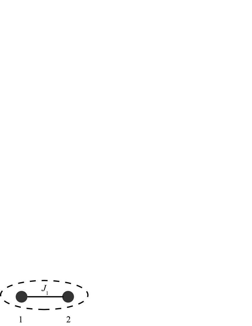
Figure 1: Dimer consists of two spin-$\frac{1}{2}$ particles.

We denote the eigenvectors of $\sigma_{z}$ as follows: $\sigma_{z}|+\rangle=|+\rangle$ and $\sigma_{z}|-\rangle=-|-\rangle$. Furthermore, we introduce the following vectors which are eigenvectors of $H_{\rm 1D}$: $|T_{+}\rangle=|++\rangle$, $|T_{0}\rangle=\frac{1}{\sqrt{2}}(|+-\rangle+|-+\rangle)$, $|T_{-}\rangle=|--\rangle$, and $|S_{0}\rangle=\frac{1}{\sqrt{2}}(|+-\rangle-|-+\rangle)$, where $|++\rangle$ denotes $|+\rangle\otimes|+\rangle$, and so on. The eigenvalues of $|T_{+}\rangle,|T_{0}\rangle,|T_{-}\rangle$, and $|S_{0}\rangle$ are $-2\omega+J_{1},-J_{1},2\omega+J_{1}$ and $-J_{1}$, respectively.

In case $\omega=J_{1}$, there exists $3$-fold degenerate lowest energy eigenvalue $-J_{1}$. The lowest eigenspace is spanned by the three eigenvectors $|T_{+}\rangle$, $|T_{0}\rangle$ and $|S_{0}\rangle$. The unique excited state is $|T_{-}\rangle$ and the energy difference between $|T_{-}\rangle$ and the ground state is $4J_{1}$.

In this paper, we choose $|0\rangle_{\rm L}=|T_{+}\rangle$ and $|1\rangle_{\rm L}=|T_{0}\rangle$ as basis vectors of the logical qubit. Namely, the coding space for a single qubit is $\mathcal{C}_{1}={\rm Span}\{|T_{+}\rangle,\,|T_{0}\rangle\}$. We note here that a qutrit may be implemented by using the three ground state eigenvectors. Although this coding is potentially interesting, it is beyond the scope of this paper.

III.2 Implementation of one-qubit gates

One-qubit gates are implemented by choosing $X$ in Eq. (2) as KarimipourMajd2005

$$X=i\bm{n}\Omega\cdot(\bm{\sigma}_{1}+\bm{\sigma}_{2}),$$ (10)

where $\bm{n}$ is a unit vector in $\mathbb{R}^{3}$, while $\Omega$ is a positive real number. It should be emphasized that undesired transitions into the irrelevant subspace ${\rm Span}\{|S_{0}\rangle\}$ do not occur for this choice of $X$. This is easily seen from the identity $(\sigma_{1a}+\sigma_{2a})|S_{0}\rangle=0$. We obtain the anti-Hermitian connection restricted to the coding space $\mathcal{C}_{1}$ as follows:

$$\left.A\right|_{\mathcal{C}_{1}}=i\Omega[n_{z}(I_{\rm L}+\sigma_{{\rm L}z})+\sqrt{2}(n_{x}\sigma_{{\rm L}x}+n_{y}\sigma_{{\rm L}y})].$$ (11)

where $\sigma_{{\rm L}x}=|T_{+}\rangle\langle T_{0}|+|T_{0}\rangle\langle T_{+}|$, $\sigma_{{\rm L}y}=-i(|T_{+}\rangle\langle T_{0}|-|T_{0}\rangle\langle T_{+}|)$, $\sigma_{{\rm L}z}=|T_{+}\rangle\langle T_{+}|-|T_{0}\rangle\langle T_{0}|$ and $I_{\rm L}=|T_{+}\rangle\langle T_{+}|+|T_{0}\rangle\langle T_{0}|$. Note that the presence of a closed loop in $\mathcal{M}$ is essential to obtain Eq. (11).

Using Eqs. (6) and (11), we find the unitary operator $\Gamma=e^{-i\Omega n_{z}}e^{-i\Omega[n_{z}\sigma_{{\rm L}z}+\sqrt{2}(n_{x}\sigma_{{\rm L}x}+n_{y}\sigma_{{\rm L}y})]}$. The condition $H_{\rm 1D}(1)=H_{\rm 1D}(0)$ is necessary for the closure of a loop in $\mathcal{M}$ comment . As for Eq. (10), this condition is obviously satisfied by taking $\Omega=\kappa\pi$ ($\kappa\in\mathbb{N}$), where $\kappa$ is interpreted as the winding number of a loop in $\mathcal{M}$.

Summarizing the above arguments, we find that $X$ given in Eq. (10) implements a single qubit holonomic gate

$$\Gamma^{(1)}_{\bm{m}}(\kappa) = e^{-i\kappa\pi n_{z}}\,e^{-i\theta_{\kappa}\bm{m}\,\cdot\bm{\sigma}_{\rm L}}.$$ (12)

where $\bm{m}=\frac{1}{\sqrt{2-n_{z}^{2}}}\left(\sqrt{2}n_{x},\,\sqrt{2}n_{y},\,n_{z}\right)$ and $\theta_{\kappa}=\kappa\pi\sqrt{2-n_{z}^{2}}$. In order that the holonomic quantum gate is non-trivial, the condition $[H_{\rm 1D},\,X]\neq 0$ must be satisfied. This condition is equivalent to $|n_{z}|\neq 1$.

Note that the set of the rotation angles $\theta_{\kappa}$ is discrete when $n_{z}$ is fixed, and hence it is impossible to vary $\theta_{\kappa}$ continuously in Eq. (12). Nevertheless, we can find a quantum gate that approximates the desired one with arbitrary accuracy provided that $\sqrt{2-n^{2}_{z}}$ is an irrational number comment2 .

III.3 Examples

III.3.1 Hadamard gate

The Hadamard gate, up to an irrelevant overall phase, is implemented by taking both $|\sin\theta_{\kappa}|=1$ and $\bm{m}=(1,0,1)/\sqrt{2}$ in $\Gamma^{(1)}_{\bm{m}}(\kappa)$. Note that $n_{z}=\sqrt{2/3}$ and $\theta_{\kappa}={2\kappa\pi}/{\sqrt{3}}$ for the choice of $\bm{m}$ and $|\sin\theta_{\kappa}|=1$ cannot be satisfied exactly for any $\kappa$. However we show that the Hadamard gate may be implemented with good accuracy for some $\kappa$. Figure 2 shows $\sin\theta_{\kappa}$ as a function of $\kappa$, from which we find that $|\sin\theta_{\kappa}|\simeq 1$ for $\kappa=3,10$ and $16$. It can be proved easily that the Hadamard gate can be implemented with arbitrary accuracy by choosing a proper $\kappa$.

Figure 2: $\sin\theta_{\kappa}$ as a function of $\kappa$.

III.3.2 Arbitrary elements of SU(2)

The holonomy $\Gamma^{(1)}_{(1,0,0)}(\kappa)$ is a quantum gate generating a rotation around the $x$-axis by an angle $\theta_{\kappa}=\sqrt{2}\kappa\pi$. Although the set of $\theta_{\kappa}$ is discrete, we can find $\kappa$ which satisfies $|(\theta-\theta_{\kappa})\,\,{\rm mod}\,\,2\pi|<\epsilon$ for arbitrary $\theta$ and $\epsilon$ comment2 . Figure 3 shows the points $(\cos\theta_{\kappa},\sin\theta_{\kappa})$ for $\kappa=0,1,\ldots,10$. The point $(1,\,0)$ corresponds to $\kappa=0$ (i.e., $X=0$), in which no gate operation is performed. Similarly, we obtain an approximate rotation around the $y$-axis with arbitrary accuracy by taking $\bm{m}=(0,\,1,\,0)$. Consequently, it is possible to implement an arbitrary element of SU(2).

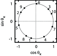
Figure 3: Rotation angles $\theta_{\kappa}=2\kappa\pi/\sqrt{3}$ in $\Gamma^{(1)}_{(1,\,0,\,0)}(\kappa)$ are plotted as points $(\cos\theta_{\kappa},\sin\theta_{\kappa})$ on the unit circle. The numbers in the figure indicate the values of $\kappa$.

IV Two-qubit gates

IV.1 Hamiltonian

A logical two-qubit system consists of two dimers. The Hamiltonian is

$$H_{\rm 2D} = H^{1}+H^{2},$$ (13)

where $H^{1}=-J_{1}\sigma_{1z}-J_{1}\,\sigma_{2z}+J_{1}\,\sigma_{1z}\sigma_{2z}$ and $H^{2}=-J_{2}\sigma_{3z}-J_{2}\,\sigma_{4z}+J_{2}\,\sigma_{3z}\sigma_{4z}$. Equation (13) is used as $H$ in Eq. (2). Here $H^{1}$ ($H^{2}$) is the Hamiltonian of a single dimer to which the first and the second (the third and the fourth) spins belong. We easily find the $9$-fold degenerate lowest eigenvalue $-J_{1}-J_{2}$.

We take the following coding space $\mathcal{C}_{2}$ for the logical two-qubit system: $\mathcal{C}_{2}={\rm Span}\{|T_{+}\rangle_{1}|T_{+}\rangle_{2},\,|T_{+}\rangle_{1}|T_{0}\rangle_{2},\,|T_{0}\rangle_{1}|T_{+}\rangle_{2},\,|T_{0}\rangle_{1}|T_{0}\rangle_{2}\}$. The vector $|T_{+}\rangle_{1}$ denotes the eigenvector $|++\rangle$ associated with $H^{1}$, for example.

IV.2 Controlled-$e^{i\theta Z}$ gate

We choose the following generator of the isospectral deformation in Eq. (2);

$$X = X^{1}+X^{2}+X^{1\text{-}2},$$ (14)

where $X^{1}=i\bm{n}_{1}\Omega_{1}\cdot(\bm{\sigma}_{1}+\bm{\sigma}_{2})$, $X^{2}=i\bm{n}_{2}\Omega_{2}\cdot(\bm{\sigma}_{3}+\bm{\sigma}_{4})$ and $X^{1\text{-}2}=iJ(\sigma_{1\,z}\sigma_{3\,z}+\sigma_{1\,z}\sigma_{4\,z}+\sigma_{2\,z}\sigma_{3\,z}+\sigma_{2\,z}\sigma_{4\,z})$. Here, $\bm{n}_{1}$ and $\bm{n}_{2}$ are unit vectors in $\mathbb{R}^{3}$, while $\Omega_{1}$, $\Omega_{2}$, and $J$ are positive real numbers. No undesired transitions into the non-coding space take place for this choice of $X$. We elaborate this point in Appendix B.

Let us find the corresponding anti-Hermitian connection with the following unit vectors $\bm{n}_{1}$ and $\bm{n}_{2}$;

$$\bm{n}_{1} = (0,\,0,\,1),$$ (15)

$$\bm{n}_{2} = \left(\sqrt{1-n^{2}_{2z}},\,\,0,\,\,n_{2z}\right),$$ (16)

$$n_{2z} = -\frac{J}{\Omega_{2}}.$$ (17)

We assume $\Omega_{2}>J$, which guarantees $[H_{2D},\,X]\neq 0$. Then, we obtain the following anti-Hermitian connection:

$$\left.A\right|_{\mathcal{C}_{2}} = i\big{[}\Omega_{1}I_{\rm L}\otimes I_{\rm L}+(\Omega_{1}+J)\sigma_{{\rm L}z}\otimes I_{\rm L}$$ (18)

$$+ \sqrt{2}\Omega_{2}n_{2x}I_{L}\otimes\sigma_{{\rm L}x}+J\sigma_{{\rm L}z}\otimes\sigma_{{\rm L}z}\big{]}.$$

Note here that $\Omega_{2}n_{2x}=\sqrt{\Omega^{2}_{2}-J^{2}}$.

The condition $e^{X}=\openone$ restricts the parameters as

$$\Omega_{2} = \kappa_{+}\pi\quad(\kappa_{+}\in\mathbb{N}),$$ (19)

$$\sqrt{\Omega_{2}^{2}+8J^{2}} = \kappa_{-}\pi\quad(\kappa_{-}\in\mathbb{N}),$$ (20)

$$\Omega_{1} = \kappa^{\prime}\pi\quad(\kappa^{\prime}\in\mathbb{N}).$$ (21)

Their derivation is given in Appendix B. It follows from Eqs. (19) and (20) that $\kappa_{-}>\kappa_{+}$ and $J=\frac{\pi}{2\sqrt{2}}\,\sqrt{\kappa_{-}^{2}-\kappa_{+}^{2}}$. Note that the assumption $\Omega_{2}>J$ is equivalent to $3\kappa_{+}>\kappa_{-}$.

As a result, we obtain a two-qubit gate

$$\Gamma^{(2)}(\bm{\kappa},\,\kappa^{\prime}) = (-1)^{\kappa^{\prime}}\,\Gamma^{\rm LU}(\bm{\kappa},\,\kappa^{\prime})\,\Gamma^{\rm C}(\bm{\kappa}),$$ (22)

where $\bm{\kappa}=(\kappa_{+},\,\kappa_{-})$. The local unitary gate $\Gamma^{\rm LU}(\bm{\kappa},\,\kappa^{\prime})$ is defined as

$$\Gamma^{\rm LU}(\bm{\kappa},\,\kappa^{\prime})=e^{-i(\kappa^{\prime}\pi+J)\sigma_{{\rm L}z}}\otimes e^{-i\nu\bm{k}\cdot\bm{\sigma}_{\rm L}},$$ (23)

where $\nu=\sqrt{2\kappa^{2}_{1}\pi^{2}-J^{2}}$ and $\nu\bm{k}=(\sqrt{2\kappa^{2}_{1}\pi^{2}-2J^{2}},\,0,\,J)$. The essential nonlocal operation is $\Gamma^{{\rm C}}(\bm{\kappa})$, which is a controlled-$e^{i\theta Z}$ gate and is given by

$$\Gamma^{\rm C}(\bm{\kappa})=|0\rangle_{\rm L}\langle 0|_{\rm L}\otimes I_{\rm L}+|1\rangle_{\rm L}\langle 1|_{\rm L}\otimes e^{i2J\sigma_{{\rm L}z}}.$$ (24)

Thus, $\Gamma^{(2)}(\bm{\kappa},\,\kappa^{\prime})$ followed by the local unitary gate $\Gamma^{\rm LU}(\bm{\kappa},\,\kappa^{\prime})^{\dagger}$ implements the controlled-$e^{i\theta Z}$ gate with $\theta=2J$

The rotation angle $2J$ in $\Gamma^{\rm C}(\bm{\kappa})$ is characterized by $\kappa_{+}$ and $\kappa_{-}$. We can, however, find $\kappa_{+}$ and $\kappa_{-}$ which satisfies $|(\theta-2J)\,\,{\rm mod}\,\,2\pi|<\epsilon$ for arbitrary $\theta$ and $\epsilon$ comment3 .

Figure 4: Rotation angle $2J$ in the controlled-$e^{i\theta Z}$, $\Gamma^{C}(\bm{\kappa})$. (a) The value of $2J$ with the unit of $\pi$ is plotted with respect to $\kappa_{-}$, when the fixed values of $\kappa_{+}$ are given. (b) The values of $\cos 2J$ and $\sin 2J$ are plotted as the points on the unit circle. The plotting marks are the same meaning as in Fig. 4(a).

We show the attainable values of $2J$ for the various sets of $(\kappa_{+},\,\kappa_{-})$ in Fig. 4 (a). Note that $(\kappa_{+},\,\kappa_{-})$ have to be chosen such that $\kappa_{+}<\kappa_{-}<3\kappa_{+}$ is satisfied. We calculate $(\cos 2J,\sin 2J)$ as in Fig. 4 (b). Thus, a tunable coupling control scheme, in which $J$ is controllable, is necessary to achieve various rotation angles in $\Gamma^{{\rm C}}(\bm{\kappa})$.

Alternatively, by repeating the above gate $n$ times, we can implement the controlled-$e^{i2nJ\sigma_{z}}$ gate. For an irrational $J$ and a given $\theta$, it is possible to find $n$ such that $|(2nJ-\theta)\ {\rm mod}\,2\pi|<\epsilon$ for an arbitrary $\epsilon$. In this way, one may implement the controlled-$e^{i\theta\sigma_{z}}$ gate with arbitrary precision. In particular, we can implement the controlled-Z gate, which is a constituent of the universal set of quantum gates, by taking $\theta=\pi/2$.

V Summary

We have constructed holonomic quantum gates using isospectral deformations of an Ising model Hamiltonian. These gates are the Hadamard gate, rotations around $x$- and $y$-axes and the controlled-$e^{i\theta Z}$ gate. The closure of the loop in the parameter manifold leads to a discrete set of gates. These gates are, however, dense in SU(2) and SU(4) and any one- and two-qubit gates can be implemented with arbitrary accuracy. A spin-chain model is a good candidate to implement holonomic quantum gates with the ground state eigenspace. We will propose a more feasible scheme based on the present analyses in our future work.

Appendix A Emulation of holonomic quantum gates

An exact solution of the Schrödinger equation is obtained when the Hamiltonian is deformed according to Eq. (2). Let us consider the Schrödinger equation in term of the dimensionless time $\tau$:

$$i\frac{d}{d\tau}|\psi(\tau)\rangle=TH(\tau)|\psi(\tau)\rangle,$$ (25)

where $H(\tau)=e^{X\tau}\,H\,e^{-X\tau}$. Introducing $|\phi(\tau)\rangle=e^{-X\tau}|\psi(\tau)\rangle$, we obtain the following equation for $|\phi(\tau)\rangle$:

$$i\frac{d}{d\tau}|\phi(\tau)\rangle=\left(-iX+H\right)|\phi(\tau)\rangle.$$ (26)

Accordingly, the time evolution operator at $\tau=1$ is

$$U(\tau=1)=e^{X}\,e^{-i(-iX+HT)}.$$ (27)

When the adiabatic approximation is valid and the initial state is in the lowest eigenspace, we obtain

$$U(\tau=1)P_{0}=e^{-iE_{0}T}\Gamma P_{0},$$ (28)

where $P_{0}$ is the projection operator on the lowest eigenspace. From Eqs. (27) and (28), we obtain

$$e^{X}\,e^{-i(-iX+HT)}P_{0}=e^{-iE_{0}T}\,\Gamma\,P_{0}.$$ (29)

The right hand side of Eq. (29) amounts to a holonomic quantum gates, up to the dynamical phase $e^{-iE_{0}T}$. The left hand side of Eq. (29) may be interpreted as implementation of the quantum dynamics by a pulse sequence. Equation. (29) provides a way how to emulate a holonomic gate $\Gamma$ with a series of pulses of $e^{-i(-iX+HT)}$ and $e^{X}$, although it may not be a genuine realization.

Appendix B Generator of isospectral deformation for two-qubit gates

Let us analyze the the generator of the isospectral deformation for two-qubit gates in Sec. IV.2. In this Appendix, we denote the eigenvector $|T_{+}\rangle_{1}|T_{+}\rangle_{2}$ simply as $|T_{+}T_{+}\rangle$, for example.

First, we focus on $X^{1}$ and $X^{2}$ in Eq. (14). We obtain

$$X^{1}=i\Omega_{1}\left(\begin{array}[]{ccc}2n_{1z}&\sqrt{2}(n_{1x}-in_{1y})&0\\ \sqrt{2}(n_{1x}+in_{1y})&0&0\\ 0&0&0\end{array}\right),\quad X^{2}=i\Omega_{2}\left(\begin{array}[]{ccc}2n_{2z}&\sqrt{2}(n_{2x}-in_{2y})&0\\ \sqrt{2}(n_{2x}+in_{2y})&0&0\\ 0&0&0\end{array}\right).$$ (36)

The matrix element $(X^{i})_{kl}$ corresponds to ${}_{i}\langle k|X^{i}|l\rangle_{i}$, where $|1\rangle_{i}=|T_{+}\rangle_{i}$, $|2\rangle_{i}=|T_{0}\rangle_{i}$, and $|3\rangle_{i}=|S_{0}\rangle_{i}$ $(i=1,\,2)$. One can easily find that $\langle T_{+}S_{0}|X^{1}|T_{+}T_{0}\rangle=0$, for example. This means that undesired transitions into the subspace irrelevant to quantum computation never occur under $X^{1}$ and $X^{2}$.

Next, let us consider $X^{1\text{-}2}$ in Eq. (14). The following observations are useful to calculate the matrix elements:

$$\sigma_{kz}|T_{+}\rangle_{i} = |T_{+}\rangle_{i},$$ (37)

$$\sigma_{kz}|T_{0}\rangle_{i} = (-1)^{k+1}|S_{0}\rangle_{i},$$ (38)

where $k=1,\,2$ for $i=1$ and $k=3,\,4$ for $i=2$.

Thus, we only have to consider five elements $\langle T_{+}T_{+}|X^{1\text{-}2}|T_{+}T_{+}\rangle$, $\langle T_{+}S_{0}|X^{1\text{-}2}|T_{+}T_{0}\rangle$, $\langle S_{0}T_{+}|X^{1\text{-}2}|T_{0}T_{+}\rangle$, $\langle S_{0}S_{0}|X^{1\text{-}2}|T_{0}S_{0}\rangle$, and $\langle S_{0}T_{0}|X^{1\text{-}2}|T_{0}S_{0}\rangle$. Note that one can easily calculate the other non-trivial elements (e.g., $\langle T_{0}T_{+}|X^{1\text{-}2}|S_{0}T_{+}\rangle$) from the anti-Hermitian property of $X^{1\text{-}2}$. The other elements which are related to the lowest eigenspace of $H_{2D}$ trivially vanish. As a result, we obtain the following results: $\langle T_{+}T_{+}|X^{1\text{-}2}|T_{+}T_{+}\rangle=i4J$ and $\langle T_{+}S_{0}|X^{1\text{-}2}|T_{+}T_{0}\rangle=\langle S_{0}T_{+}|X^{1\text{-}2}|T_{0}T_{+}\rangle=\langle S_{0}S_{0}|X^{1\text{-}2}|T_{0}S_{0}\rangle=\langle S_{0}T_{0}|X^{1\text{-}2}|T_{0}S_{0}\rangle=0$. As a result, all the matrix elements corresponding to the undesired transition to the irrelevant subspace vanish.

Finally, we calculate $e^{X}$ when the unit vectors $\bm{n}_{1}$ and $\bm{n}_{2}$ are given by Eqs. (15) and (16), respectively. We obtain

$$e^{X} = |T_{+}\rangle_{11}\langle T_{+}|\otimes e^{iY_{+}}+|T_{-}\rangle_{11}\langle T_{-}|\otimes e^{iY_{-}}$$ (39)

$$\quad+(|T_{0}\rangle_{11}\langle T_{0}|+|S_{0}\rangle_{11}\langle S_{0}|)\otimes e^{iY_{0}},$$

$$Y_{0} = \Omega_{2}\bm{n}_{2}\cdot(\bm{\sigma}_{3}+\bm{\sigma}_{4}),$$ (40)

$$Y_{\pm} = \pm 2\Omega_{1}\openone_{2}+\nu_{\pm}\bm{k}_{\pm}\cdot(\bm{\sigma}_{3}+\bm{\sigma}_{4}),$$ (41)

where $\nu_{+}=\Omega_{2}$, $\nu_{-}=\sqrt{\Omega^{2}_{2}+8J^{2}}$, and $\openone_{2}=|T_{+}\rangle_{22}\langle T_{+}|+|T_{0}\rangle_{22}\langle T_{0}|+|T_{-}\rangle_{22}\langle T_{-}|+|S_{0}\rangle_{22}\langle S_{0}|$. In particular, the values of $\nu_{\pm}$ is important for imposing the condition $e^{X}=\openone$. The unit vector $\bm{k}_{\pm}$ is given by $\nu_{\pm}\bm{k}_{\pm}=(\Omega_{2}n_{2x},\,0,\,\Omega_{2}n_{2z}\pm 2J)$. The condition $e^{X}=\openone$ implies $e^{iY_{0}}=\openone_{2}$ and $e^{iY_{\pm}}=\openone_{2}$. The condition $e^{iY_{0}}=\openone_{2}$ implies there is $\kappa_{+}\in\mathbb{N}$ such that $\Omega_{2}=\kappa_{+}\pi$; this requirement is equivalent to Eq. (19). Similarly, if Eqs. (20) and (21) are satisfied, then we obtain $e^{iY_{\pm}}=\openone_{2}$.

References

- (1) F. Wilczek and A. Zee, Phys. Rev. Lett. 52, 2111 (1984).
- (2) M. Nakahara, Geometry, Topology and Physics 2nd ed. (CRC Press, Boca Raton, London and New York, 2003).
- (3) P. Zanardi and M. Rasetti, Phys. Lett. A 264, 94 (1999).
- (4) K. Fujii, J. Math. Phys. 41, 4406 (2000).
- (5) K. Fujii, Rep. Math. Phys. 48, 75 (2001).
- (6) A. O. Niskanen, M. Nakahara, and M. M. Salomaa, Phys. Rev. A 67, 012319 (2003).
- (7) S. Tanimura, D. Hayashi, and M. Nakahara, Phys. Lett. A 325, 199 (2004).
- (8) V. Karimipour and N. Majd, Phys. Rev. A 70, 012320 (2004).
- (9) S. Tanimura, M. Nakahara, and D. Hayashi, J. Math. Phys. 46, 022101 (2005).
- (10) P. Solinas, P. Zanardi, and N. Zanghi, Phys. Rev. A 70, 042316 (2004).
- (11) J. Pachos and S. Chountasis, Phys. Rev. A 62, 052318 (2000).
- (12) L .-M. Duan, J. I. Cirac, and P. Zoller, Science 292, 1695 (2001).
- (13) A. Recati, T. Calarco, P. Zanardi, J. I. Cirac, and P. Zoller, Phys. Rev. A 66, 032309 (2002).
- (14) J. Pachos, Phys. Rev. A 66, 042318 (2002).
- (15) L. Faoro, J. Siewert, and R. Fazio, Phys. Rev. Lett. 90, 028301 (2003).
- (16) H. Goto and K. Ichimura, Phys. Rev. A 75, 033404 (2007).
- (17) V. Karimipour and N. Majd, Phys. Rev. A 72, 052305 (2005).
- (18) T. Kato, J. Phys. Soc. J. 5, 435 (1950); A. Messiah, Quantum Mechanics (Dover, New York, 1999), Chap. XVII.
- (19) It seems that the condition is not properly taken into account in Ref. KarimipourMajd2005 . They take , for a one-qubit gate and , for the Hadamard gate. Consequently, the coefficient of in is , which shows .
- (20) If an irrational number is given, the set is dense in the interval , where and is the greatest integer that is less than or equal to HardyWright1978 . Accordingly, for arbitrary and , there is such that .
- (21) H. Weyl, Math. Ann. 77, 31 (1916); G. H. Hardy and E. M. Wright, An Introduction to the Theory of Numbers (Oxford University Press, New York, 1979) 5th ed, Chap. XXIII.
- (22) Let us first put and (), where the value of is an irrational number; for example, when . Next, we redefine the values of and as follows: and , where . Note that those values satisfy and , because and . Thus, the rotation angle is . Therefore, we can find a proper such that approximates a given rotation angle with arbitrary accuracy comment2 .