Atmospheric Circulation of Hot Jupiters: A Shallow Three-Dimensional Model
Abstract
Remote observing of exoplanetary atmospheres is now possible, offering us access to circulation regimes unlike any of the familiar Solar System cases. Atmospheric circulation models are being developed to study these new regimes but model validations and intercomparisons are needed to establish their consistency and accuracy. To this end, we present a simple Earth-like validation of the pseudo-spectral solver of meteorological equations called IGCM (Intermediate General Circulation Model), based on Newtonian relaxation to a prescribed latitudinal profile of equilibrium temperatures. We then describe a straightforward and idealized model extension to the atmospheric flow on a hot Jupiter with the same IGCM solver. This shallow, three-dimensional hot Jupiter model is based on Newtonian relaxation to a permanent day-night pattern of equilibrium temperatures and the absence of surface drag. The baroclinic regime111Contours of pressure and density are misaligned in a baroclinic flow, while they are aligned in a barotropic flow. Strongly baroclinic flows are susceptible to baroclinic instabilities which, in essence, are slanted versions of convection (see the review by Showman et al., 2008). of the Earth’s lower atmosphere is contrasted with the more barotropic regime of the simulated hot Jupiter flow. For plausible conditions at the 0.1-1 bar pressure level on HD 209458b, the simulated flow is characterized by unsteadiness, subsonic wind speeds, a zonally-perturbed superrotating equatorial jet and large scale polar vortices. Violation of the Rayleigh-Kuo inflexion point criterion on the flanks of the accelerating equatorial jet indicates that barotropic (horizontal shear) instabilities may be important dynamical features of the simulated flow. Similarities and differences with previously published simulated hot Jupiter flows are briefly noted.
1 Introduction
Since the first discoveries of extrasolar giant planets around nearby sun-like stars with Doppler velocimetry (Mayor & Queloz 1995; Marcy & Butler 1996), extrasolar planet research has experienced a spectacular series of observational breakthroughs. In recent years, progress has been particularly rapid with a subset of close-in extrasolar planets found to transit the disk of their host star (e.g., Charbonneau, 2008; Deming, 2008).
The first transit observation of a hot Jupiter (Charbonneau et al. 2000; Henry et al. 2000) has been followed by many such measurements, including a growing number of new close-in planet discoveries based on transit searches (e.g., Torres et al., 2008). For the brightest nearby systems with transiting planets, this has also enabled the detection of the planetary thermal flux occulted at secondary eclipse (e.g., Deming et al. 2005, 2006; Charbonneau et al. 2005; Harrington et al. 2007), the detection of day/night temperature variations through IR phase curve monitoring (e.g. Harrington et al. 2006; Knutson et al. 2007, 2008b; Cowan et al. 2007), IR spectral measurements (Grillmair et al. 2007; Richardson et al. 2007; Knutson et al. 2008a) as well as a variety of additional constraints based on transit spectroscopic studies (Tinetti et al. 2007; Ehrenreich et al. 2007; Swain et al. 2008; Barman 2007; Redfield et al. 2008; Pont et al. 2008). Overall, these results have contributed to a shift in focus from the detection of extrasolar planets to the characterization of their physical atmospheric properties (e.g., Seager et al., 2005; Burrows et al., 2006; Marley et al., 2007; Fortney & Marley, 2007; Barman, 2008; Burrows et al., 2008).
The need to interpret these astronomical data reliably, so as to infer the physical conditions present in distant exoplanetary atmospheres, has also fueled a growing atmospheric modeling effort. While plane-parallel radiative models have been the tools of choice to interpret these data until now, they are likely insufficient in the case of hot Jupiter/Neptune atmospheres. Indeed, due to their short orbital separations, all these exoplanets are expected be tidally-locked to their parent star (or, in some cases, pseudo-synchronized). Tidally-locked planets are subject to an unusual situation of permanent, asymmetric day/night radiative forcing, leading to heat redistribution by atmospheric motions. Current data on hot Jupiters already indicate that existing one-dimensional radiative transfer models fail to capture the multi-dimensional nature of this atmospheric regime (e.g., Seager et al. 2005; Knutson et al. 2007; 2008b; Fortney et al. 2006) and, when included, the effects of atmospheric heat redistribution are usually accounted for only indirectly (e.g., Iro et al., 2005; Seager et al., 2005; Barman, 2008; Burrows et al., 2008; Fortney et al., 2008). To adequately address this circulation regime and interpret the growing data set, multi-dimensional, coupled radiation-hydrodynamics models of these atmospheres are required (see the review by Showman et al., 2008).
Hot Jupiters have high atmospheric temperatures, slow rotation rates and an unusually permanent pattern of asymmetric day/night radiative forcing. Recognizing that this constitutes an interesting problem in atmospheric dynamics, several groups have explored plausible circulation regimes on these planets using different modeling approaches and assumptions (Showman & Guillot, 2002; Cho et al., 2003; Menou et al., 2003; Cooper & Showman, 2005, 2006; Langton & Laughlin, 2007; Cho et al., 2008; Dobbs-Dixon & Lin, 2008; Langton & Laughlin, 2008; Showman et al., 2008). These investigations have exhibited significant diversity in flow results, for which there currently is no simple unifying explanation (see the discussion in Showman et al., 2008).
Atmospheres in motion are non-linear, presumably turbulent flows. In addition, radiatively active species in an atmosphere are advected by the flow and in doing so non-linearly couple the flow to its effective source of radiative forcing. Simulated atmospheric flows are thus generally expected to be sensitive to various numerical and physical details of any specific implementation. In the exoplanetary context, with rather limited direct information on the atmospheres studied, this means that simple parameterized models isolating key features of the simulated flow are important in helping us understand the general behavior of remote atmospheric flows. With this in mind, we present here idealized atmospheric models which emphasize dynamical aspects under linear forcing conditions. These simplified models do not address any detailed aspect of the radiative or chemical structure of the atmospheres under consideration.
In general, different numerical implementations of a specific atmospheric problem will not lead to identical results. For this reason, model validations and inter-comparisons are standard practices in atmospheric science. This is particularly true of the complex hydrodynamic solvers known as dynamical cores (e.g., Held & Suarez, 1994). The development of dynamical cores to solve the equations satisfied by an hydrostatic atmosphere in motion has been a major enterprise. Dynamical cores currently used in meteorological and climate models are the results of years of refinements to guarantee stability, efficiency, and accurate conservation of mass, momentum and energy (e.g., Hoskins & Simmons, 1975). In the exoplanetary context, different modeling groups have used various hydrodynamic solvers. Some are new and little tested while others are old, well-tested but only validated under conditions appropriate for Solar System planetary atmospheres. As a result, intercomparisons and validations of dynamical cores on idealized atmospheric problems tailored for exoplanets will be important in the future to assess, both qualitatively and quantitatively, how reliable our interpretations of exoplanetary data can be.
As a first step in this direction, we present here a simple Earth-like validation of the IGCM dynamical core (in §3), followed by a direct extension of this model to the atmospheric flow on a hot Jupiter (in §4).
2 The IGCM Dynamical Core
The IGCM dynamical core has its origins in the development of accurate numerical solvers for meteorological studies (Hoskins & Simmons, 1975). It is a well tested and documented solver, which has been used for studies as diverse as the climate of the Earth (Forster et al., 2000), the meteorology of Mars (Joshi et al., 1995; Collins & James, 1995) and the atmospheric circulation regime of tidally-locked terrestrial exoplanets (Joshi et al., 1997). We summarize the main features of this dynamical solver here.
2.1 Equations of Motion
We consider a coordinate system rotating with the same angular velocity, , as the planet. Longitude ranges from to in the eastward direction and latitude ranges from at the south pole to at the north pole. From the general fluid equations satisfied by an inviscid ideal gas, one derives the primitive equations of meteorology in the traditional approximation, which are satisfied on large horizontal scales222The primitive equations cease to be satisfied by motions with horizontal scales approaching the atmospheric vertical scale height (e.g., Holton 1992; Vallis 2006). by a hydrostatic atmosphere in motion. Using pressure, , as the vertical coordinate, equations for the conservation of momentum, mass and energy can be written, respectively,
| (1a) | |||||
| (1b) | |||||
| (1c) | |||||
| (1d) | |||||
| where the Lagrangian derivative is | |||||
| (1e) | |||||
is the (eastward, northward) horizontal velocity in the rotating frame, is the planetary radius and is the vertical “velocity.” The geopotential , where is the height above a fiducial pressure surface and is the gravitational acceleration, which is assumed to be constant and includes the contribution from the centrifugal acceleration. The unit vector is normal to the “planetary surface.” The Coriolis parameter is the projection of the planetary vorticity vector, , onto . The operator is the horizontal gradient on a constant- surface. In the energy equation, is the heat capacity of the atmospheric gas at constant pressure and is the diabatic heating/cooling rate. The above equations are closed with the ideal gas law, , as the equation of state, where is the atmospheric perfect gas constant. The validity of the primitive equations in the traditional approximation for the study of hot Jupiter atmospheric flows has been discussed, for instance, by Showman et al. (2008) and Cho et al. (2008).
The IGCM dynamical core solves these equations in a form that involves the vorticity and divergence of the horizontal flow. Using scaled units of length (), time333All times are subsequently quoted in units of a planetary day equal to . () and temperature (), as well as rescaled zonal and meridional velocities
the horizontal momentum equations specifically solved are the equation for the vertical component of absolute vorticity, ,
| (2) |
and the equation for the horizontal divergence, ,
| (3) |
where
Conservation of energy is expressed via the temperature equation
| (4) |
where the temperature is decomposed into an arbitrary (constant) reference value, , around which the anomaly, , is calculated. Conservation of mass is expressed via an equation for the vertically integrated “surface” pressure,
| (5) |
where is the pressure at the bottom model level, due to the entire weight of the overlaying atmosphere. Momentum balance in the vertical satisfies the same hydrostatic equation as before,
| (6) |
In all the above equations, the vertical pressure coordinate is used (). These five equations are the exact same ones as originally solved by Hoskins & Simmons (1975), except for the various additional terms entering the vorticity, divergence and temperature equations.
2.2 Forcing, Friction and Hyperdissipation
Our IGCM implementation contains linear prescriptions for temperature relaxation as well as drag on the vorticity and divergence fields. Newtonian relaxation of the temperature field to a prescribed equilibrium temperature profile, , on a characteristic radiative time , corresponds to
| (7) |
in equation (4). This linear temperature relaxation scheme is a very simplified form of atmospheric forcing which encapsulates all the unspecified chemical-radiative physics in the modeled atmosphere. Rayleigh drag on the horizontal flow field, on a characteristic friction time , corresponds to
| (8) | |||||
| (9) |
in equations (2) and (3), respectively. (Note that friction is only applied to the relative vorticity field.)
In this work, Rayleigh drag is used as a simple parameterization of surface friction in the Earth-like model only, while Newtonian relaxation is used as the unique form of forcing in all models. The vertical profile of equilibrium temperature used has two regions, a lower atmosphere (troposphere) where temperature decreases with height at a fixed rate, and an upper atmosphere (stratosphere) which is vertically isothermal. The specific relaxation temperature profile adopted in all the models has the form
| (10) |
where is the height above the lowest “surface” level, is the “surface” temperature, is the lapse rate ( ) in the tropospheric region, is the height at which one enters the stratospheric region and is a temperature offset used to smooth out the transition between the finite tropospheric lapse rate and the isothermal stratosphere.
Differential heating and cooling of atmospheric regions around the planet drives atmospheric motions. In addition to the vertical dependence in equation (10), one must also specify the latitudinal and longitudinal dependence of the temperature relaxation profile. In our models, the three-dimensional equilibrium temperature is given by
| (11) |
where
is a height-dependent damping factor applied in the troposphere () to gradually reduce the latitudinal and longitudinal temperature differential over the vertical extent of the troposphere. In the stratosphere, this horizontal temperature differential is set to zero: . The correspondence between and levels is obtained by vertical integration of the hydrostatic balance equation (Eq. [6]). The latitudinal and longitudinal dependence of the relaxation temperature profiles, , are specified separately for the Earth-like and hot Jupiter models in § 3 and § 4 below.
When using the primitive equations, one assumes that effects on small scales, which are not adequately described by the equations, nor resolved numerically, can be parameterized within the framework of the large-scale dynamics. In particular, in a turbulent two-dimensional flow, enstrophy444Enstrophy is the “vortical energy” of the flow, defined by , where is the relative vorticity (parallel to the vertical direction ). is known to cascade to small scales, where three-dimensional effects eventually become important (e.g., Pedlosky, 1987). In the absence of explicit dissipation in a numerical atmospheric model, enstrophy accumulates at the smallest resolved scales, in a process known as spectral blocking, with ever growing numerical errors. It is thus standard practice in atmospheric science to introduce hyperdissipation terms in the equations solved to alleviate the spectral blocking problem (e.g., Stephenson, 1994).
In the IGCM, hyperdissipation terms are introduced in the vorticity, divergence and temperature equations,
| (12) | |||||
| (13) | |||||
| (14) |
where is an integer. (Note that hyperdissipation is only applied to the relative vorticity, .) Hyper-laplacian operators guarantee that only scales close to the smallest resolved features are selectively chosen for diffusion. The case , which would correspond to a regular diffusion operator, is considered to be too widely dissipative for what are effectively inviscid planetary atmospheres.
It should be noted that hyperdissipation is a numerical tool with intrinsic limitations. It is not supported by any fundamental theory and it may well miss some of the “reverse” interactions occurring between small and large horizontal scales in a turbulent atmospheric flow. There is no rigorous way to chose the magnitude or the order of hyperdissipation in a given model (e.g., McVean, 1983) and different choices have typically been made by different modeling groups in Earth atmospheric studies (e.g., Stephenson, 1994). In the context of exoplanet atmospheric modeling, with a priori unknown circulation regimes, hyperdissipation choices should probably be considered as important free parameters of the models. In keeping with standard practice (McVean, 1983; Stephenson, 1994), we use a highly scale-selective scheme and a dissipation rate adjusted with horizontal resolution so that structures on the smallest resolved scales are dissipated in a fraction ( – ) of a planetary day.
2.3 Numerical Solutions
The IGCM solves equations (2)–(6) with the semi-implicit pseudo-spectral method (Hoskins & Simmons, 1975). The equations are solved in spectral space horizontally and with a finite difference scheme in the vertical. A standard decomposition in spherical harmonics is used with triangular mode truncation (Orszag, 1970; Eliassen et al., 1970; Washington & Parkinson, 1995). The pseudo-spectral method is well adapted to problems with spherical geometry and thus does not require any special treatment at the poles. The vertical finite difference scheme is based on the formulation of Simmons & Burridge (1981), which conserves angular momentum and energy exactly. As is usually the case with this formulation, total atmospheric mass is not conserved by the vertical scheme but is instead corrected for at each time-step. Vertical levels are linearly spaced in . In what follows, model resolutions are reported as TL, which corresponds to spectral modes in longitude, half that in latitude, and vertical levels. Time integration is performed with a semi-implicit leapfrog scheme, followed by a Robert-Asselin filter to control time splitting (Hoskins & Simmons, 1975; Forster et al., 2000). A significant advantage of the semi-implicit method is that it solves gravity wave propagation in an implicit manner. Larger time steps are thus possible since CFL stability is determined by advection, rather than the speed of gravity waves.
Boundary conditions are applied only at the top () and bottom () of the numerical domain, where is imposed. By default, this corresponds to free-slip boundary conditions for the horizontal flow. All our models are started at rest, with a temperature profile satisfying everywhere the equilibrium profile in equation (10). A small amount of noise is introduced to break flow symmetries.
2.4 Flow Representations
There are various ways to represent a three-dimensional atmospheric flow. In the interest of clarity and conciseness, we only show cylindrical maps and zonally-averaged contour plots. Our temperature and velocity maps use Miller cylindrical projections, centered on the equator (and the substellar point, at , in the case of the hot Jupiter model). In some cases, only a subset of all velocity vectors are shown, for better rendering. We also present zonally-averaged contours of zonal velocity, , and temperature, . These were obtained by performing the longitudinal average
| (15) |
where or .
3 Earth-Like Model
Our Earth-like model comes as a default implementation of the IGCM solver. It has many similarities with the control run described by James & Gray (1986). To capture in a simple way Earth’s annual mean conditions, a meridional gradient of relaxation temperatures is imposed, such that
| (16) |
where the equator-pole temperature difference is set to K. Parameters for the vertical relaxation profile, in equation (10), are chosen to capture approximately Earth’s typical radiative-convective conditions. For simplicity, a single value for the radiative relaxation time, planet days, is adopted throughout the atmosphere. Rayleigh drag with a friction time planet day is applied to the lowest model layer only. There is no account of seasonal variations or topography in the model. Stratospheric conditions are rather poorly captured. The complete list of parameters of our Earth-like model with T42L15 resolution is provided in Table 1.
This model also share strong similarities with the classic benchmark calculation of Held & Suarez (1994) for dynamical core validations. A significant difference with the Held-Suarez benchmark is that the variations of and values with location in the atmosphere in that model are reduced to single values in the simpler model presented here. Our Earth-like model may thus be considered as a crude version of the Held-Suarez benchmark, with a reduced number of free parameters.
The main features of Earth’s general atmospheric circulation and the ability of idealized models such as the Held-Suarez benchmark to reproduce them with reasonable accuracy are well known (e.g., Held & Suarez, 1994). The key features of the tropospheric circulation, at bar () levels, are: (i) an axisymmetric meridional circulation via Hadley cells extended from the equator to approximately in latitude, which efficiently reduce meridional temperature gradients in that region, (ii) strong baroclinic activity at mid-latitudes, with typically large scale baroclinic eddies spread in longitude along a “storm track,” (iii) a zonal circulation at the surface which is characterized by easterly (westward) trade winds in subtropical latitudes, westerlies (eastward wind) in mid-latitudes and weak easterlies near the poles, (iv) a westerly component of the zonal wind increasing with height at all latitudes, until localized wind maxima known as the jet streams are reached at the bar () level, with peak winds at – latitude.
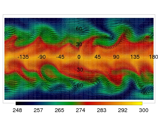
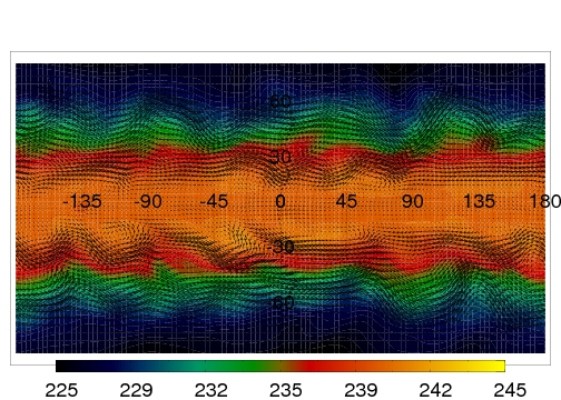
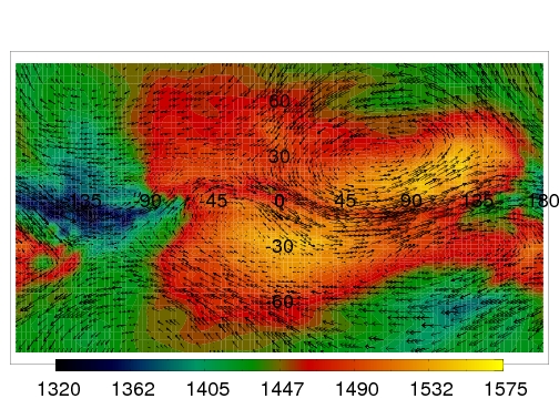
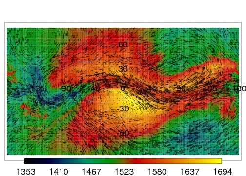
Figures 1 and 2 illustrate how our simple Earth-like model qualitatively reproduces this general circulation regime. While time averages over hundreds of planet days are traditionally used to characterize the flow in the Held-Suarez benchmark (Held & Suarez, 1994), we have chosen to present snapshots of the atmospheric flow for simplicity and to facilitate comparisons with the hot Jupiter model presented below. Figure 1 shows temperature and velocity maps at planet day 150 in the Earth-like model. The top panel exemplifies the strong baroclinic activity that characterizes mid-latitudes, shown here in the bottom model layer at the ( bar) level. The bottom panel exemplifies the reduced baroclinic activity and the formation of jet streams that characterize the upper troposphere, shown here at the ( bar) level.
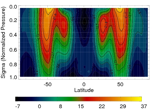
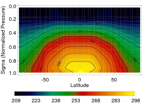
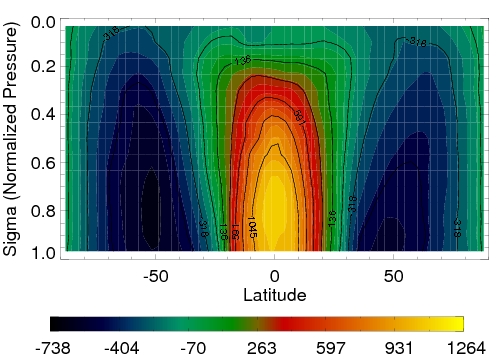
Figure 2 shows zonally-averaged contours of zonal wind speeds ( in m s-1; top panel) and temperature ( in K; bottom panel) for the same Earth-like flow at planet day 150 as shown in Figure 1. While the contours reproduce the main qualitative features of the Held-Suarez benchmark calculation (see Fig. 2 in Held & Suarez, 1994), quantitative discrepancies emerge, most notably in the extremas of wind speeds and in the detailed shape of the zonal wind structure (with jet stream cores incorrectly pushed against the top layer in our model). We attribute these differences to the simpler nature of Newtonian forcing and Rayleigh drag in our model, different relaxation profiles and our focus on a flow snapshot rather long-term averages. Similarly, a comparison of the contours shown in the lower panel of Figure 2 with the corresponding Figure 1c in Held & Suarez (1994) reveals broad qualitative agreement (e.g., flattened equatorial contours) but also quantitative discrepancies. These discrepancies can be partly attributed to the different vertical profiles of relaxation temperature adopted here and in Held & Suarez (1994).
Rather than focusing on a strict reproduction of the Held-Suarez benchmark results, which is of limited interest for a well-tested code like the IGCM solver (see, e.g., the climatology of Forster et al., 2000), our simple Earth-like model may offer interesting insight into important issues of model parameterizations and target accuracies for exoplanet atmospheric circulation studies. By comparison with a somewhat higher complexity model like the Held-Suarez benchmark calculation, it provides a measure of the ability of strongly parameterized models to successfully reproduce the main qualitative features of an atmospheric circulation regime like that on Earth. We note, however, that in both our model and the Held-Suarez benchmark, parameters were adjusted a posteriori to reproduce a known circulation regime. By contrast, circulation regimes are a priori unknown on exoplanets and it may be difficult to determine from first principles the temperature relaxation profiles and relaxation times needed to adequately drive or drag the flow on a remote planet. On the other hand, it could also be that qualitative agreement at a level comparable to that achieved by our simple Earth-like model turns out to be sufficient to interpret with confidence typical remote astronomical observations of exoplanets. The issue of target accuracies for reliable exoplanet data interpretation has received little attention until now. We will simply note here that, in addition to validations and inter-comparisons, parameter-space explorations with simple atmospheric circulation models may be important ingredients of an effective strategy to address this data interpretation challenge.
4 Shallow Hot Jupiter Model
To capture the permanent day–night forcing conditions present on a tidally-locked hot Jupiter, our IGCM solver has been modified to permit horizontal gradients of relaxation temperatures of the form
| (17) |
which places the substellar point at . In the specific hot Jupiter model presented here, the equator-pole temperature difference is set to K, which corresponds to a full day-night temperature difference of K. The amplitude of this day-night temperature forcing, which is an important free-parameter of our model, is comparable to the corresponding forcing amplitude at the bar level in the circulation model of Cooper & Showman (2005). A relatively steep, linear dependence of the equilibrium relaxation temperature with the cosine of the angle away from the substellar point has been adopted because it accounts for the extra atmospheric depth crossed by radiation at inclined angles and is broadly consistent with detailed radiative transfer calculations (e.g., Showman et al., 2008).
Parameters for the vertical relaxation profile, in equation (10), are chosen to match approximately the profile of Iro et al. (2005) in the - bar region for HD 209458 b, with a constant lapse rate K m-1 and no stratosphere. A significant feature of our vertical relaxation profile is that the day-night temperature differential asymptots to zero in the uppermost modeled layers, like it does in the Earth-like model (see Eqs. [11–2.2]). While this choice facilitates a direct comparison of circulation regimes between the Earth-like model (with meridional forcing) and the hot Jupiter model (with hemispheric forcing), it may also be a poor assumption for a hot Jupiter atmosphere. More realistically, the day-night temperature differential would extend to layers higher up in the atmosphere (beyond those modeled), with the possible existence of a stratosphere depending on the presence of an absorbing compound such as TiO/VO or Sulfur (Hubeny et al., 2003; Burrows et al., 2007; Fortney et al., 2008; Spiegel et al., 2009; Zahnle et al., 2009).
We adopt a single value for the radiative relaxation time, planet day s, to match the radiative timescale at 1 bar from Iro et al. (2005). While the radiative times are expected to vary substantially with depth in hot Jupiter atmospheres, a single value, like in our Earth-like model, is the simplest acceptable form of radiative forcing in a shallow atmospheric model such as ours. No Rayleigh drag is implemented. All the other parameters are chosen appropriately for the hot Jupiter HD 209458 b. The complete list of parameters of this idealized hot Jupiter model with T42L15 resolution is provided in Table 1. We emphasize that the model is quite shallow in the sense that only 1–2 vertical levels are present above the level (given the linear- grid and vertical resolutions used) and that absolutely no account is made of deeper atmospheric layers present below the 1 bar pressure level (which bounds our model at ). Despite its great simplicity, a clear advantage of this shallow hot Jupiter model is that it is a direct extension of our Earth-like model setup to the case of a hot Jupiter atmospheric flow and thus permits straightforward comparisons between the two simulated circulation regimes.
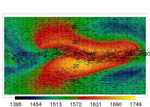
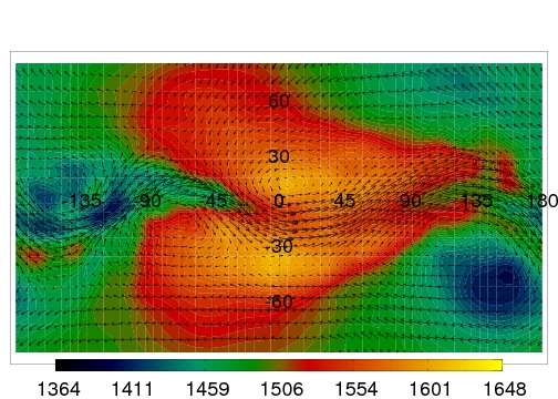
Figure 3 shows temperature and velocity maps at planet day 100 in the hot Jupiter model, at the (top panel) and (bottom panel) levels. The temperature fields and particularly the velocity fields share strong similarities at these two levels. This vertical flow alignment, which persists throughout the various modeled layers, together with the lack of any identifiable baroclinic eddies, is characteristic of a barotropic flow regime (e.g., Cho et al., 2003; Menou et al., 2003; Cho et al., 2008). The flow is characterized by a zonally-perturbed superrotating equatorial wind, flanked by dynamically active vortices, counter-jets at mid-latitudes and the presence of large scale polar vortices. Advection of heat away from the substellar point, at , occurs both eastward in the equatorial regions and westward in mid-latitudes, where the counter-jets are present.
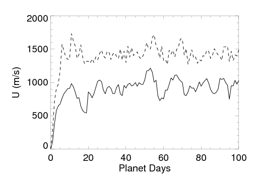
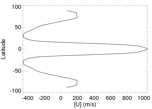
Figure 4 offers another view of the circulation regime in this shallow hot Jupiter model with zonal averages of the zonal wind velocity () at planet day 100. Over nearly the entire vertical extent of the model layer, the flow exhibits the broad super-rotating (eastward) equatorial wind and slower westward counter-jets at mid-latitudes. Maximum wind speeds are m s-1 and zonal averages are m s-1. These values are well below corresponding sound speeds, which range from to km s-1 from top to bottom of the modeled region.
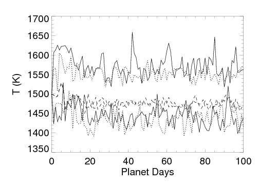
Various diagnostics can be used to verify that the flow has reached a stationary state with respect to the imposed forcing. We have performed extended runs for up to several hundred planetary days and have found stationary conditions for the shallow hot Jupiter model under consideration. To illustrate this, Figure 5 shows the time evolution over 100 planet days of representative velocities and temperatures at various horizontal locations on the model level. The zonal average and maximum values of the zonal velocity along the equator are shown in the top panel as solid and dashed lines, respectively. After a rapid acceleration phase lasting – planet days, a flow stationary state is reached at planet day , with significant fluctuations. Throughout this evolution, flow velocities remain subsonic. In the bottom panel of Figure 5, the corresponding evolution of temperatures is shown at the sub- and antistellar points (top and bottom solid lines, respectively), at the east and west equatorial limbs (top and bottom dotted lines, respectively) and at the north and south poles (two dashed lines). Despite eastward heat advection at the equator, which results in comparable temperatures at the east equatorial limb and the substellar point, temperatures are far from being horizontally homogeneous. Note in particular that temperatures around the planetary limb (dashed and dotted lines) represent a diverse range of physical conditions even on a fixed () pressure level (see also Fig. 3).
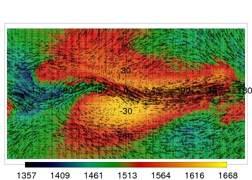
We have found that these results are broadly confirmed at different, and in particular higher, model resolutions. Figure 6 presents a specific test of numerical convergence for our results. Temperature and velocity maps at planet day 100 are shown for the same shallow hot Jupiter model as before, except that reduced and enhanced numerical resolutions were used, both horizontally and vertically. The top panel shows a map at the level in a T21L5 model. The bottom panel shows a corresponding map, at the level, in a T170L20 model. Values of the hyperdissipation coefficient were adjusted to and m8 s-1 in these T21L5 and T170L20 models, respectively. The overall similarity of these temperature and velocity maps, as well as other flow attributes (e.g., zonal wind contours), indicates that good convergence is already achieved around T31L10 to T42L15 resolution. Even the T21L5 flow shares many of the global attributes of higher resolution simulated flows.
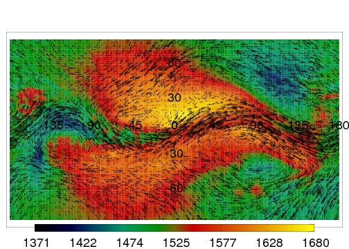
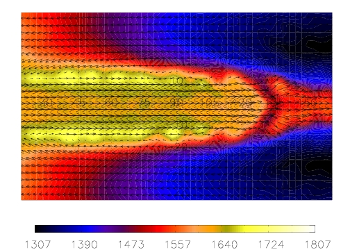
As mentioned earlier, the zonally-perturbed equatorial wind and its flank vortices are dynamical features of the simulated flow. Figure 7 illustrates the flow unsteadiness with two successive temperature and velocity maps at planet days 97 and 98 in a T85L20 version of our shallow hot Jupiter model (with adjusted to m8 s-1). The maps are shown at the level. While this particular example was chosen to exhibit clear temperature and flow field variability over one planet day, dynamical variability is a general property of the simulated flow (see fluctuations in Fig. 5). Nevertheless, we find that the displaced anticyclonic polar vortices that emerge in this hot Jupiter model do not experience systematic longitudinal translations, nor are they close to geostrophic balance, like the cyclonic circumpolar vortices discussed by Cho et al. (2003, 2008). Instead, the polar vortices in the present model appear to be strongly tied to the imposed day-night forcing and show only limited excursions away from their preferred night-side location, somewhat eastward of the anti-stellar point (see Figs. 3, 6 and 7).
The wind acceleration episode apparent in Figure 5 must be important in determining the nature of the stationary regime eventually achieved by the forced flow. We have found evidence that barotropic instabilities play a role in shaping the dynamical nature of this flow. During the first few planet days in our hot Jupiter model, we observe the acceleration of a zonal eastward wind in the equatorial regions and westward counter-jets at mid-latitudes. This situation is very reminiscent of the counter-acceleration caused by meridional Rossby wave transport that occurs in the idealized momentum-forced flow discussed by Cho et al. (2008) in the context of the equivalent-barotropic formulation (see their Fig. 17). Figure 8 shows a temperature and velocity map at planet day 5 and level in our T42L15 hot Jupiter model. In contrast with previous maps, this one zooms in a specific region along the equator, restricted to in longitude and in latitude. In this region, the flow exhibits strong horizontal (zonal) shear, as well as small scale velocity and temperature disturbances along the leading edge of the equatorial jet. Subsequently, we observe a rapid thinning of the jet, a breaking of equatorial symmetry by planet day - and the emergence of a broader, wavy equatorial wind, as shown for instance in Figure 3.
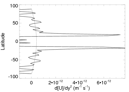
Figure 9 suggests that horizontal shear (= barotropic) instabilities are important dynamical ingredients of the sequential flow evolution we have just described. The latitudinal profile of zonally-averaged zonal wind velocity, , is shown in the top panel, while its second-order meridional derivative, , is shown in the bottom panel, for the same planet day 5 and level flow as in Fig. 8. Although necessary and sufficient conditions for the development of barotropic (horizontal shear) instabilities are generally not known, the Rayleigh-Kuo inflexion point criterion provides a useful necessary condition, which accounts for the stabilizing influence of the planetary vorticity (Kuo, 1949; Vallis, 2006). The instability condition is met when exceeds the planetary parameter (latitudinal gradient of the Coriolis parameter), which is shown as a dotted line in the bottom panel of Figure 9. While the moderate violations of the Rayleigh-Kuo criterion at mid-latitudes and beyond may not be very meaningful555Away from the equator, the flow is not as strongly zonal as in the equatorial regions shown in Fig. 8. Applying a zonal instability criterion in these regions may thus be of limited value. , the strong violations on each side of the equatorial wind, at latitude, are consistent with the substantial zonal shear present there and the associated small scale disturbances shown in Fig. 8.
We note that the significance of barotropic instabilities operating in the flow, as suggested by Figures. 8 and 9, is that they could play an important dynamical role by tapping the free energy available in the horizontal shear flow and thus possibly limit the asymptotic speeds of winds in our model. While wind acceleration followed by saturation in the first days, as shown in Figure 5, appears to be broadly consistent with this notion, additional flow diagnostics beyond the scope of the present study would be needed to establish more confidently this possibility.
5 Discussion and Conclusion
In this work, we have presented a simple Earth-like general circulation model based on the IGCM dynamical core. We used this model to contrast the baroclinic circulation regime of the Earth’s lower atmosphere with the more barotropic circulation regime that emerges from a straightforward extension of the model to the atmospheric flow on a hot Jupiter. The distinction between these two major (barotropic and baroclinic) regimes of atmospheric circulation is an important one in “geophysical” fluid dynamics. For instance, both regimes are relevant to the Earth’s atmosphere and critical to our understanding of its general circulation, with a baroclinic (lower-level) troposphere and a barotropic (higher-level) stratosphere.
Various factors contribute to the degree of baroclinicity/barotropicity of an atmospheric flow. The more stably-stratified an atmosphere is (i.e. the more “radiative” it is, as opposed to convective, to use the language of stellar physics), the larger its external Rossby deformation radius is, the weaker baroclinic instability growth is and thus the more barotropic the circulation regime will be (e.g. Pedlosky 1987; Cho et al. 2008). The strong external irradiation experienced by hot Jupiter atmospheres creates rather strongly-stratified temperature profiles in their photospheric regions (e.g. Seager & Sasselov 1998; Sudarsky et al. 2000; Iro et al. 2005; Barman et al. 2005; Fortney & Marley 2007). This relative vertical stability, together with slow (synchronized) rotation and high atmospheric temperatures, leads to large external Rossby deformation radii (Showman & Guillot, 2002; Cho et al., 2003; Menou et al., 2003; Cho et al., 2008) and favors a barotropic circulation regime (with vertically aligned horizontal motions in the various atmospheric layers). The lack of surface drag on the atmospheric flow, for otherwise identical forcing conditions, also favors a barotropic regime as horizontal shear tends to inhibit the development of baroclinic instabilities (e.g., James & Gray, 1986; James, 1987; Robinson, 1997) For all these reasons, a single-layer, vertically-integrated barotropic treatment of horizontal motions in hot Jupiter atmospheres may be justified (Cho et al., 2003, 2008; Menou et al., 2003; Salby, 1989).
Since the distinction between barotropic and baroclinic regimes depends on the degree of atmospheric vertical stratification, which is known for the Earth but a priori unknown for remote exoplanets, the results from our shallow hot Jupiter model should only be interpreted as suggestive that this regime is relevant to hot Jupiter atmospheric flows. A more systematic exploration of circulation regimes on hot Jupiters will be needed to address this issue more thoroughly. The shallow hot Jupiter model presented here is rather specific and idealized in a number of important ways. For instance, adopted values for the profile of relaxation temperatures and the radiative relaxation time are rather arbitrary. The presence of deeper atmospheric layers and their interaction with the modeled layers has also been ignored in this shallow model.
Nevertheless, the model may capture important dynamical features of the atmospheric flow on hot Jupiters. In particular, the simulated flow has a number of similarities with comparable results reported in the literature, together with noticeable differences. As we have already emphasized, our simulated flow is characterized by a broad, zonally-perturbed superrotating equatorial wind, large scale polar vortices, unsteadiness and subsonic wind speeds. The emergence of a super-rotating (eastward equatorial) wind in this hemispherically-forced flow is consistent with the results of Showman & Guillot (2002); Cooper & Showman (2005); Showman et al. (2008); Dobbs-Dixon & Lin (2008); Langton & Laughlin (2008). The broad width of this equatorial wind and the presence of counter-jets at midlatitudes is also consistent with the specific results of Showman et al. (2008) and Cho et al. (2003, 2008). As discussed in detail by Cho et al. (2008), however, the typically opposite (westward) direction of the equatorial wind that emerges in equivalent-barotropic simulations may point to some limitation of that approach. On the other hand, the strong zonal disturbances of the equatorial wind in our model is very reminiscent of a similar pattern of large-amplitude Rossby waves discussed by Cho et al. (2003; 2008; see also Langton & Laughlin 2007). This is qualitatively different from the zonally-symmetric equatorial flow reported by Showman & Guillot (2002); Cooper & Showman (2005); Showman et al. (2008). As Fig. 7 illustrates, these zonal disturbances of the equatorial wind are closely related to the flow unsteadiness observed in our model (see also Langton & Laughlin, 2008).
While our shallow hot Jupiter flow exhibits large-scale polar vortices, their dynamical nature is quite distinct from that of the circumpolar vortices discussed by Cho et al. (2003, 2008). The polar vortices shown in Fig. 7, for instance, are anti-cyclonic, not geostrophically-balanced and consistently located on the planetary night-side, somewhat eastward of the anti-stellar point. This is in contrast with the geostrophically-balanced, cyclonic polar vortices that exhibit systematic longitudinal translations in the equivalent-barotropic flows described by Cho et al. (2003, 2008). We interpret this difference as being due to the forcing-dominated nature of polar vortices in our hot Jupiter model, which starts at rest, rather than a dynamical origin like in the flows of Cho et al. (2003, 2008), where polar vortices emerge from turbulent initial conditions subject to an energy cascade to large scales under the constraint of potential vorticity conservation (see Cho et al. 2003, 2008 for a discussion; see also Langton & Laughlin 2007). We note that, even though our simulated flow is clearly unsteady (see Fig. 7), a possible consequence of the different nature of polar vortices in the present shallow hot Jupiter model could be a reduced level of disk-integrated variability, from less dynamically active polar vortices, by comparison to what equivalent-barotropic results have indicated so far (Cho et al., 2003; Menou et al., 2003; Cho et al., 2008; Rauscher et al., 2007, 2008).
An important difference between our results and several comparable studies reported in the literature is the consistently subsonic value of wind speeds in our shallow hot Jupiter model. In this respect, our results stand out by comparison with those of Showman & Guillot (2002); Cooper & Showman (2005); Showman et al. (2008); Dobbs-Dixon & Lin (2008); Langton & Laughlin (2008). It is presently unclear what is the origin of this fundamental discrepancy. We simply note here that one element of answer might be the emergence of barotropic (horizontal shear) instabilities in our shallow model, which appear to result from the acceleration of the equatorial wind and its flank counterjets and could possibly limit the asymptotic wind speeds in our model. More work, including model inter-comparisons, is needed to clarify this point.
The magnitude of wind speeds on hot Jupiters is an open problem. Unlike the atmospheres of terrestrial planets, giant planet atmospheres lack the large-scale sink of energy and momentum that is associated with friction on a solid surface.666On the Earth and in our simple Earth-like model, for instance, the atmosphere reaches a global state of momentum balance with the bulk planetary rotation through surface drag, with positive and negative contributions depending on the easterly or westerly nature of surface winds (e.g., Holton, 1992; James & Gray, 1986). As a result, the only sources and sinks of energy and momentum in a hot Jupiter flow as simulated here are the Newtonian relaxation, which represents large-scale sources and sinks of radiation, and the hyperdissipation, which operates on small scales. The absence of a clearly identified large-scale sink of energy (ground friction) makes giant planet atmospheres possibly more difficult to understand than their terrestrial counterparts. Indeed, dissipation in the flow, which ultimately determines asymptotic wind speeds, is then more strongly dependent on the flow itself, via its large-scale coupling to radiation and its effective turbulent dissipation on small scales. Goodman (2009) has recently suggested that internal friction between atmospheric layers could play an important role in the hot Jupiter context.
The large variety of flow behaviors found so far in distinct hot Jupiter studies suggests that, in addition to model validations such as our simple Earth-like model, inter-comparisons of hydrodynamic solvers on identical, well-defined atmospheric circulation problems may be necessary to build a solid understanding of these new circulation regimes. The shallow hot Jupiter model presented here could be used as a first step in this direction.
Acknowledgments
This work was supported by NASA contract NNG06GF55G. It has benefited from numerous scientific exchanges with James Cho.
References
- Barman (2007) Barman, T. 2007, ApJ, 661, L191
- Barman (2008) Barman, T. 2008, ApJ, 676, L61
- Barman et al. (2005) Barman, T. S., Hauschildt, P. H. & Allard, F. 2005, ApJ, 632, 1132
- Burrows et al. (2006) Burrows, A., Budaj, J., & Hubeny, I. 2006, ApJ 650, 1140
- Burrows et al. (2008) Burrows, A., Budaj, J., & Hubeny, I. 2008, ApJ 678, 1436
- Burrows et al. (2007) Burrows, A., Hubeny, I., Budaj, J., Knutson, H. A. & Charbonneau, D. 2007, ApJ 668, L171
- Charbonneau (2008) Charbonneau, D. 2008, arXiv:0808.3007
- Charbonneau et al. (2005) Charbonneau, D., et al. 2005, ApJ, 626, 523
- Cho et al. (2003) Cho, J. Y.-K., Menou, K., Hansen, B. M. S., & Seager, S. 2003, ApJ, 587, L117
- Cho et al. (2008) Cho, J. Y.-K., Menou, K., Hansen, B., & Seager, S. 2008, ApJ 675, 817
- Collins & James (1995) Collins, M. & James, I. N. 1995, J. Geophys. Res. 100, 14421
- Cooper & Showman (2005) Cooper, C. S., & Showman, A. P. 2005, ApJ, 629, L45
- Cooper & Showman (2006) Cooper, C. S., & Showman, A. P. 2006, ApJ, 649, 1048
- Cowan et al. (2007) Cowan, N. B., Agol, E., & Charbonneau, D. 2007, MNRAS, 552
- Deming (2008) Deming, D. 2008, arXiv:0808.1289
- Deming et al. (2006) Deming, D., Harrington, J., Seager, S., & Richardson, L. J. 2006, ApJ, 644, 560
- Deming et al. (2005) Deming, D., Seager, S., Richardson, L. J., & Harrington, J. 2005, Nature, 434, 740
- Dobbs-Dixon & Lin (2008) Dobbs-Dixon, I., & Lin, D. N. C. 2008, ApJ 673, 513
- Ehrenreich et al. (2007) Ehrenreich, D. et al. 2007, ApJ 668, L179
- Eliassen et al. (1970) Eliassen, E., Mechenhauer, B. & Rasmussen, E. 1970, Rep. No. 2, Institut for Teoretisk Meteorologi, Kobenhavns Universitet, Denmark
- Forster et al. (2000) Forster, de F. P. M., Blackburn, M., Glover, R. & Shine, K. P. 2000, Climate Dynamics 16, 833
- Fortney et al. (2006) Fortney, J. J., Cooper, C. S., Showman, A. P., Marley, M. S., & Freedman, R. S. 2006, ApJ, 652, 746
- Fortney et al. (2008) Fortney, J. J., Lodders, K., Marley, M. S., & Freedman, R. S. 2008, ApJ 678, 1419
- Fortney & Marley (2007) Fortney, J. J., & Marley, M. S. 2007, ApJ, 666, L45
- Goodman (2009) Goodman, J. 2009, arXiv:0810.1282
- Grillmair et al. (2007) Grillmair, C. J., Charbonneau, D., Burrows, A., Armus, L., Stauffer, J., Meadows, V., Van Cleve, J., & Levine, D. 2007, ApJ, 658, L115
- Harrington et al. (2006) Harrington, J. et al. 2006, Science, 314, 623
- Harrington et al. (2007) Harrington, J., Luszcz, S., Seager, S., Deming, D., & Richardson, L. J. 2007, Nature, 447, 691
- Held & Suarez (1994) Held, I.M. & Suarez, M.J. 1994, Bull. Amer. Meteo. Soc. 75, 1825
- Holton (1992) Holton, J.R. 1992, ‘Introduction to Dynamic Meteorology’ (Academic Press, San Diego)
- Hoskins & Simmons (1975) Hoskins, B.J. & Simmons, A.J. 1975, Quart. J. R. Meteo. Soc. 101, 637
- Hubeny et al. (2003) Hubeny, I., Burrows, A. & Sudarsky, D. 2003, ApJ 594, 1011
- Iro et al. (2005) Iro, N., Bézard, B. & Guillot, T. 2005, A&A, 436, 719
- James (1987) James, I.N. 1987, J. Atmos. Sci. 44, 3710
- James & Gray (1986) James, I.N. & Gray, L.J. 1986, Quart. J. R. Meteo. Soc. 112, 1231
- Joshi et al. (1995) Joshi, M. M., Lewis, S. R., Read, P. L. & Catling, D. C. 1995, J. Geoph. Res. 100, 5485
- Joshi et al. (1997) Joshi, M. M., Haberle, R. M. & Reynolds, R. T. 1997, Icarus 129, 450
- Knutson et al. (2007) Knutson, H. A., et al. 2007, Nature, 447, 183
- Knutson et al. (2008) Knutson, H. A., et al. 2008a, ApJ 673, 526
- Knutson et al. (2008) Knutson, H. A., et al. 2008b, arXiv:0802.1705
- Kuo (1949) Kuo, H.-L. 1949, J. Atmos. Sci. 6, 105
- Langton & Laughlin (2007) Langton, J., & Laughlin, G. 2007, ApJ, 657, L113
- Langton & Laughlin (2008) Langton, J., & Laughlin, G. 2008, arXiv:0808.3118
- Marcy & Butler (1996) Marcy, G.W. & Butler, R.P. 1996, ApJ 464, L147
- Marley et al. (2007) Marley, M. S., Fortney, J., Seager, S. & Barman, T. 2007, in Protostars and Planets V, B. Reipurth, D. Jewitt, and K. Keil (eds.), University of Arizona Press, Tucson, 951 pp., 2007., p.733-747
- Mayor & Queloz (1995) Mayor, M. & Queloz, D. 1995, Nature 378, 355
- McVean (1983) MacVean, M.K. 1983, Q. J. R. Meteo. Soc. 109, 771
- Menou et al. (2003) Menou, K., Cho, J. Y.-K., Seager, S. & Hansen, B. M. S. 2003, ApJ, 587, L113
- Orszag (1970) Orszag, S.A. 1970, J. Atmos. Sci., 1970, 27, 890
- Pedlosky (1987) Pedlosky, J. 1987, ‘Geophysical Fluid Dynamics’ (2nd ed., Springer-Verlag, New york)
- Pont et al. (2008) Pont, F., Knutson, H., Gilliland, R. L., Moutou, C. & Charbonneau, D. 2007, MNRAS 385, 109
- Rauscher et al. (2007) Rauscher, E., Menou, K., Cho, J. Y.-K., Seager, S., & Hansen, B. M. S. 2007, ApJ, 662, L115
- Rauscher et al. (2008) Rauscher, E., Menou, K., Cho, J. Y.-K., Seager, S., & Hansen, B. M. S. 2008, ApJ681, 1646
- Redfield et al. (2008) Redfield, S., Endl, M., Cochran, W. D., & Koesterke, L. 2008, ApJ, 673, L87
- Richardson et al. (2007) Richardson, L. J., Deming, D., Horning, K., Seager, S., & Harrington, J. 2007, Nature, 445, 892
- Robinson (1997) Robinson, W.A. 2007, J. Climate 10, 176
- Salby (1989) Salby, M. L. 1989, Tellus, 41A, 48
- Seager et al. (2005) Seager, S., Richardson, L. J., Hansen, B. M. S., Menou, K., Cho, J. Y.-K., & Deming, D. 2005, ApJ, 632, 1122
- Seager & Sasselov (1998) Seager, S., Sasselov, D.D., 1998, ApJ, 502, L157
- Showman & Guillot (2002) Showman, A. P., & Guillot, T. 2002, A&A, 385, 166
- Showman et al. (2008) Showman, A.P., Cooper, C.S., Fortney, J.J. & Marley, M.S. 2008, ApJ 682, 559
- Showman et al. (2008) Showman, A. P., Menou, K., & Cho, J. Y-K. 2008, ArXiv e-prints, arXiv:0710.2930
- Simmons & Burridge (1981) Simmons, A. J. & Burridge, D. M. 1981, Month. Weather Rev. 109, 758
- Spiegel et al. (2009) Spiegel, D.S., Silverio, K. & Burrows, A. 2009, ApJ submitted, arXiv:0902.3995
- Stephenson (1994) Stephenson, D. B. 1994, Q. J. R. Meteo. Soc. 120, 211
- Sudarsky et al. (2000) Sudarsky, D., Burrows, A. & Pinto, P. 2000, ApJ, 538, 885
- Tinetti et al. (2007) Tinetti, G., et al. 2007, Nature, 448, 169
- Torres et al. (2008) Torres, G., Winn, J.N. & Holman, M.J. 2008, arXiv:0806.4353
- Vallis (2006) Vallis, G.K. 2006, ’Atmospheric and Oceanic Fluid Dynamics’ (Cambridge University Press)
- Washington & Parkinson (1995) Washington, W.M. & Parkinson, C.L. 2005, An Introduction to Three-Dimensional Climate Modeling (University Science Books; 2nd edition)
- Zahnle et al. (2009) Zahnle, K., Marley, M. S., Lodders, K. & Fortney, J. J. 2009, ApJ submitted, arXiv:0903.1663
| Parameters | Model | |
|---|---|---|
| Earth-like | Hot Jupiter | |
| (gravitational acceleration [m s-2]) | 9.81 | 8 |
| (planetary rotation rate [rad s-1]) | ||
| (planetary radius [m]) | ||
| (perfect gas constant [MKS]) | 287 | 3779 |
| ( [MKS]) | 0.286 | 0.286 |
| Resolution (T–horizontal; L–vertical) | T42L15 | T42L15 |
| (hyperdissipation order) | 8 | 8 |
| (hyperdissipation value [m8 s-1]) | ||
| (Rayleigh friction time – bottom layer [planet days]) | 1 | |
| (Newtonian relaxation time – all layers [planet days]) | 15 | 0.5 |
| (equator-pole difference for [K]) | 60 | 300 |
| (tropospheric lapse rate for [K m-1]) | ||
| (base value for [K]) | 288 | 1600 |
| (height of tropopause for [m]) | ||
| (tropopause temperature increment for [K]) | 2 | 10 |