Coulomb drag in quantum circuits

Abstract

We study drag effect in a system of two electrically isolated quantum point contacts (QPC), coupled by Coulomb interactions. Drag current exhibits maxima as a function of QPC gate voltages when the latter are tuned to the transitions between quantized conductance plateaus. In the linear regime this behavior is due to enhanced electron-hole asymmetry near an opening of a new conductance channel. In the non-linear regime the drag current is proportional to the shot noise of the driving circuit, suggesting that the Coulomb drag experiments may be a convenient way to measure the quantum shot noise. Remarkably, the transition to the non-linear regime may occur at driving voltages substantially smaller than the temperature.

Drag effect in bulk 2D systems is well established experimentally Solomon ; Gramila ; Sivan ; Lilly ; Pillarisetty ; Savchenko and studied theoretically Smith ; MacDonald ; Kamenev-Oreg ; Flensberg . By now it is one of the standard ways to access and measure electron–electron scattering. Very recently a number of experiments were performed to study Coulomb drag in quantum confined geometries such as quantum wires Debray-1 ; Debray-2 ; Morimoto ; Yamamoto , quantum dots Aguado ; Kouwenhoven or quantum point contacts (QPC) Khrapai . In these systems a source-drain voltage $V$ is applied to generate current in the drive circuit while an induced current (or voltage) is measured in the drag circuit. Such a drag current is a function of the drive voltage $V$ as well as gate voltages, which controls transmission of one or both circuits. Figure 1a shows an example of such a setup, where both drive and drag circuits are represented by two QPC’s.

It was reported  Debray-1 ; Debray-2 ; Morimoto ; Kouwenhoven ; Khrapai that the drag current exhibits maxima for specific values of the gate voltage, where the drive QPC is tuned to an opening of another conductance channel. This observation is depicted schematically in Fig. 1b. It was attributed to the shot noise of the drive QPC Kouwenhoven ; Khrapai ; Aguado ; Chudnovskiy , which is known Lesovik ; Reznikov to exhibit a qualitatively similar behavior. The idea is that the drag circuit serves as a detector and a rectifier of the quantum shot noise in the drive circuit. Although plausible and in a certain regime indeed correct, this mechanism differs substantially from the one familiar from the bulk 2D drag effect. In the latter case drag may be interpreted Kamenev-Oreg as a rectification of nearly equilibrium classical thermal fluctuations in the drive circuit. As a result the drag current is a power-law function of the temperature ($\sim T^{2}$ in many cases Footnote-1 ). Such a rectification is only possible due to electron-hole asymmetry in both circuits (otherwise drag currents of electrons and holes cancel each other). In the bulk systems the asymmetry is due to a small curvature of the particles dispersion relation near the Fermi energy.

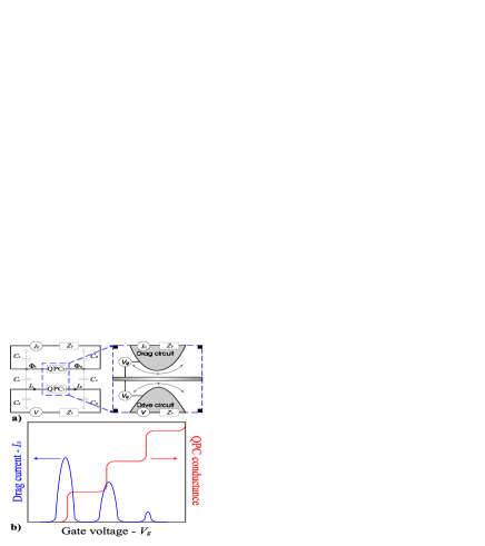
Figure 1: (Color online) a) Two coupled QPCs and surrounding electric circuitry. The Coulomb coupling is due to mutual capacitances $C_{c}$. Gate voltage $V_{g}$ control transmission of e.g. drive QPC. b) Schematic representation of linear conductance of the drive QPC along with the drag current as a function of the gate voltage.

Mesoscopic and quantum circuits with the spatial dimensions less than the temperature length $L_{T}=v_{F}/T$ and voltage length $L_{V}=v_{F}/eV$ differ from the bulk 2D systems in several important ways. (i) The electron-hole symmetry in such devices is broken much stronger than in bulk systems. In mesoscopic devices this is due to a random configurations of impurities Aleiner , while in the QPC’s the effect is due to the energy dependence of transmission coefficients. Because of the latter the hole’s transmission probability is typically less than that of the electrons. (ii) The spatial inversion symmetry may be broken by left-right asymmetry of the circuit design. As we show below, this makes two polarities of the drive voltage $V$ to be essentially non-equivalent. (iii) Because of the above, the quantum circuits may be easily driven out of the linear response domain (unlike the bulk systems). Typically a voltage needed to drive a quantum circuit into a nonlinear regime is parametrically smaller than the temperature.

In this paper we study drag effect between two QPC’s, Fig. 1a. We assume weak interaction between the two circuits mediated by mutual capacitances $C_{c}$, Fig. 1a. Since the external circuits typically include also dissipative elements, the actual interaction is, in general, frequency-dependent Aguado and determined by a matrix of trans-impedances (see below). Because of the weak coupling the drag current $I_{D}$ is small and therefore the drag circuit is assumed to be close to equilibrium. On the other hand, the drive circuit may be substantially out-of-equilibrium, due to an applied bias $V$. With these assumption we evaluate the drag current $I_{D}$ in the second-order in the inter-circuit interactions in the framework of the Keldysh diagrammatic technique (to account for non-equilibrium conditions of the drive circuit). Details of the calculations are reported as a supplementary material.

We show that at sufficiently small driving voltage $V$ the drag current is linear $I_{D}\propto V$. In this regime the mechanism of the drag is similar to that in the bulk 2D systems: i.e. rectification of near-equilibrium thermal noise. Consequently $I_{D}\propto T^{2}$ at small temperatures. The rectification relies on the electron-hole asymmetry, which is due to energy dependence of the transmission probability in a given channel. The asymmetry is the strongest near an opening of a new conductance channel. Indeed, in this case thermally excited electrons are much more likely to be transmitted than the holes. Hence the behavior sketched in Fig. 1b (though with no relation to the quantum shot noise). At larger drive voltages $I_{D}\propto V^{2}$ and the effect is indeed due to the detection of the excess shot noise of the drive circuit Kouwenhoven ; Khrapai ; Aguado ; Chudnovskiy . The energy dependence of the transmission probability is not required in this regime, and $I_{D}$ is proportional to the celebrated Fano factor Lesovik ; Reznikov ; BB . Remarkably, the crossover between the two regimes takes place at $eV\sim T^{2}/\Delta\ll T$, where $\Delta$ is an energy scale of the transmission probability.

Quantitatively we found the following expression for the drag current:

$$I_{D}(V)=\int\!\frac{d\omega}{4\pi\omega^{2}}\mathrm{Tr}\left[\hat{\mathcal{Z}}(\omega)\hat{S}_{1}(\omega,V)\hat{\mathcal{Z}}(-\omega)\hat{\Gamma}_{2}(\omega)\right]\,.$$ (1)

Here and throughout the paper indexes $1,2$ refer to the drive and drag circuits, correspondingly. The elements $\mathcal{Z}_{ab}(\omega)$, $a,b=R,L$ of the trans-impedance matrix $\hat{\mathcal{Z}}(\omega)$ encode inter-circuit coupling. They are defined as $\mathcal{Z}_{ab}(\omega)=\partial\Phi_{a}(\omega)/\partial I_{b}(\omega)$, where the corresponding local fluctuating currents $I_{a}$ and voltages $\Phi_{a}$ are indicated in Fig. 1a.

In Eq. (1) the drive circuit is characterized by the excess part $S^{ab}_{1}(\omega,V)=S_{ab}(\omega,V)-S_{ab}(\omega,0)$ of current-current correlation matrix $S_{ab}(\omega,V)=\int dt\,e^{i\omega t}\big{\langle}\big{\langle}\delta\hat{I}_{a}(t)\delta\hat{I}_{b}(0)+\delta\hat{I}_{b}(0)\delta\hat{I}_{a}(t)\big{\rangle}\big{\rangle}$, which is known from the theory of quantum shot noise Lesovik ; Buttiker ; BB-review . In particular

$$\hskip-14.22636ptS_{LL}(\omega,V)=\frac{2}{R_{Q}}\sum_{n}\int d\epsilon\left[B_{RR}(\epsilon)|\mathbf{t}^{R}_{n}(\epsilon_{+})|^{2}|\mathbf{t}^{R}_{n}(\epsilon_{-})|^{2}\right.$$

$$\hskip-14.22636pt+B_{LL}(\epsilon)\big{[}1-\mathbf{r}^{*L}_{n}(\epsilon_{+})\mathbf{r}^{L}_{n}(\epsilon_{-})\big{]}\big{[}1-\mathbf{r}^{*L}_{n}(\epsilon_{-})\mathbf{r}^{L}_{n}(\epsilon_{+})\big{]}$$

$$\hskip-14.22636pt+\left.B_{LR}(\epsilon)|\mathbf{r}^{L}_{n}(\epsilon_{+})|^{2}|\mathbf{t}^{R}_{n}(\epsilon_{-})|^{2}+B_{RL}(\epsilon)|\mathbf{t}^{R}_{n}(\epsilon_{+})|^{2}|\mathbf{r}^{L}_{n}(\epsilon_{-})|^{2}\right]\,,$$ (2)

with the similar expressions for $S_{LR}$, $S_{RL}$ and $S_{RR}$ components, see Ref. Buttiker and supplementary materials for details. Here $R_{Q}={2\pi\hbar\over e^{2}}$ is quantum resistance, $|\mathbf{t}^{L(R)}_{n}(\epsilon)|^{2}=|\mathbf{t}_{n}(\epsilon+eV_{L(R)})|^{2}$ are transmission probabilities of the drive QPC₁, labeled by the transverse channel index $n$; $|\mathbf{r}^{L(R)}_{n}(\epsilon)|^{2}=1-|\mathbf{t}^{L(R)}_{n}(\epsilon)|^{2}$ and $V_{L}-V_{R}=V$. The statistical factors are $B_{ab}(\epsilon)=f_{a}(\epsilon_{+})[1-f_{b}(\epsilon_{-})]+f_{b}(\epsilon_{-})[1-f_{a}(\epsilon_{+})]$, with $f_{L(R)}(\epsilon)=f(\epsilon+eV_{L(R)})$ being the Fermi distributions of the two leads and $\epsilon_{\pm}=\epsilon\pm\omega/2$.

The drag circuit in Eq. (1) is characterized by the rectification coefficient $\hat{\Gamma}_{2}(\omega)=\Gamma_{2}(\omega)\hat{\tau}_{z}$ of the ac voltage fluctuations applied to the (near equilibrium) drag QPC₂, where $\hat{\tau}_{z}$ is third Pauli matrix acting in the left-right space. Rectification is given by

$$\Gamma_{2}(\omega)=\frac{2e}{R_{Q}}\sum_{n}\int\!d\epsilon\,\big{[}f(\epsilon_{-})-f(\epsilon_{+})\big{]}\Big{[}|\mathbf{t}_{n}(\epsilon_{+})|^{2}-|\mathbf{t}_{n}(\epsilon_{-})|^{2}\Big{]}\,.$$ (3)

Characteristics of the QPC₂ enter through its energy-dependent transmission probabilities $|\mathbf{t}_{n}(\epsilon)|^{2}$. This expression admits a transparent interpretation: potential fluctuations with frequency $\omega$, say on the left of the QPC, create electron-hole pairs with energies $\epsilon_{\pm}$ on the branch of right moving particles. Consequently the electrons can pass through the QPC with the probability $|\mathbf{t}_{n}(\epsilon_{+})|^{2}$, while the holes with the probability $|\mathbf{t}_{n}(\epsilon_{-})|^{2}$. The difference between the two gives the dc current flowing across the QPC. Notice that the energy dependence of the transmission probabilities in the drag QPC is crucial Footnote-2 in order to have the asymmetry between electrons and holes, and thus non-zero rectification $\Gamma_{2}(\omega)$.

Focusing on a single partially open channel in a smooth QPC, one may think of the potential barrier across it as being practically parabolic. In such a case its transmission probability is given by

$$|\mathbf{t}(\epsilon)|^{2}=\left(\exp\{(eV_{g}-\epsilon)/\Delta_{2}\}+1\right)^{-1}\,,$$ (4)

where $\Delta_{2}$ is an energy scale associated with the curvature of the parabolic barrier in the QPC₂ and gate voltage $V_{g}$ moves the top of the barrier relative to the Fermi energy. This form of transmission was used to explain QPC conductance quantization Glazman and it turns out to be useful in application to the Coulomb drag problem. Inserting (4) into (3) and carrying out energy integration, one finds

$$\Gamma_{2}(\omega)=\frac{2e\Delta_{2}}{R_{Q}}\,\ln\left(1+\frac{\sinh^{2}(\omega/2\Delta_{2})}{\cosh^{2}(eV_{g}/2\Delta_{2})}\right)$$ (5)

for $T\ll\Delta_{2}$. In the other limit, $T\gg\Delta_{2}$, one should replace $\Delta_{2}\to T$ in the Eq. (5). Notice that for small frequency $\omega\ll\Delta_{2}$ one has $\Gamma_{2}\sim\omega^{2}$, making the the integral in Eq. (1) to be convergent in $\omega\to 0$ region.

Linear drag regime. For small applied voltages $V$ one expects the response current $I_{D}$ to be linear in $V$. Expanding $\hat{S}_{1}(\omega,V)$ to the linear order in $V$, one finds that only diagonal components of the current-current correlation matrix contribute to the linear response and as a result

$$\hat{S}_{1}(\omega,V)=V\,\frac{\partial}{\partial\omega}\left[\coth\frac{\omega}{2T}\right]\hat{\Gamma}_{1}(\omega)+O(V^{3})\,,$$ (6)

where $\Gamma_{1}(\omega)$ is obtained from Eq. (3) by substituting transmission probabilities of QPC₂, by that of QPC₁. Inserting Eq. (6) into Eq. (1) one finds

$$I_{D}=V\,\frac{R^{2}_{Q}}{4\pi}\int\!d\omega\,\frac{\alpha_{+}(\omega)}{\omega^{2}}\,\frac{\partial}{\partial\omega}\left[\coth\frac{\omega}{2T}\right]\Gamma_{1}(\omega)\,\Gamma_{2}(\omega)\,,$$ (7)

where dimensionless interaction kernel $\alpha_{+}(\omega)$ is expressed through the components of the trans-impedance matrix as $\alpha_{\pm}(\omega)=\big{[}\big{(}|\mathcal{Z}_{LL}|^{2}-\mathcal{Z}_{LR}\mathcal{Z}_{RL}\big{)}\pm\big{(}|\mathcal{Z}_{RR}|^{2}-\mathcal{Z}_{LR}\mathcal{Z}_{RL}\big{)}\big{]}/2R^{2}_{Q}$. Derived equation (7) has the same general structure as the one for the drag current in bulk 2D systems Kamenev-Oreg ; Flensberg . Being symmetric with respect $1\leftrightarrow 2$ permutation, it satisfies Onsager relation for the linear response coefficient.

Assuming the load impedance of the drag circuit to be much larger than that of the drive one $Z_{1}\ll Z_{2}\ll R_{Q}$ and the mutual capacitance of the two circuits to be small $C_{c}\ll C_{R,L,s}$, see Fig. 1a, one finds for the low frequency limit $\omega\ll(Z_{1}C_{s})^{-1}$ of the interaction kernels

$$\alpha_{\pm}(0)=\frac{Z^{2}_{1}}{8R_{Q}^{2}}\,\frac{C_{c}^{2}}{C_{L}^{2}C_{R}^{2}}\times\left\{\begin{array}[]{l}2C_{L}^{2}+2C_{L}C_{R}+2C_{R}^{2}\\ C_{L}^{2}-C_{R}^{2}\end{array}\right.\,.$$ (8)

For $Z_{1}\to 0$ the drive QPC is shorted and the drag circuit is insensitive to the fluctuations. Substituting now Eq. (5) into Eq. (7), one finds for e.g. low-temperature regime $T\ll\Delta_{1,2}$

$$I_{D}=\frac{V}{R_{Q}}\,\frac{\alpha_{+}(0)\pi^{2}}{6}\,{T^{2}\over\Delta_{1}\Delta_{2}}\,{1\over\cosh^{2}(eV_{g}/2\Delta_{1})}\,,$$ (9)

where we assumed that the gate voltage of QPC₂ is tuned to adjust the top of its barrier with the Fermi energy and wrote $I_{D}$ as a function of the gate voltage in QPC₁. We have also assumed that $T\ll(Z_{1}C_{s})^{-1}$ to substitute $\alpha_{+}(\omega)$ by its dc limit Eq. (8). The resulting expression exhibits a peak at $V_{g}=0$ similar to that depicted in Fig. 1b. Yet it has nothing to do with the shot noise, but rather reflects rectification of near-equilibrium thermal fluctuations (hence the factor $T^{2}$) along with the electron-hole asymmetry (hence non-monotonous dependence on $V_{g}$). For monotonously increasing functions $|\mathbf{t}(\epsilon)|^{2}$ in both circuits the linear drag is positive (i.e. currents flow in the same direction).

Nonlinear regime. At larger drive voltages drag current ceases to be linear in $V$. Furthermore, contrary to the linear response case, $\hat{S}_{1}(\omega,V)$ does not require energy dependence of the transmission probabilities and could be evaluated for energy independent $|\mathbf{t}_{n}|^{2}$ (this is a fare assumption for $T,eV\ll\Delta_{1}$). Assuming in addition $T\ll eV$, one finds a celebrated expression for the quantum shot noise Lesovik ; BB-review

$$\hat{S}_{1}(\omega,V)=2\frac{|eV+\omega|+|eV-\omega|}{R_{Q}}\sum_{n}|\mathbf{t}_{n}|^{2}\Big{[}1-|\mathbf{t}_{n}|^{2}\Big{]}\hat{\tau}_{0}\,.$$ (10)

Inserting Eq. (10) into Eq. (1), after frequency integration bounded by the voltage, one finds for the drag current Footnote-3

$$I_{D}=\frac{eV^{2}}{\Delta_{2}R_{Q}}\,\alpha_{-}(0)\,\sum_{n}|\mathbf{t}_{n}|^{2}\Big{[}1-|\mathbf{t}_{n}|^{2}\Big{]}\,.$$ (11)

Here again we assumed that the detector QPC₁ is tuned to the transition between the plateaus. We also assumed $eV\ll(Z_{1}C_{s})^{-1}$ to substitute $\alpha_{-}(\omega)$ by its dc value, Eq. (8). One should notice that while $\alpha_{+}>0$, the sign of $\alpha_{-}$ is arbitrary. For a completely symmetric circuit $\alpha_{-}=0$, while for extremely asymmetric one $|\alpha_{-}|\lesssim\alpha_{+}/2$. Although we presented derivation of Eq. (11) for $T\ll eV$, one may show that it remains valid at any temperature as long as $T\ll\mathrm{min}\{\Delta_{1},(Z_{1}C_{s})^{-1}\}$.

Equation (11) indeed shows that the drag current is due to the rectification of the quantum shot noise and hence proportional to the Fano factor Lesovik . It again exhibits a generic behavior depicted in Fig. 1b, but the reason is rather different from the similar behavior in the linear regime. The direction of the nonlinear drag current is determined by the inversion asymmetry of the circuit (through the sign of $\alpha_{-}$) rather than the direction of the drive current. As a result, for a certain polarity of the drive voltage, the drag current appears to be negative.

We discuss now a crossover between the two regimes. Assuming that for a generic circuit $\alpha_{+}\sim\alpha_{-}$ and comparing Eqs. (9) and (11) one concludes that the transition from the linear to the nonlinear regime takes place at $V\approx V^{*}$ with

$$eV^{*}=T^{2}/\Delta_{1}\ll T\,,$$ (12)

for $T\ll\Delta_{1}$. In the opposite limit, $T>\Delta_{1}$, the crossover voltage is given by the temperature $eV^{*}=T$. However, for a circuit with an almost perfect inversion symmetry, i.e. $\alpha_{-}\ll\alpha_{+}$, the nonlinear regime may be pushed to substantially larger voltages. Such a symmetric circuitry is not well suited for detection of the quantum shot noise.

Mesoscopic circuits. One or both circuits may be represented by a multichannel quasi-1D (or 2D) mesoscopic sample. In this case $\sum_{n}|\mathbf{t}_{n}(\epsilon)|^{2}=g(\epsilon)$ is a dimensionless (in units of $R_{Q}^{-1}$) conductance of the sample as a function of its Fermi energy. Such a conductance exhibits universal conductance fluctuations (UCF) UCF , that is $g(\epsilon)=g+\delta g(\epsilon)$, where $g\gg 1$ is an average conductance and $\delta g(\epsilon)\sim 1$ is a sample and energy-dependent fluctuating part. The characteristic scale of the energy dependence of the fluctuating part is the Thouless energy $E_{Th}=\hbar D/L^{2}$, where $D$ is electronic diffusion constant and $L$ is the sample size. Employing Eq. (3), one finds that the rectification coefficient of a given mesoscopic sample may be estimated as

$$\Gamma(\omega)\sim\pm{e\over R_{Q}}\,\frac{\omega^{2}}{E_{Th}}\,,\quad\quad\{T,\omega\}\ll E_{Th}\,.$$ (13)

On the other hand, the nonequilibrium part of the noise correlator Eq. (10) exhibits a well-defined average value

$$S_{1}(\omega,V)=2\left(|eV+\omega|+|eV-\omega|\right){g\over 3R_{Q}}\,,$$ (14)

the coefficient $1/3$ is specific to a quasi-1D geometry BB .

In the Coulomb drag setup, where both circuits are represented by mesoscopic elements, employing Eqs. (1), (7) along with (13), (14), one finds for the drag current (both linear and nonlinear)

$$I_{D}\sim\frac{V}{R_{Q}}\,\left(\alpha_{+}\,{T^{2}\over E_{Th}^{2}}\,+\,\alpha_{-}\,{eV\over E_{Th}}\,g\right)\,,$$ (15)

where $T<E_{Th}$. If the load impedance of the drive circuit is $Z_{1}\sim g^{-1}$, then linear in $V$ term of Eq. (15) is in agreement with the corresponding result of Ref. Aleiner . The crossover between linear and nonlinear regimes takes place at $eV^{*}=\alpha_{+}T^{2}/(\alpha_{-}gE_{Th})$ which may be much less than both $T$ and $E_{Th}$. As a result, one may expect drag current to be substantially bigger than the linear response prediction already at the very modest bias voltage.

In summary, we have studied Coulomb drag effect in the system of two coupled quantum circuits. In the linear regime gate voltage induced oscillations of the drag conductance originate from the particle-hole asymmetry, which is encoded in the energy dependent transmission probabilities of the QPC. The drag conductance follows quadratic temperature dependence at low temperatures and is peaked at gate voltages, which correspond to the transition between QPC conductance plateaus. Beyond the linear regime the magnitude of the drag current is proportional to the current shot noise generated in the drive QPC.

We are grateful to A. Chudnovskiy, L. Glazman, F. von-Oppen, and B. Shklovskii for useful discussions. We are indebted to M. Büttiker for pointing out on error in a previous version of Eq. (Coulomb drag in quantum circuits). This work was supported by NSF grants DMR-0405212 and DMR-0804266.

Supplementary materials

The purpose of this section is to provide technical details needed to derive Eq. (1) of the main paper. To this end, we describe each point contact of the quantum circuit Fig. 1a as quasi-1D adiabatic constriction connected to two reservoirs (terminals, probes), to be referred to as left ($L$) and right ($R$). The distribution functions of electrons in the reservoirs of a driven circuit, are Fermi distributions $f_{L(R)}(\epsilon)=\big{[}\exp[(\epsilon+eV_{L(R)})/T]+1\big{]}^{-1}$, with source-drain voltage being $V_{L}-V_{R}=V$. In the dragged circuit distributions are assumed to be equilibrium Fermi functions. Within each QPC electron motion is separable into transverse and longitudinal components. Due to the confinement transverse motion is quantized and we assign quantum number $n$ to label transverse conduction channels with $\phi_{n}(r_{\perp})$ being corresponding transversal wave function. The longitudinal motion is describe in terms of the extended scattering states – normalized electron plane waves incident from the left

$$u^{L}_{n}(k,r)=\frac{\phi_{n}(r_{\perp})}{\sqrt{v}}\left\{\begin{array}[]{cc}e^{ikx}+\mathbf{r}_{n}(k)e^{-ikx}&x\to-\infty\\ \mathbf{t}_{n}(k)e^{ikx}&x\to+\infty\end{array}\right.$$ (16)

and right

$$u^{R}_{n}(k,r)=\frac{\phi_{n}(r_{\perp})}{\sqrt{v}}\left\{\begin{array}[]{cc}e^{-ikx}+\mathbf{r}_{n}(k)e^{ikx}&x\to+\infty\\ \mathbf{t}_{n}(k)e^{-ikx}&x\to-\infty\end{array}\right.$$ (17)

onto mesoscopic scattering region. Here $k$ and $v$ are the electron wave vector and velocity, $\mathbf{t}_{n}(k)$ and $\mathbf{r}_{n}(k)$ are channel specific transmission and reflection amplitudes. Second quantized electron field operator is introduced in the standard way

$$\hat{\Psi}(r,t)=\sum_{nk}\left[\hat{\psi}^{L}_{n}(k,t)u^{L}_{n}(k,r)+\hat{\psi}^{R}_{n}(k,t)u^{R}_{n}(k,r)\right]\,,$$ (18)

where $\hat{\psi}^{L(R)}_{n}(k,t)$ are fermion destruction operators in the left and right reservoirs correspondingly. For the future use we define also current operator

$$\hat{I}_{a}(t)=\sum_{nk}M^{a}_{nn^{\prime}}\hat{\psi}^{{\dagger}a}_{n}(k,t)\hat{\psi}^{a}_{n^{\prime}}(k^{\prime},t)\,,$$ (19)

which has matrix elements $M^{a}_{nn^{\prime}}=(e/2im)\int dr_{\perp}\big{[}u^{*a}_{n}(k,r)\partial_{x}u^{a}_{n^{\prime}}(k^{\prime},r)-\partial_{x}[u^{*a}_{n}(k,r)]u^{a}_{n^{\prime}}(k^{\prime},r)\big{]}$, constructed from the scattering states (16)–(17). Based on the orthogonality condition of transverse wave functions $\int dr_{\perp}\phi^{\phantom{*}}_{n}(r_{\perp})\phi^{*}_{n^{\prime}}(r_{\perp})=\delta_{nn^{\prime}}$, direct calculation gives

$$M^{L}_{nn^{\prime}}=-e\delta_{nn^{\prime}}\left(\begin{array}[]{ll}\mathbf{r}^{*}_{n}(k)\mathbf{r}_{n}(k^{\prime})-1&\mathbf{r}^{*}_{n}(k)\mathbf{t}_{n}(k^{\prime})\\ \mathbf{t}^{*}_{n}(k)\mathbf{r}_{n}(k^{\prime})&\mathbf{t}^{*}_{n}(k)\mathbf{t}_{n}(k^{\prime})\end{array}\right)\,,$$ (20)

and a similar result for $M^{R}_{nn^{\prime}}$. In Eq. (20) we have suppressed phase factors $e^{\pm i(k-k^{\prime})x}\approx 1$, since $|k-k^{\prime}|\sim L_{T}^{-1}\ll x^{-1}$, and the coordinate $x$ is confined by the sample size $L\ll L_{T}$. On the other hand, we do not keep fast oscillating factors $e^{\pm 2ik_{F}x}$, since $x\sim L\gg k_{F}^{-1}$. However, one must keep explicitly momentum (or equivalently energy) dependence for transmission amplitudes, which translates later into particle–hole asymmetry factor $\Gamma(\omega)$.

Dynamics of $\hat{\psi}^{L(R)}_{n}(k,t)$ operators is governed by the action

$$i\mathcal{S}_{0}=\int_{C}dt\sum_{ja}\sum_{nk}\bar{\psi}^{a}_{jn}(k,t)i\hat{\mathbf{G}}^{-1}\psi^{a}_{jn}(k,t)$$ (21)

defined along the Keldysh contour, where $\hat{\mathbf{G}}^{-1}=(i\partial_{t}-\xi_{k}+eV_{a})$ is Green’s function operator with $\xi_{k}$ being electron energy. Additional subscript $j$ in Eq. (21) labels drive $(j=1)$ and drag $(j=2)$ QPC’s. As usual for Keldysh technique one splits time integration into forward and backward pathes and replicates each fermion field into two components $\psi\Rightarrow\psi^{\rightleftarrows}$, which belong now to the different contour branches. It is convenient also to perform Keldysh rotation

$$\left(\begin{array}[]{c}\psi^{+}\\ \psi^{-}\end{array}\right)=\hat{\mathbb{L}}\hat{\sigma}_{z}\left(\begin{array}[]{c}\psi^{\rightarrow}\\ \psi^{\leftarrow}\end{array}\right),\,\left(\begin{array}[]{c}\bar{\psi}^{+}\\ \bar{\psi}^{-}\end{array}\right)=\hat{\mathbb{L}}\left(\begin{array}[]{c}\bar{\psi}^{\rightarrow}\\ \bar{\psi}^{\leftarrow}\end{array}\right)\,,\hat{\mathbb{L}}=\frac{1}{\sqrt{2}}\left(\begin{array}[]{cc}1&-1\\ 1&\phantom{-}1\end{array}\right),$$ (22)

where $\hat{\sigma}_{z}$ is third Pauli matrix acting in the Keldysh space. In this rotated basis quadratic action (21) gives following electron correlators

$$-i\langle\langle\psi^{a\alpha}_{in}(k,t)\bar{\psi}^{b\beta}_{jn}(k,t^{\prime})\rangle\rangle=\delta_{ij}\delta_{ab}\mathbf{G}^{\alpha\beta}_{ia}(t,t^{\prime})\,,$$ (23)

where Keldysh Green’s function matrix has familiar triangular structure

$$\mathbf{G}^{\alpha\beta}_{ia}(t,t^{\prime})=\left(\begin{array}[]{cc}G^{R}_{ia}(t,t^{\prime})&G^{K}_{ia}(t,t^{\prime})\\ 0&G^{A}_{ia}(t,t^{\prime})\end{array}\right)^{\alpha\beta}.$$ (24)

Retarded/Advanced/Keldysh components of $\mathbf{G}^{\alpha\beta}$ are given by

$$iG^{R}_{ia}(t,t^{\prime})=\theta(t-t^{\prime})e^{-i(\xi_{k}+eV_{a})(t-t^{\prime})}\,,$$

$$iG^{A}_{ia}(t,t^{\prime})=-\theta(t^{\prime}-t)e^{-i(\xi_{k}+eV_{a})(t-t^{\prime})}\,,$$ (25)

$$iG^{K}_{ia}(t,t^{\prime})=[1-2f_{a}(\epsilon_{k})]e^{-i(\xi_{k}+eV_{a})(t-t^{\prime})}\,.$$

Having described quantum point contacts individually we introduce now the interaction term between them

$$i\mathcal{S}_{\mathrm{int}}=\sum_{ab\alpha\beta}\iint^{+\infty}_{-\infty}dtdt^{\prime}\,I^{\alpha}_{1a}(t)\mathbf{K}^{\alpha\beta}_{ab}(t-t^{\prime})I^{\beta}_{2b}(t^{\prime})\,.$$ (26)

Here $I_{jR(L)}(t)$ are current operators (19), on the right (left) of the QPC_j, coupled by the kernel $\mathbf{K}(t-t^{\prime})$, which encodes electromagnetic environment of the circuit. Interaction kernel retarded and advanced components are directly related to the trans-impedance matrix of the circuit $\mathbf{K}^{R(A)}_{ab}(\omega)=\mathcal{Z}^{R(A)}_{ab}(\omega)/(\omega\pm i0)$, while Keldysh component can be restored from the fluctuation-dissipation theorem: $\mathbf{K}^{K}_{ab}(\omega)=[\mathbf{K}^{R}_{ab}(\omega)-\mathbf{K}^{A}_{ab}(\omega)]\coth(\omega/2T)$, i.e. we assume the surrounding electric environment to be close to equilibrium.

Figure 2: Drag current $I_{D}$ in the second order in inter-circuit interactions $\mathbf{K}=\mathcal{Z}/\omega$ (wavy lines). The drag circuit is represented by triangular rectification vertex $\Gamma_{2}(\omega)$, while the drive circuit by the non-equilibrium current-current correlator $S_{1}(\omega,V)$ (loop).

Within this formalism, drag current is found by averaging $I_{2}$ over the fermionic degrees of freedom

$$I_{D}=\int\mathbf{D}[\psi\bar{\psi}]\,\mathrm{Tr}\left[\bar{\psi}_{2}M\psi_{2}\right]\,\exp\big{(}i\mathcal{S}[\bar{\psi}\psi]\big{)}\,,$$ (27)

where $\mathcal{S}=\mathcal{S}_{0}+\mathcal{S}_{\mathrm{int}}$ and we used expression (19) for the current operator. Being interested in the leading perturbative result, we expand $\exp(i\mathcal{S})$ to the second order in interaction term $\mathcal{S}_{\mathrm{int}}$. This way one obtains

$$\!\!\!\!\!I_{D}=\frac{1}{2}\int\mathbf{D}[\psi\bar{\psi}]\!\!\!\!\! \mathrm{Tr}\left[\bar{\psi}_{2}M\psi_{2}\right]$$ (28)

$$\mathrm{Tr}\left[I_{1}\mathbf{K}I_{2}\right]\mathrm{Tr}\left[I_{1}\mathbf{K}I_{2}\right]\exp\big{(}i\mathcal{S}_{0}[\bar{\psi}\psi]\big{)}.$$

Remaining Gaussian integral may be evaluating using the Wick’s theorem. One inserts expressions (19) for the current operators into the traces of (28) and takes into the account all the possible Wick’s contraction between $\psi$-fields. The latter are given by the Green’s functions (23). This way we find our main result for the drag current [Eq. (1)] shown diagrammatically in the Fig. 2. The interaction kernels $\alpha_{\pm}(\omega)$, rectification coefficient $\Gamma_{2}(\omega)$ and noise power $S_{ab}(\omega,V)$ are given explicitly by the following Keldysh traces:

$$\alpha_{+(-)}(\omega)=\frac{1}{2R^{2}_{Q}}\mathrm{Tr}\left[\hat{\mathcal{Z}}^{R}(\omega)\hat{\tau}_{0(z)}\hat{\mathcal{Z}}^{A}(\omega)\tau_{z}\right]\,,$$ (29)

$$S_{ab}(\omega,V)=\mathrm{Tr}\left[\hat{\mathbf{G}}\hat{\sigma}_{x}\hat{M}_{a}\hat{\mathbf{G}}\hat{\sigma}_{x}\hat{M}_{b}\right]\,,$$ (30)

$$\Gamma_{2}(\omega)=\mathrm{Tr}\left[\hat{\mathbf{G}}\hat{\sigma}_{x}\hat{M}\hat{\mathbf{G}}\hat{\sigma}_{0}\hat{M}\hat{\mathbf{G}}\hat{\sigma}_{0}\hat{M}\right]\,,$$ (31)

where $\hat{\tau}$ and $\hat{\sigma}$ are two sets of Pauli matrices in left-right and Keldysh spaces, correspondingly.

Remaining steps of algebra concern calculation of the traces in Eqs. (29)–(31). For the interaction coefficients $\alpha_{\pm}$ it is straightforward. Let us demonstrate how Eq. (2) for $S_{LL}$ is recovered from Eq. (30). To this end we insert current matrix $M^{L}$ [Eq. (20)] along with $\hat{\mathbf{G}}=\mathrm{diag}\{\hat{G}_{L},\hat{G}_{R}\}$ into Eq. (30) and calculate trace over left-right subspace, which gives

$$\hskip-5.69046ptS_{LL}(\omega,V)=e^{2}\sum_{n}\int\frac{d\epsilon}{2\pi}\int\frac{d\xi d\xi^{\prime}}{4\pi^{2}}$$ (32)

$$\hskip-5.69046pt\left[\mathrm{Tr}\big{[}\hat{G}_{L}(\epsilon_{+},\xi)\hat{\sigma}_{x}\hat{G}_{L}(\epsilon_{-},\xi^{\prime})\hat{\sigma}_{x}\big{]}[\mathbf{r}^{*}_{n}(\xi)\mathbf{r}_{n}(\xi^{\prime})-1][\mathbf{r}^{*}_{n}(\xi^{\prime})\mathbf{r}_{n}(\xi)-1]\right.$$

$$\hskip-5.69046pt+\mathrm{Tr}\big{[}\hat{G}_{L}(\epsilon_{+},\xi)\hat{\sigma}_{x}\hat{G}_{R}(\epsilon_{-},\xi^{\prime})\hat{\sigma}_{x}\big{]}|\mathbf{r}_{n}(\xi)|^{2}|\mathbf{t}_{n}(\xi^{\prime})|^{2}$$

$$\hskip-5.69046pt+\mathrm{Tr}\big{[}\hat{G}_{R}(\epsilon_{+},\xi)\hat{\sigma}_{x}\hat{G}_{L}(\epsilon_{-},\xi^{\prime})\hat{\sigma}_{x}\big{]}|\mathbf{t}_{n}(\xi)|^{2}|\mathbf{r}_{n}(\xi^{\prime})|^{2}$$

$$\hskip-5.69046pt\left.+\mathrm{Tr}\big{[}\hat{G}_{R}(\epsilon_{+},\xi)\hat{\sigma}_{x}\hat{G}_{R}(\epsilon_{-},\xi^{\prime})\hat{\sigma}_{x}\big{]}|\mathbf{t}_{n}(\xi)|^{2}|\mathbf{t}_{n}(\xi^{\prime})|^{2}\right]\,.$$

Recall here that $\hat{G}_{L(R)}$ are still matrices in the Keldysh subspace. Using Eq. (24) one calculates remaining traces over the Keldysh subspace

$$\mathrm{Tr}\left[\hat{G}_{a}\hat{\sigma}_{x}\hat{G}_{b}\hat{\sigma}_{x}\right]=G^{R}_{a}G^{A}_{b}+G^{A}_{a}G^{R}_{b}+G^{K}_{a}G^{K}_{b}\,,$$ (33)

and performs final integration with the help of Green’s functions $G^{R(A)}_{a}(\epsilon,\xi)=(\epsilon-\xi+eV_{a}\pm i0)^{-1}$ and $G^{K}_{a}(\epsilon,\xi)=-2\pi i\delta(\epsilon-\xi+eV_{a})\big{[}1-2f_{a}(\xi)\big{]}$, which follows from Fourier transforms of Eq. (Supplementary materials). It is not difficult to see now that each Keldysh trace in Eq. (32) defines statistical occupation factors $B_{ab}(\epsilon)$ used in Eq. (2), namely $\mathrm{Tr}\left[\hat{G}_{a}\hat{\sigma}_{x}\hat{G}_{b}\hat{\sigma}_{x}\right]\propto B_{ab}(\epsilon)$. As a result, collecting all the factors, one finds from Eq. (33) the final form of noise power given by Eq. (2). In complete analogy one may calculate $S_{RR}$ and $S_{LR}$ components of the noise power:

$$\hskip-14.22636ptS_{RR}(\omega,V)=\frac{2}{R_{Q}}\sum_{n}\int d\epsilon\left[B_{LL}(\epsilon)|\mathbf{t}^{L}_{n}(\epsilon_{+})|^{2}|\mathbf{t}^{L}_{n}(\epsilon_{-})|^{2}\right.$$ (34)

$$\hskip-14.22636pt+B_{RR}(\epsilon)\big{[}1-\mathbf{r}^{*R}_{n}(\epsilon_{+})\mathbf{r}^{R}_{n}(\epsilon_{-})\big{]}\big{[}\mathbf{r}^{*R}_{n}(\epsilon_{-})\mathbf{r}^{R}_{n}(\epsilon_{+})-1\big{]}$$

$$\hskip-14.22636pt\left.+B_{LR}(\epsilon)|\mathbf{t}^{L}_{n}(\epsilon_{+})|^{2}|\mathbf{r}^{R}_{n}(\epsilon_{-})|^{2}+B_{RL}(\epsilon)|\mathbf{r}^{R}_{n}(\epsilon_{+})|^{2}|\mathbf{t}^{L}_{n}(\epsilon_{-})|^{2}\right]\,,$$

$$\hskip-14.22636ptS_{LR}(\omega,V)=-\frac{2}{R_{Q}}\sum_{n}\int d\epsilon$$ (35)

$$\hskip-14.22636pt\left[B_{LL}(\epsilon)\big{[}\mathbf{t}^{*L}_{n}(\epsilon_{+})\mathbf{t}^{L}_{n}(\epsilon_{-})-\mathbf{t}^{*L}_{n}(\epsilon_{+})\mathbf{t}^{L}_{n}(\epsilon_{-})\mathbf{r}^{*L}_{n}(\epsilon_{-})\mathbf{r}^{L}_{n}(\epsilon_{+})\big{]}\right.$$

$$\hskip-14.22636pt+B_{RR}(\epsilon)\big{[}\mathbf{t}^{R}_{n}(\epsilon_{+})\mathbf{t}^{*R}_{n}(\epsilon_{-})-\mathbf{t}^{*R}_{n}(\epsilon_{+})\mathbf{t}^{R}_{n}(\epsilon_{-})\mathbf{r}^{R}_{n}(\epsilon_{+})\mathbf{r}^{*R}_{n}(\epsilon_{-})\big{]}$$

$$\hskip-14.22636pt+B_{LR}(\epsilon)\mathbf{t}^{*L}_{n}(\epsilon_{+})\mathbf{t}^{R}_{n}(\epsilon_{-})\mathbf{r}^{*R}_{n}(\epsilon_{-})\mathbf{r}^{L}_{n}(\epsilon_{+})$$

$$\hskip-14.22636pt\left.+B_{RL}(\epsilon)\mathbf{t}^{*R}_{n}(\epsilon_{+})\mathbf{t}^{L}_{n}(\epsilon_{-})\mathbf{r}^{*L}_{n}(\epsilon_{-})\mathbf{r}^{R}_{n}(\epsilon_{+})\right]\,.$$

Notice that cross-correlation component is negative.

Finding $\Gamma_{2}(\omega)$ one uses the fact that Green’s function is diagonal unity in the left-right subspace $\hat{\mathbf{G}}=\hat{G}\hat{\tau}_{0}$ and faces Keldysh trace of the kind

$$\mathrm{Tr}\left[\hat{G}\hat{\sigma}_{x}\hat{G}\hat{\sigma}_{0}\hat{G}\hat{\sigma}_{0}\right]=\sum_{\pm}\left[G^{R}(\epsilon)G^{R}(\epsilon\pm\omega)G^{K}(\epsilon)\right.$$

$$+\left.G^{R}(\epsilon)G^{K}(\epsilon\pm\omega)G^{A}(\epsilon)+G^{K}(\epsilon)G^{A}(\epsilon\pm\omega)G^{A}(\epsilon)\right].$$ (36)

To simplify this equation one should decompose each Keldysh component of the Green’s function using fluctuation-dissipation relation $G^{K}(\epsilon)=\big{[}G^{R}(\epsilon)-G^{A}(\epsilon)\big{]}[1-2f(\epsilon)]$ and keep in the resulting expression only those terms, which have different causality. Combinations having three Green’s functions of the same kind, like $G^{A}G^{A}G^{A}$ and $G^{R}G^{R}G^{R}$, will not contribute. This way, one finds that $\mathrm{Tr}\left[\hat{G}\hat{\sigma}_{x}\hat{G}\hat{\sigma}_{0}\hat{G}\hat{\sigma}_{0}\right]\propto\big{[}f(\epsilon_{-})-f(\epsilon_{+})\big{]}$, with $\epsilon_{\pm}=\epsilon\pm\omega/2$. Remaining trace over the current vertex matrices $M_{2}$ reduces to the transmission probabilities at shifted energies, namely $\mathrm{Tr}\big{[}M_{2}M_{2}M_{2}\big{]}\propto\pm|\mathbf{t}_{n}(\epsilon_{\pm})|^{2}$. As the result, imposing remaining $\epsilon$ integration and summation over transverse channels, one arrives at $\Gamma_{2}(\omega)$ in the form of Eq. (4) of the main text. This completes our derivation.

References

• (1) P.M. Solomon, P.J. Price, D.J. Frank, and D.C. La Tulipe, Phys. Rev. Lett. 63, 2508 (1989).
• (2) T.J. Gramila J. P. Eisenstein, A. H. MacDonald, L. N. Pfeiffer, and K. W. West, Phys. Rev. Lett. 66 1216 (1991).
• (3) U. Sivan, P.M. Solomon, and H. Shtrikman, Phys. Rev. Lett. 68, 1196 (1992).
• (4) M. P. Lilly, J. P. Eisenstein, L. N. Pfeiffer, and K. W. West, Phys. Rev. Lett. 80, 1714 (1998).
• (5) R. Pillarisetty, Hwayong Noh, D. C. Tsui, E. P. De Poortere, E. Tutuc, and M. Shayegan, Phys. Rev. Lett. 89, 016805 (2002).
• (6) A. S. Price, A. K. Savchenko, B. N. Narozhny, G. Allison, D. A. Ritchie, Science, 316, 99 (2007).
• (7) A.-P. Jauho and H. Smith, Phys. Rev. B 47, 4420 (1993).
• (8) L. Zheng and A.H. MacDonald, Phys. Rev. B 48, 8203 (1993).
• (9) A. Kamenev and Y. Oreg, Phys. Rev. B 52, 7516 (1995).
• (10) K. Flensberg, B.Y.-K. Hu, A.-P. Jauho and J. M. Kinaret, Phys. Rev. B 52, 14761 (1995).
• (11) P. Debray, P. Vasilopoulos, O. Raichev, R. Perrin, M. Rahman, and W. C. Mitchel, Physica E, 6, 694, (2000).
• (12) P. Debray, V. Zverev, O. Raichev, R. Klesse, P. Vasilopoulos, and R. S. Newrock, J. Phys.: Condens. Matter 13, 3389, (2001).
• (13) T. Morimoto, Y. Iwase, N. Aoki, T. Sasaki, Y. Ochiai, A. Shalios, J. P. Bird, M. P. Lilly, J. L. Reno, and J. A. Simmons, Appl. Phys. Lett. 82, 3952, (2003).
• (14) M. Yamamoto, M. Stopa, Y. Tokura, Y. Hirayama, and S. Tarucha, Science 313, 204, (2006).
• (15) R. Aguado and L. P. Kouwenhoven, Phys. Rev. Lett. 84, 1986 (2000).
• (16) E. Onac, F. Balestro, L. H. Willems van Beveren, U. Hartmann, Y. V. Nazarov, and L. P. Kouwenhoven, Phys. Rev. Lett. 96, 176601, (2006).
• (17) V. S. Khrapai, S. Ludwig, J. P. Kotthaus, H. P. Tranitz, and W. Wegscheider, Phys. Rev. Lett. 97, 176803 (2006) and Phys. Rev. Lett. 99, 096803, (2007).
• (18) A. L. Chudnovskiy, preprint arXiv[cond-mat]:0710.2403.
• (19) G. B. Lesovik, JETP Lett. 49, 592 (1989).
• (20) M. Reznikov, M. Heiblum, Hadas Shtrikman, and D. Mahalu, Phys. Rev. Lett. 75, 3340 (1995).
• (21) This is the case in the lowest (second) order in inter-circuit interactions. In higher orders in interactions drag conductance may be temperature independent, see Ref. LK .
• (22) A. Levchenko and A. Kamenev, Phys. Rev. Lett. 100, 026805 (2008).
• (23) B. N. Narozhny and I. L. Aleiner, Phys. Rev. Lett. 84, 5383 (2000).
• (24) M. Buttiker, Phys. Rev. B 45, 3807 (1992).
• (25) Ya. M. Blanter and M. Büttiker, Phys. Rep. 336, 1 (2000).
• (26) We neglect here a small curvature of the particles dispersion relation. The later is the sole reason for the drag in bulk 2D systems. In quantum circuits its effect is small as $\Delta/\epsilon_{F}\ll 1$.
• (27) L. I. Glazman, G. B. Lesovik, D. E. Khmel’nitskii, and R. I. Shekhter, JETP Lett. 48, 238 (1988).
• (28) Complete form of Eq. (11) contains also an additional term
$$\hskip 17.07182pt\delta I_{D}(V)=\int\frac{d\omega}{4\pi}\frac{\mathcal{Z}_{LL}-\mathcal{Z}_{RR}}{\omega^{2}}\left[\mathcal{Z}_{RL}\delta S^{LR}_{1}+\mathcal{Z}_{LR}\delta S^{RL}_{1}\right]\Gamma_{2}(\omega)\,.$$
It does not contribute neither to the linear nor to the nonlinear response regimes discussed in the text. Due to the symmetry of $\delta S^{LR}_{1}$ and $\delta S^{RL}_{1}$ with respect to the change $V\to-V$, at small voltages $\delta I_{D}\propto V^{2}$ in contrast to $I_{D}\propto V$ [Eq. (9)]. For the nonlinear regime, when energy dependence of the transmissions can be negleced, $\delta S^{LR}_{1}=\delta S^{RL}_{1}$, and $\delta I_{D}$ vanishes, since $\mathcal{Z}_{LR}=-\mathcal{Z}_{RL}$.
• (29) B. L. Altshuler, JETP Lett. 41, 648 (1985); P. A. Lee and A. D. Stone, Phys. Rev. Lett. 35, 1622 (1985); B. L. Altshuler and D. E. Khmelnitskii, JETP Lett. 42, 559 (1985).
• (30) C. W. J. Beenakker and M. Büttiker, Phys. Rev. B 46, 1889 (1992).