Stability and structure of analytical MHD jet formation models with a finite outer disk radius

Abstract

Context. Finite radius accretion disks are a strong candidate for launching astrophysical jets from their inner parts and disk-winds are considered as the basic component of such magnetically collimated outflows. Numerical simulations are usually employed to answer several open questions regarding the origin, stability and propagation of jets. The inherent uncertainties, however, of the various numerical codes, applied boundary conditions, grid resolution, etc., call for a parallel use of analytical methods as well, whenever they are available, as a tool to interpret and understand the outcome of the simulations. The only available analytical MHD solutions for describing disk-driven jets are those characterized by the symmetry of radial self-similarity. Those exact MHD solutions are used to guide the present numerical study of disk-winds.

Aims. Radially self-similar MHD models, in general, have two geometrical shortcomings, a singularity at the jet axis and the non-existence of an intrinsic radial scale, i.e. the jets formally extend to radial infinity. Hence, numerical simulations are necessary to extend the analytical solutions towards the axis and impose a physical boundary at finite radial distance.

Methods. We focus here on studying the effects of imposing an outer radius of the underlying accreting disk (and thus also of the outflow) on the topology, structure and variability of a radially self-similar analytical MHD solution. The initial condition consists of a hybrid of an unchanged and a scaled-down analytical solution, one for the jet and the other for its environment.

Results. In all studied cases, we find at the end steady two-component solutions. The boundary between both solutions is always shifted towards the solution with reduced quantities. Especially, the reduced thermal and magnetic pressures change the perpendicular force balance at the “surface” of the flow. In the models where the scaled-down analytical solution is outside the unchanged one, the inside solution converges to a solution with different parameters. In the models where the scaled-down analytical solution is inside the unchanged one, the whole two-component solution changes dramatically to support the flow from collapsing totally to the symmetry axis.

Conclusions. It is thus concluded that truncated exact MHD disk-wind solutions which may describe observed jets associated with finite radius accretion disks, are topologically stable.

1 Introduction

Astrophysical jets are ubiquitous, occurring in a variety of objects on very different size and mass scales. They can be produced by pre-main sequence stars in Young Stellar Objects, by post-AGB stars in pre-planetary (PPNs) and planetary nebulae (PNs), by white dwarfs (WDs) in supersoft X-ray sources and symbiotic stars (SySs), by neutron stars in X-ray Binaries, by stellar black holes in Black Hole X-ray Binaries and by supermassive black holes in the case of Active Galactic Nuclei. However, the formation mechanism of jets remains very poorly understood.

In all such cases, jets and disks seem to be inter-related. Disks provide the jets with the ejected plasma and magnetic fields and jets are possibly the most efficient means to remove excess angular momentum in the disk (e.g. Ferreira 2007) making accretion possible in the first place. Observationally, such a correlation is now already well established (e.g. Hartigan et al. 1995, in the case of YSOs). Hence, our current understanding is that jets are fed by the material of an accretion disk surrounding the central object. The gravitational energy of the infalling material in the disk is converted into kinetic energy of the outflowing matter. Radiative launching can be excluded due to the involved small radiation fields which have usually luminosities of only a few percent of the necessary kinetic luminosities (e.g. Lada 1985, in the case of YSOs). Furthermore, the kinetic luminosity of the outflow seems to be a large fraction of the rate at which energy is released by accretion. With such a high ejection efficiency it is natural to assume that jets are driven magnetically from an accretion disk; the magnetic model of a disk-wind seems to explain simultaneously acceleration, collimation as well as the observed high jet speeds (Königl & Pudritz 2000).

In their seminal analytical work Blandford & Payne (1982) studied the magneto-centrifugal acceleration along magnetic field lines threading an accretion disk. They were the first to show the braking of matter in the azimuthal direction inside the disk and the outflow acceleration above the disk surface guided by the poloidal magnetic field components. Toroidal components of the magnetic field then collimate the flow. Numerous semi-analytic models extended the work of Blandford & Payne (1982) along the guidelines of radially self-similar solutions of the full magnetohydrodynamics (MHD) equations (Vlahakis & Tsinganos 1998). Ogilvie & Livio (1998, 2001) solved for the local vertical structure of a thin disk threaded by a poloidal magnetic field of dipolar symmetry. They showed that jet launching occurs only for a limited range of field strengths and a limited range of inclination angles.

The model of Blandford & Payne (1982), however, has basically two serious limitations. First, the outflow speed at large distances does not cross the corresponding limiting characteristic, with the result that the terminal wind solution is not causally disconnected from the disk. Later, Vlahakis et al. (2000, V00 hereafter) showed that a terminal wind solution can be constructed which is causally disconnected from the disk and hence any perturbation downstream of the superfast transition cannot affect the whole structure of the steady outflow. The second limitation of self-similar models in general is their geometrical nature. Singularities exists at the jet axis in radial self-similar models. Numerical simulations are necessary to extend the analytical solutions, as it has been already done in Gracia et al. (2006, GVT06 hereafter) and Matsakos et al. (2008, M08 hereafter).

Another geometrical limitation of radially self-similar models is the non-existence of an intrinsic scale. The jets formally extend to radial infinity. The aim of this paper is to investigate numerically, how imposing an outer radius of the jet, i.e. cutting off the analytical solution at arbitrary radii, affects the topology, structure and stability of a particular radial self-similar analytical solution and hence its ability to explain observations.

Several other numerical studies exist, which have focused on the magnetic launching of disk-winds. In most models a polytropic equilibrium accretion disk was regarded as a boundary condition (e.g. Ustyugova et al. 1995; Krasnopolsky et al. 1999, 2003; Ouyed et al. 2003; Nakamura & Meier 2004; Anderson et al. 2005, 2006; Pudritz et al. 2006). The magnetic feedback on the disk structure is therefore not calculated self-consistently. Only in recent years were the first simulations including the accretion disk self-consistently in the calculations of jet formation presented (e.g. Casse & Keppens 2002, 2004; Kato et al. 2004; Zanni et al. 2007). Numerical simulations of stellar winds have also been done by e.g. Matt & Pudritz (2005a, b). However, in none of these studies the disk has been truncated to study the effects of an intrinsic scale.

This paper is organized as follows: in Sec. 2, the analytical self-similar model underlying our numerical study is reviewed. The numerical setup is described in Sec. 3. The study starts with several test simulations which are described in detail and whose results are presented in Sec. 4. In Sec. 5, is described the parameter study of steady solutions and its results. We close with a summary of the results in the last section.

2 Analytical self-similar model

The ideal time-dependent MHD equations which are solved numerically are:

$$\frac{\partial\rho}{\partial t}+\nabla\cdot(\rho\,\@vec{v}) = 0\,,$$ (1)

$$\frac{\partial\@vec{v}}{\partial t}+(\@vec{v}\cdot\nabla)\,\@vec{v}+\frac{1}{\rho}\,\@vec{B}\times(\nabla\times\@vec{B})+\frac{1}{\rho}\,\nabla\,p = -\nabla\Phi\,,$$ (2)

$$\frac{\partial p}{\partial t}+\@vec{v}\cdot\nabla\,p+\Gamma\,p\,\nabla\cdot\@vec{v} = \Lambda\,,$$ (3)

$$\frac{\partial\@vec{B}}{\partial t}-\nabla\times(\@vec{v}\times\@vec{B}) = 0\,,$$ (4)

$$\nabla\cdot\@vec{B} = 0\,,$$ (5)

where $\rho$, $p$, $\@vec{v}$, $\@vec{B}$ denote the density, pressure, velocity and magnetic field over $\sqrt{4\,\pi}$, respectively. $\Phi=-\mathcal{G}\,\mathcal{M}/r$ is the gravitational potential of the central object with mass $\mathcal{M}$, $\Lambda$ represents the volumetric energy gain/loss terms ($\Lambda=[\Gamma-1]\,\rho\,Q$, with $Q$ the energy source terms per unit mass), and $\Gamma$ is the ratio of the specific heats. The spherical radius is denoted by $r$ and the cylindrical radius by $R$.

By assuming steady-state and axisymmetry, several conserved quantities exist along the field lines (Tsinganos 1982). By introducing the magnetic flux function $A=(1/2\,\pi)\int\@vec{B}_{p}\cdot d\@vec{S}$ to label the iso-surfaces that enclose constant poloidal magnetic flux, then these integrals take the following simple form:

$$\Psi_{A}(A) = \frac{\rho\,v_{p}}{B_{p}}\,,$$ (6)

$$\Omega(A) = \frac{1}{R}\,\left(v_{\phi}-\frac{\Psi_{A}\,B_{\phi}}{\rho}\right)\,,$$ (7)

$$L(A) = R\,\left(v_{\phi}-\frac{B_{\phi}}{\Psi_{A}}\right)\,,$$ (8)

where $\Psi_{A}$ is the mass-to-magnetic-flux ratio, $\Omega$ the field angular velocity, and $L$ the total specific angular momentum. The ratio $\sqrt{L/\Omega}$ defines the Alfvénic lever arm $R_{\rm A}$ at the point where the flow speed is equal to the poloidal Alfvénic one. At the reference field line (see below) we set $R_{\rm A}|_{\alpha=1}=R_{*}$. In the adiabatic-isentropic case where $\Lambda=0$, there exist two more integrals, the ratio of total energy flux to mass flux $E$ and the specific entropy $Q$, which are given by:

$$E(A) = \frac{v^{2}}{2}+\frac{\Gamma}{\Gamma-1}\,\frac{p}{\rho}+\Phi-\Omega\,R\,\frac{B_{\phi}}{\Psi_{A}}\,,$$ (9)

$$Q(A) = \frac{p}{\rho^{\Gamma}}\,.$$ (10)

We use the steady, radially self-similar solution which is described in V00 and crosses all three critical surfaces. We note that a polytropic relation between the density and the pressure is assumed, i.e. $P=Q(A)\,\rho^{\gamma}$, with $\gamma$ being the effective polytropic index. Equivalently, the source term in Eq. (3) has the special form

$$\Lambda=(\Gamma-\gamma)\,p\,(\nabla\cdot\@vec{v})\,,$$ (11)

transforming the energy Eq. (3) to

$$\frac{\partial p}{\partial t}+\@vec{v}\cdot\nabla\,p+\gamma\,p\,\nabla\cdot\@vec{v}=0\,.$$ (12)

The latter can be interpreted as describing the adiabatic evolution of a gas with ratio of specific heats $\gamma$, whose entropy $P/\rho^{\gamma}$ is conserved along each streamline.

The solution is provided by the values of the key functions $M(\theta)$, $G(\theta)$ and $\psi(\theta)$, which are the Alfvénic Mach number, the cylindrical distance at any point on a field line in units of the corresponding Alfvénic lever arm and the angle between a particular poloidal field line and the cylindrical radial direction, respectively. $\theta$ is the colatitude in a spherical coordinate system. Then, the poloidal field lines can be labeled by

$$A=\frac{B_{*}\,R_{*}^{2}}{x}\,\alpha^{x/2},\qquad\textrm{with}\qquad\alpha=\frac{R^{2}}{R_{*}^{2}\,G^{2}}\,.$$ (13)

The physical variables can be constructed as follows (V00)

$$\rho = \rho_{*}\,\alpha^{x-3/2}\,\frac{1}{M^{2}}\,,$$ (14)

$$p = p_{*}\,\alpha^{x-2}\,\frac{1}{M^{2\,\gamma}}\,,$$ (15)

$$v_{p} = -v_{*}\,\alpha^{-1/4}\,\frac{M^{2}}{G^{2}}\,\frac{\sin\theta}{\cos(\psi+\theta)}\,(\cos\psi\,\@vec{e}_{R}+\sin\psi\,\@vec{e}_{z})\,,$$ (16)

$$v_{\phi} = v_{*}\,\lambda\,\alpha^{-1/4}\frac{G^{2}-M^{2}}{G\,(1-M^{2})}\,,$$ (17)

$$B_{p} = -B_{*}\,\alpha^{x/2-1}\,\frac{1}{G^{2}}\,\frac{\sin\theta}{\cos(\psi+\theta)}\,(\cos\psi\,\@vec{e}_{R}+\sin\psi\,\@vec{e}_{z})\,,$$ (18)

$$B_{\phi} = -B_{*}\,\lambda\,\alpha^{x/2-1}\,\frac{1-G^{2}}{G\,(1-M^{2})}\,.$$ (19)

Note that $x$ is a model parameter governing the scaling of the magnetic field and is related to $\xi=2\,(x-3/4)$ which is a local measure of the disk ejection efficiency in the model of Ferreira (1997). The starred quantities are related to their characteristic values at the Alfvén radius $R_{*}$ along the reference field line $\alpha=1$. Moreover, they are interconnected with the following relations:

$$v_{*}=\frac{B_{*}}{\sqrt{\rho_{*}}}\,,\qquad p_{*}=\frac{\beta\,B_{*}^{2}}{2}\,,\qquad\mathcal{K}=\sqrt{\frac{\mathcal{G}\,\mathcal{M}}{R_{*}\,v_{*}^{2}}}\,.$$ (20)

The constants $\lambda$ and $\mathcal{K}$ are the specific angular momentum of the flow in units of $v_{*}\,R_{*}$ of the reference field line and the Keplerian velocity at distance $R_{*}$ measured on the disk in units of $v_{*}$, respectively. Finally $\beta$ is the ratio of gas pressure to magnetic pressure and is proportional to the gas entropy.

3 Numerical setup

We solve the MHD equations with the PLUTO code (Mignone et al. 2007), a modular Godunov-type code particularly oriented towards the treatment of astrophysical flows in the presence of discontinuities. For the present case, second order accuracy is achieved using a Runge-Kutta scheme (for temporal integration) and piecewise linear reconstruction (in space). All the computations were carried out with the simple (and computationally efficient) Lax-Friedrichs solver.

We define the reference length $R_{*}$ to be unity, while the reference velocity is normalized by setting $v_{*}=1$. Time is given in units of $t_{0}=2\,\pi\,\sqrt{R_{*}^{3}/\mathcal{G}\,\mathcal{M}}$, i.e. one Keplerian orbit at $R_{*}=1$. The model parameters of this solution were chosen as $x=0.75$ and $\gamma=1.05$, while the solution parameters are given to be $\lambda=11.70$, $\beta=2.99$, $\mathcal{K}=2.00$, corresponding to the solution in V00 crossing all critical points. At the symmetry axis, the analytical solution is modified as described in GVT06 and M08.

To study the influence of the truncation of the analytical solution, we divide our computational domain into a jet region and an external region, which are separated by a truncation field line $\alpha_{\rm trunc}$. For smaller values of $\alpha$ – i.e. smaller radii – our initial conditions are fully determined by the solution of V00. The way the external region should be initialized, however, is not as obvious.

Therefore the technical questions, which arise at this point and which are tested in several simulations described below, are the following:

• What are the consequences of different initializations of the external region?

• How is the choice of $\alpha_{\rm trunc}$ affecting the results?

• What are the effects of numerical resolution and domain size.

We impose axisymmetry at the axis, i.e. variables are symmetric across the boundary, normal components of vector fields and also angular components change sign there. Outflow conditions are set at the top $z$ and outer radial boundaries, i.e. all gradients across these boundaries are set to zero. At the lower boundary, we keep the quantities fixed to their analytical values, however, making sure that the problem is not over-specified. Thus, the number of quantities set by the analytical solution is lowered by one for each critical surface already crossed upstream of the boundary (for details, see M08). At small radii, where the flow is super-fast-magnetosonic, seven of the eight MHD quantities are given by the analytical solution, $v_{R}$ is set by the requirement $v_{P}\parallel B_{p}$. At larger radii, where the flow is sub-fast and super-Alfvénic, only six quantities are fixed, $B_{\phi}$ is set by symmetrizing the values inside the domain across the boundary. In the sub-Alfvénic and super-slow regime, also $p$ is given by its values inside the domain, and in the sub-slow regime, also $B_{R}$ is given.

4 Test simulations

4.1 Initial conditions

To answer the questions posed above, we have run ten models, together with the unchanged model of V00, hereafter labelled ADO (analytical disk outflow solution, as in M08). Details of these test models are given in Table 1. In all these models the internal part of the flow is initialized with the V00 solution. We probe the second question by comparing the models FL1 – FL3, where the analytical solution is truncated at $\alpha_{\rm trunc}=0.4$, $\alpha_{\rm trunc}=0.8$ and $\alpha_{\rm trunc}=5$, respectively. In these models the external region is initialized with constant values, the values of the analytical solution at the point ($R=R_{\rm max}$, $Z=Z_{\rm max}$). The influence of numerical resolution and domain size is tested with the models CD1 – CD5, in which the external region is initialized using the analytical solution, but with $\rho$ and $v_{z}$ damped with $\alpha_{\rm trunc}/\alpha$. The first and most important question can be addressed with models FL1, CD1 and ER1 – ER2. In model ER1 we use the analytical solution in the external domain, but $v_{z}$ is set to a smaller value. In model ER2 all quantities are damped with an exponential factor in the external domain.

Table 1: List of numerical test models

Name	Grid size	Resolution	$t_{\rm end}$	$t_{\rm coll}$	Description
ADO	[0,50] $\times$ [6,100]	200 $\times$ 400	50.0	–	model of Vlahakis et al. (2000), Gracia et al. (2006) and Matsakos et al. (2008)
Models to test the influence of different truncation field lines
FL1	[0,50] $\times$ [6,100]	200 $\times$ 400	8.8	5.7	$\alpha_{\rm trunc}=0.4$, constant values in external region (analytical values at $[R_{\rm max},Z_{\rm max}]$)
FL2	[0,50] $\times$ [6,100]	200 $\times$ 400	7.3	6.7	$\alpha_{\rm trunc}=0.8$, constant values in external region (analytical values at $[R_{\rm max},Z_{\rm max}]$)
FL3	[0,50] $\times$ [6,100]	200 $\times$ 400	10.0	8.1	$\alpha_{\rm trunc}=5.$, constant values in external region (analytical values at $[R_{\rm max},Z_{\rm max}]$)
Models to test the influence of the computational domain
CD1	[0,50] $\times$ [6,100]	200 $\times$ 400	6.3	2.7	$\alpha_{\rm trunc}=0.4$, in external region damping of $\rho$ and $v_{z}$ with $\alpha_{\rm trunc}/\alpha$
CD2	[0,100] $\times$ [6,200]	200 $\times$ 400	8.9	3.8	same as CD1, but with larger domain (lower resolution, same grid size)
CD3	[0,100] $\times$ [6,200]	400 $\times$ 800	8.1	4.1	same as CD1, but with larger domain (same resolution)
CD4	[0,200] $\times$ [6,400]	400 $\times$ 800	9.8	6.9	same as CD2, but with even larger domain
CD5	[0,400] $\times$ [6,100]	1600 $\times$ 400	4.7	4.5	same as CD1, but with eight times larger domain in $R$ direction, same res.
Models to test different initializations of the external region
ER1	[0,50] $\times$ [6,100]	200 $\times$ 400	50.0	24.9	$\alpha_{\rm trunc}=0.4$, in external region damping of $v_{z}$ to constant value
					(10% of the value at the truncation field line)
ER2	[0,50] $\times$ [6,100]	200 $\times$ 400	3.6	–	$\alpha_{\rm trunc}=0.4$, in external region damping of all variables with $\exp[-(\alpha/\alpha_{\rm trunc})^{2}]$

4.2 Results of the test simulations

The basic evolution is similar in most models – as an example we show the structure of the flow for models CD1 and ER2, see Figs. 1 and 2) – and can be divided into four phases:

1. At the beginning, a shock front starting at the jet base runs across the jet, bending its outer surface and forming a dent which then travels out- and upwards (see Fig. 2, third panel, black lines). The front consists of two distinct shocks, presumably slow- and fast-magnetosonic waves which transport downstream the effect of the boundary condition at the base, namely the truncation of the solution. They can be seen in all models, but are not present in the analytical reference model ADO as expected. A third feature, which is also present in model ADO, is the fast magnetosonic separatrix surface (FMSS) which shields the flow from the modification close to the axis (GVT06, M08).

2. Behind the dent, a new smooth jet surface develops, sometimes with a larger radius than the initial one. This configuration is stable for several $t_{0}$ in all models.

3. In the next phase, the outer medium prevails and compresses the jet along its full length, pinching it even close to the rotation axis at certain $z$ values. Here very dense knots are formed. We call this phase the collapse of the solution, since the jet width becomes smaller than the outer disk radius (e.g. 5.375, if $\alpha_{\rm trunc}=0.4$). The only model without this collapse is model ER2.

4. Finally, jet material pushes back and a more or less cylindrical topology is established. The jet pulsates along the whole jet length in the computational domain and the time step decreases by three up to nine orders of magnitudes, making it impossible to further advance the simulations.

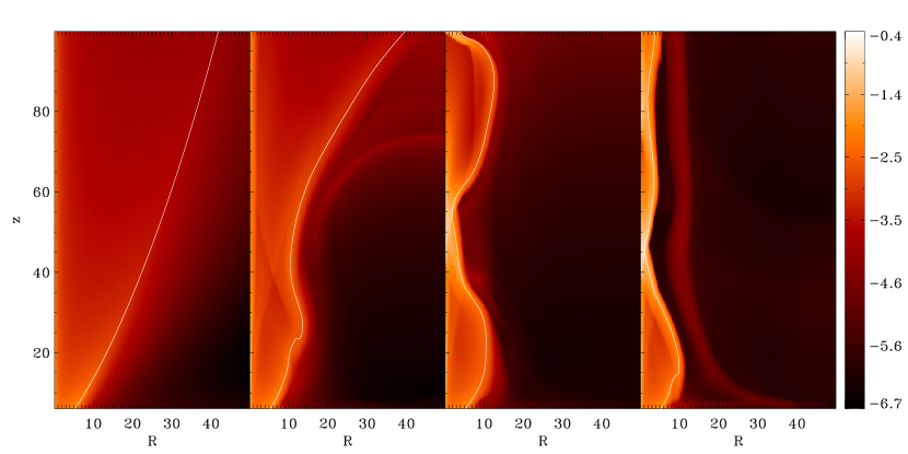
Figure 1: Structure of the flow (logarithmic density plots) for model CD1 at timesteps $t=0,2,3,6\,t_{0}$, respectively. This is an example for the collapse occurring in all test runs except for model ER2. The truncation field line (the magnetic field line with $\alpha=\alpha_{\rm trunc}=0.4$ which is anchored in the lower boundary at $R=5.375$) is also plotted (white line).

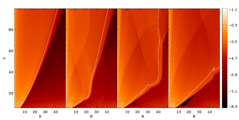
Figure 2: Structure of the flow (logarithmic density plots) for model ER2 at timesteps $t=0,1,2,3\,t_{0}$, respectively. This is the only model without a collapse. The white line is the truncation field line (the magnetic field line with $\alpha=\alpha_{\rm trunc}=0.4$ which is anchored in the lower boundary at $R=5.375$). The positions of the slow- and fast-magnetosonic waves emitted by the truncation field line and of the fast magnetosonic separatrix surface (FMSS) are marked by black lines.

The fact that a new smooth jet surface forms right behind the dent is a promising result, which may be a hint for a new equilibrium and thus a steady solution. However, this couldn’t be tested in these runs, since the solution collapsed.

In Fig. 3 we plot the radii of the jets in models CD1, ER2 and ADO at several values of $z$. These radii correspond to the truncation field line (anchored in the lower boundary where $\alpha=\alpha_{\rm trunc}$ at $R=5.375$), although this is not the outermost field line inside the jet for all timesteps in all models.

In model CD1, the jet radius stays constant until the collapse. The collapse starts at high latitudes (about $z=50$) and then affects the jet further down-stream. After the collapse, the radius varies along the jet length and also with time. A similar structure is also seen in models CD2–CD4 and FL1–FL3 with similar values of the jet radii.

Figure 3: Evolution of the jet radius (radius of the truncation field line) for models CD1, ER2 and also the unchanged analytical solution ADO, at two representative $z$ values above the equatorial plane ($z=10$ and $z=25$ in the models ER2 and ADO; $z=10$ and $z=50$ in the model CD1). The models ADO and ER2 are stationary while the model CD1 collapses.

The time $t_{\rm coll}$ at which the jet collapses is different in each model (Table 1). In models CD1–CD4 testing the influence of numerical resolution and domain size we can clearly see that the size of the computational domain seems to be important for triggering the collapse. The larger the computational domain, the later the collapse occurs. The similarity between models CD2 and CD3 shows that the resulting timescale does not depend on the numerical resolution, or that the coarsest numerical resolution we chose seems to be enough to properly describe the problem.

It is very likely that the collapse is a numerical artefact triggered by the boundary conditions at the outer radial boundary. Since we used “outflow” conditions, all gradients are set to zero at the boundary. This choice affects the radial component of the Lorentz force

$$F_{R}=-\frac{1}{2}\,\frac{\partial\,B_{\phi}^{2}}{\partial\,R}-\frac{B_{\phi}^{2}}{R}-\frac{1}{2}\,\frac{\partial\,B_{Z}^{2}}{\partial\,R}+B_{Z}\,\frac{\partial\,B_{R}}{\partial\,Z}\,,$$ (21)

i.e. it cancels the radial gradient of the magnetic pressure, but it leaves the pinching force (second term on the right-hand side) unaffected. This may result in artificial collimation of the flow (e.g. Ustyugova et al. 1999; Zanni et al. 2007). Only in model ER2, where the toroidal magnetic field component $B_{\phi}$ (not only the density and the $Z$ velocity component) is damped to zero at the outer radial boundary, the collapse can be avoided. Although the simulation time is very short ($3.6\,t_{0}$), we can see that the model is stationary up to this point, after a short period of expansion due to higher thermal and magnetic pressure in the inner region which is also present in the science simulations (see below).

Other effects caused by the very small values of $\rho$ and $v_{Z}$ in the external region as in model CD5 may be present. The fact, whether the outer radial boundary is causally connected with the jet from the very beginning or not, seems to be irrelevant for the presence or absence of the collapse.

In conclusion, it seems to be imperative that either the toroidal magnetic field component $B_{\phi}$ should be very small at the outer radial boundary or that all quantities should be modified self-consistently in order to maintain an equilibrium in the external region.

In all test models, a practical problem occurs: the time step decreases by three up to nine orders of magnitudes, making it impossible to further advance the simulations. This happens in the collapsing models as well as in model ER2. In the latter, all quantities are exponentially damped to very small values close to the outer radial boundary, the large gradient in the last grid cell meets the zero gradient boundary condition in the ghost cells, which triggers leaking of matter into the domain and creating large velocities of all waves close to the boundary. This results in very small timesteps. In order to continue our studies and start a parameter study we are thus forced to “truncate the truncation” as described in the next section.

5 Parameter study of steady solutions

5.1 Initial conditions

In the science models SC1a – SC5, we use the following approach: we modify again all quantities in one of the two components of the outflow, and second, we initialize the external region with another analytical solution with slightly changed parameters. One can show that if $\left[\rho\,(R,Z)\,,p\,(R,Z)\,,\@vec{v}\,(R,Z)\,,\@vec{B}\,(R,Z)\right]$ is a solution of the MHD equations then $\left[\rho\,^{\prime}\,(R\,^{\prime},Z\,^{\prime})\,,p\,^{\prime}\,(R\,^{\prime},Z\,^{\prime})\,,\@vec{v}\,^{\prime}\,(R\,^{\prime},Z\,^{\prime})\,,\@vec{B}\,^{\prime}\,(R\,^{\prime},Z\,^{\prime})\right]$ with

$$R\,^{\prime}=\lambda_{1}\,R\,, Z\,^{\prime}=\lambda_{1}\,Z\,,$$

$$\@vec{B}\,^{\prime}=\lambda_{2}\,\@vec{B}\,, \@vec{v}\,^{\prime}=\sqrt{\frac{\lambda_{3}}{\lambda_{1}}}\,\@vec{v}\,,$$

$$\rho\,^{\prime}=\frac{\lambda_{1}\,\lambda_{2}^{2}}{\lambda_{3}}\,\rho\,, p\,^{\prime}=\lambda_{2}^{2}\,p\,,$$

$$\mathcal{M}\,^{\prime} = \lambda_{3}\,\mathcal{M}$$ (22)

is also a solution of the same set of equations. These transformations have also implications for the integrals of motion

$$\Psi_{A}\,^{\prime}(A)=\lambda_{2}\,\sqrt{\frac{\lambda_{1}}{\lambda_{3}}}\,\Psi_{A}\,(A)\,, \Omega\,^{\prime}(A)=\sqrt{\frac{\lambda_{3}}{\lambda_{1}^{3}}}\,\Omega(A)\,,$$

$$L\,^{\prime}(A)=\sqrt{\lambda_{1}\,\lambda_{3}}\,L(A)\,, E\,^{\prime}(A)=\frac{\lambda_{3}}{\lambda_{1}}\,E(A)\,,$$

$$Q\,^{\prime}(A) = \lambda_{2}^{2-2\,\Gamma}\,\left(\frac{\lambda_{3}}{\lambda_{1}}\right)^{\Gamma}\,Q(A)\,.$$ (23)

Since in our case, both solutions should have the same central object, we set $\lambda_{3}=1$. We also ignore the scaling of $R$ and $Z$, i.e. we do not initialize e.g. $\rho\,^{\prime}\,(R\,^{\prime},Z\,^{\prime})$, but $\rho\,^{\prime}\,(R,Z)$ in the outer region. Formally, this is not a solution of the MHD equations, since the gravity term explicitly depends on the length scale. In our case, however, the gravitational force is small compared to the other forces, thus this slight inconsistency is unimportant.

We match both solutions by using the function

$$\mathcal{Q}=\mathcal{Q}_{\rm jet}\,\exp[-(\alpha/\alpha_{\rm trunc})^{2}]+\mathcal{Q}_{\rm ext}\,\left(1-\exp[-(\alpha/\alpha_{\rm trunc})^{2}]\right)$$ (24)

for all quantities.

Note that model ER2 can be also described by this ansatz, when we set $\mathcal{Q}_{\rm ext}=0$ , i.e. simply damp all quantities with the exponential factor, or equivalently if we set $\lambda_{1}\to\infty$ and $\lambda_{2}\to 0$. However, this truncation led to problems with the time step (see Sec. 4). In model SC1a, we try to mimic this behavior less drastically by setting $\lambda_{1}=10^{3}$ and $\lambda_{2}=10^{-3}$ ($v\,^{\prime}=10^{-3/2}\,v$, $B\,^{\prime}=10^{-3}\,B$, $p\,^{\prime}=10^{-6}\,p$, $\rho\,^{\prime}=10^{-3}\,\rho$).

In Eqs. (5.1)–(5.1), several special cases can be distinguished, coinciding with combinations of $\lambda_{1}$ and $\lambda_{2}$ where quantities or integrals remain unchanged in both solutions:

1. If $\lambda_{1}=1$, $R$, $Z$, $\@vec{v}$, $\Omega(A)$, $L(A)$ and $E(A)$ remain the same.

2. If $\lambda_{2}=1$, $\@vec{B}$ and $p$ are the same.

3. If $\sqrt{\lambda_{1}}\,\lambda_{2}=1$, $\rho$ and $\Psi_{A}\,(A)$ remain the same.

The additional case, where $\lambda_{1}=\lambda_{2}=1$, is of course identical with the unchanged analytical solution of V00 and therefore uninteresting in this study. For each choice of $\lambda_{1}$ and $\lambda_{2}$ we can create two different models, depending on whether the unchanged solution is inside or outside the solution with primed quantities.

In model SC2, we use the scaling parameters $\lambda_{1}=100$ and $\lambda_{2}=0.1$ (case 3.), i.e $v\,^{\prime}=0.1\,v$, $B\,^{\prime}=0.1\,B$, $p\,^{\prime}=0.01\,p$, $\rho\,^{\prime}=\rho$, in the exterior region. In model SC3 we use the same scaling parameters, but apply the primed solution in the interior. In model SC4, our combination is $\lambda_{1}=1$ and $\lambda_{2}=0.1$ (case 1.) in the exterior and in model SC5 in the interior, leading to $v\,^{\prime}=v$, $B\,^{\prime}=0.1\,B$, $p\,^{\prime}=0.01\,p$, $\rho\,^{\prime}=0.01\,\rho$.

Table 2: List of numerical science models

Name	Grid size	Resolution	$t_{\rm end}$	Description
SC1a	[0,50] $\times$ [6,100]	200 $\times$ 400	250.0	$\alpha_{\rm trunc}=0.4$, external analytical solution $\lambda_{1}=10^{3}$, $\lambda_{2}=10^{-3}$
SC1b	[0,50] $\times$ [6,100]	200 $\times$ 400	250.0	$\alpha_{\rm trunc}=0.2$, external analytical solution $\lambda_{1}=10^{3}$, $\lambda_{2}=10^{-3}$
SC1c	[0,50] $\times$ [6,100]	200 $\times$ 400	250.0	$\alpha_{\rm trunc}=0.1$, external analytical solution $\lambda_{1}=10^{3}$, $\lambda_{2}=10^{-3}$
SC1d	[0,50] $\times$ [6,100]	200 $\times$ 400	250.0	$\alpha_{\rm trunc}=0.01$, external analytical solution $\lambda_{1}=10^{3}$, $\lambda_{2}=10^{-3}$
SC1e	[0,50] $\times$ [6,100]	200 $\times$ 400	250.0	$\alpha_{\rm trunc}=0.001$, external analytical solution $\lambda_{1}=10^{3}$, $\lambda_{2}=10^{-3}$
SC2	[0,50] $\times$ [6,100]	200 $\times$ 400	250.0	$\alpha_{\rm trunc}=0.4$, external analytical solution $\lambda_{1}=100$, $\lambda_{2}=0.1$
SC3	[0,50] $\times$ [6,100]	200 $\times$ 400	250.0	same as model SC2, but solutions are swapped
SC4	[0,50] $\times$ [6,100]	200 $\times$ 400	250.0	$\alpha_{\rm trunc}=0.4$, external analytical solution $\lambda_{1}=1$, $\lambda_{2}=0.1$
SC5	[0,50] $\times$ [6,100]	200 $\times$ 400	250.0	same as model SC4, but solutions are swapped

5.2 Results of the science simulations

5.2.1 Structure of the flow

As expected a priori, the flows behave qualitatively very differently, depending on whether the scaled-down solution is inside or outside the original one.

In the cases where the quantities are scaled down in the exterior region, the opening angle of the flow increases, see Figs. 4 and 5). The jet surface is pushed outwards by the higher thermal and magnetic pressure in the inner region, which also dilutes while expanding. A new equilibrium is established within several $t_{0}$ and is stable for at least 250 $t_{0}$. The final opening angles seen in the density plots seem to be too large for calling the flow a collimated jet. Using the truncation field line plotted in the figures, we find angles of about 40^∘–50^∘ in models SC1a – SC2 and model SC4. In paper II of this series, we assess the “apparent” opening angle by calculating emission maps and find that the emitting region is very collimated in all models (the opening angles are of the order of 10^∘–20^∘).

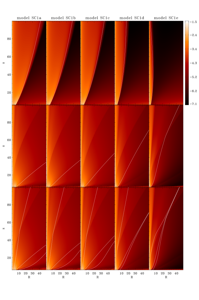
Figure 4: Structure of the flow (logarithmic density plots) for models SC1a – SC1e (from left to right) at timesteps $t=0$ (top), $t=25$ (middle) and $t=50\,t_{0}$ (bottom), respectively. Also plotted is the magnetic field line anchored in the lower boundary where $\alpha=\alpha_{\rm trunc}$ (white line)). At $t=50\,t_{0}$, we also plot the two field lines with half and twice the radius of that of the truncation field line which are used in Sec. 5.2.5, Fig. 14

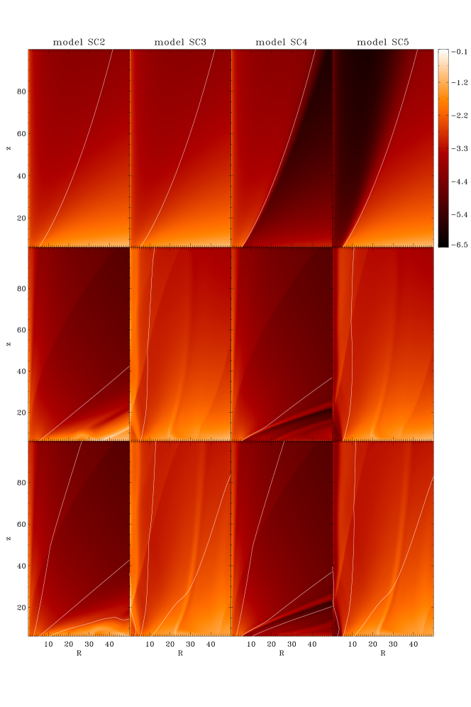
Figure 5: Structure of the flow (logarithmic density plots) for models SC2 – SC5 (from left to right) at timesteps $t=0$ (top), $t=25$ (middle) and $t=50\,t_{0}$ (bottom), respectively. Also plotted is the magnetic field line anchored in the lower boundary where $\alpha=\alpha_{\rm trunc}$ (white line). At $t=50\,t_{0}$, we also plot the two field lines with half and twice the radius of that of the truncation field line which are used in Sec. 5.2.5, Fig. 14

If all quantities are reduced in the internal region (models SC3 and SC5), then the opening angle decreases. Again a new equilibrium is established which is stable for at least 250 $t_{0}$, see Fig. 5. The final opening angles in these runs are very small, around 5^∘. New features are several shocks, the innermost of which is also collimated following magnetic field lines.

The expansion of the flow in models SC1a–SC1e, SC2 and SC4 (Fig. 4), and the collimation in models SC3 and SC5 (Fig. 5) is clearly visible in the evolution of the jet radius. While the jet radius is very similar in both models showing the collimation, a clear trend can be identified in the first case: the largest expansion occurs in model SC4, followed by the models SC1a, SC1b, SC2, SC1c, SC1d and SC1e. Surprisingly model SC1a, which is the model with the smallest values of thermal pressure and magnetic field in the outer region, is not the one with the highest expansion. Although models SC2 and SC4 have the same scalings for thermal pressure and magnetic field, they show different degrees of expansion.

In models SC3 and SC5, again two shocks are present which move outwards. When the inner region shrinks due to its lower thermal and magnetic pressure compared to the exterior, two waves propagate towards larger radii emitted from the truncation field line. One wave travels faster than the other, and since both waves compress the medium, they seem to be again a slow- and a fast-magnetosonic wave. The fast wave has reached the outer radial boundary at 50 $t_{0}$, only its part at lower latitudes ($z<20$) is still visible inside the domain. The slow wave stops when its lower part (at $z=6$) reaches $R=22$, which is exactly the location where the slow-magnetosonic critical surface crosses the lower boundary. Since the slow-magnetosonic wave cannot cross the corresponding critical surface, it is then attached to this point and develops a standing and steepening shock inside the domain. A third shock, which is also present in the model ADO, develops at the fast magnetosonic separatrix surface (FMSS). This weak shock acts as a ”wall” protecting the sub-fast flow from the imposed modifications close to the axis (GVT06, M08). Note that the poloidal field lines develop a bend at the position of all shocks.

In models SC1a and SC1b, a small dip is present after about 70 $t_{0}$ and 150 $t_{0}$, respectively. Before this dip, the radii are almost constant, as well as in the other models (Fig. 6, top, dashed line).

5.2.2 Are there boundary effects in the science runs?

We have also run models SC1a’, SC3’ and SC4’ with a larger domain ([0,100]$\times$[6,200]) to check whether the science runs presented above are affected by the boundaries.

The results concerning the jet radii measured with the truncation field line are only changed by a few percent in models SC1a’ (with respect to the constant part in model SC1a) and SC4’, with less effects in model SC4’ than in model SC1a’, see Fig. 6. The small dip seen in model SC1a is smoothed out, thus it was indeed created by boundary effects as suspected. In model SC3’, larger changes exist at higher $z$ values ($z>75$) after about 50 $t_{0}$. While in model SC3, the radii decrease, they stay constant in model SC3’.

Figure 6: Comparison of the jet radius evolution in models SC1a and SC1a’, models SC3 and SC3’ and models SC4 and SC4’ (black dashed: unprimed models, red solid: primed models)

Therefore, throughout the remainder of the paper, the results of all runs at 50 $t_{0}$ will be considered as “real” final stationary states of the solutions.

5.2.3 Force balance along the jet boundary

The interplay between the $R$ components of the pressure gradient and the Lorentz force (which, as expected, always dominates in those radially self-similar disk-wind models) is responsible for collimating the flow or triggering its expansion in all models (see Figs. 7 – 8). In the expanding models SC1a–SC1e and SC2, the Lorentz force and the pressure gradient are directed outwards, while they are directed inwards in the models SC3 and SC5. The first is also true for model SC4, the pressure gradient turns inwards between $z=7$ and $z=14$. Furthermore, in all models except for SC4, the pressure gradient is only important at lower $z$ values between 6 – 8.

Figure 7: $R$ (top) and $z$ (bottom) components of forces along the jet boundary at the final simulated timestep (at 50 $t_{0}$) in models SC1a. The components are measured at the truncation field line plotted in previous figures and multiplied by $R_{\rm fl}^{3}$ with $R_{\rm fl}$ the local cylindrical radius of the field line

Figure 8: Same as in Fig. 7, but for model SC3.

5.2.4 Quantities at the outer axial boundary and the properties of the jet

In Figs. 9–13, all eight magnetohydrodynamic quantities are plotted along the outer axial boundary at $z=100$ for our models SC1a – SC5. In each panel, we show the initial profile of our model (solid line), the profile of the unchanged analytical solution (dash-dotted line) and the final profile at $t=50\,t_{0}$ (dashed line). One can clearly see how the initial profile follows the analytical solution in the interior region and is damped in the exterior in models SC1a–SC2 and SC4 and vice versa in models SC3 and SC5.

In models SC1a–SC1e, SC2 and SC4, at large radii, most profiles have a similar shape as the unchanged analytical solution, we started with. The original break is mostly leveled out in all of the profiles. However, at small radii ($R<7$) the final solution deviates drastically. This is expected, since the analytical solution is modified close to the axis to avoid the intrinsic singularities. In density, pressure, axial ($z$) and toroidal ($\phi$) velocity components, as well as in axial magnetic field, a peak is present where all quantities are higher than at larger radii ($R>7$). The radial ($R$) velocity and magnetic field components and the toroidal magnetic field on the other hand show strong deviations from the initial profiles with strong declines close to the axis in the former two quantities and a steep rise and a minimum at about $R=4$ in the latter. The relative height of the central peak, the height of the remaining break and the depth of the minimum in $B_{\phi}$ are different across the five models. Although the models SC2 and SC4 are special cases, where the density and the velocity, respectively, is unchanged in the inner and outer region, the final profiles in all models including these two are similar.

In models SC3 and SC5, the initial profiles have to be changed dramatically to stop the decrease of the opening angle and the collapse of the jet. The profiles are much more complicated and less smooth than in the other five cases described above. Again some final profiles show a similar shape as the unchanged analytical solution at large radii. However, superimposed on all of them is a shock structure with jumps in density, pressure, radial magnetic field and toroidal velocity (at about $R=4$, $R=13$, $R=25$, and $R=37$ in model SC3). The radial magnetic field changes sign at the innermost shock where the density and pressure rise steeply and a minimum in axial velocity is present in model SC3. In model SC5, the radial magnetic field also changes sign at the innermost shock which is, however, now characterized by a steep decline in density and a steep rise in axial velocity.

Figure 9: Quantities at the outer axial boundary in model SC1a: density (top left), pressure (top right), velocity components in $R$ (second row, left), $z$ (second row, right) and $\phi$ (third row, left), magnetic field components in $R$ (third row, right), $z$ (bottom left) and $\phi$ (bottom right); given are the initial profiles (solid), the final profiles at $50\,t_{0}$ (dashed) and the profiles in the unchanged analytical solution of V00.

Figure 10: Same as in Fig. 9, but for the model SC2.

Figure 11: Same as in Fig. 9, but for the model SC3.

Figure 12: Same as in Fig. 9, but for the model SC4.

Figure 13: Same as in Fig. 9, but for the model SC5.

5.2.5 The integrals of motion

In Fig. 14, we plot the integrals of motion given by Eqs. (6) – (9), along the truncation field line at the interface of both regions, along an inner field line which is anchored at half of the radius of the truncation field line, and along an outer field line anchored at twice the radius.

When we compare the integrals along the inner field line in the models SC1a – SC1e, SC2 and SC4 with those in the analytical model ADO, we can see that the flow in the inner region is very similar to the analytical solution we started with. An exception is model SC1e, where the inner field line is already very close to the symmetry axis, i.e. our modifications there affect the integrals of motion. All integrals of motion converge smoothly to an asymptotic value. The deviation from this value are within 6 % for $z$ values above 20.

In the remaining models SC3 and SC5, the behavior of the integrals of motion along the inner field line is very different to the other models, but similar to each other. At about $z=50$, peaks and dips are visible in all integrals, however, with the most pronounced in $Q$.

In the outer region, all integrals seem to converge in models SC1a–SC1e, SC2, SC3 and SC5. The turnovers in model SC2 are a result of a turnover in the field line itself. In model SC4, $L$ and $\Psi_{A}$ have already converged, the other integrals still vary. In conclusion, in most of our models also the external region reaches a steady state.

Figure 14: Integrals of motion $\Psi_{A}\,(A)$, $\Omega(A)$, $L(A)$, $E(A)$ and $Q(A)$, normalized to their values at their end point, where they leave the domain, along the truncation field line (left), along a second field line anchored at half of the radius (middle) and along a third field line anchored at twice of the radius (right) for models SC1a, SC2 – SC5 and ADO (from top to bottom).

5.2.6 Topology of the current lines

In Fig. 15, we plot the poloidal currents for our nine science models SC1a – SC5. In model ADO, as well as in the inner region of models SC1a–SC2 and SC4, which remains unchanged with respect to the analytical solution, a re-adjusted FMSS is visible as shock in the density plots (Figs. 4 – 5, cf. GVT06 and M08). The currents in these models are counterclockwise upstream and downstream of the FMSS. Only along the FMSS the current close, i.e. the lines are clockwise. This distribution of currents, and in particular the direction of the resulting $\@vec{J}_{\rm p}\times\@vec{B}_{\phi}$ force, is consistent with the decollimation and deceleration that the flow experiences as it passes through the shock. Thus, one of the effects of the new FMSS is to bend the streamlines away from the z-axis avoiding the overcollimation property of the original analytical solution. The collimation and decollimation processes that can be derived from such a plot are also discussed in GVT06. Towards the outer region, the morphology of the current lines is distorted and of completely different topology. In models SC4 and SC1a–SC1e, the outer region is separated by a second shock with a current sheet from the inner region.

In models SC3 and SC5, the FMSS is also present. Again at the shock, a current sheet separates two region with counterclockwise currents. Furthermore, closer to the rotation axis, another current sheet forms an X shape with the FMSS at $(R,z)=(5,30)$ and a third current sheet in the lower right corner of the domain develops.

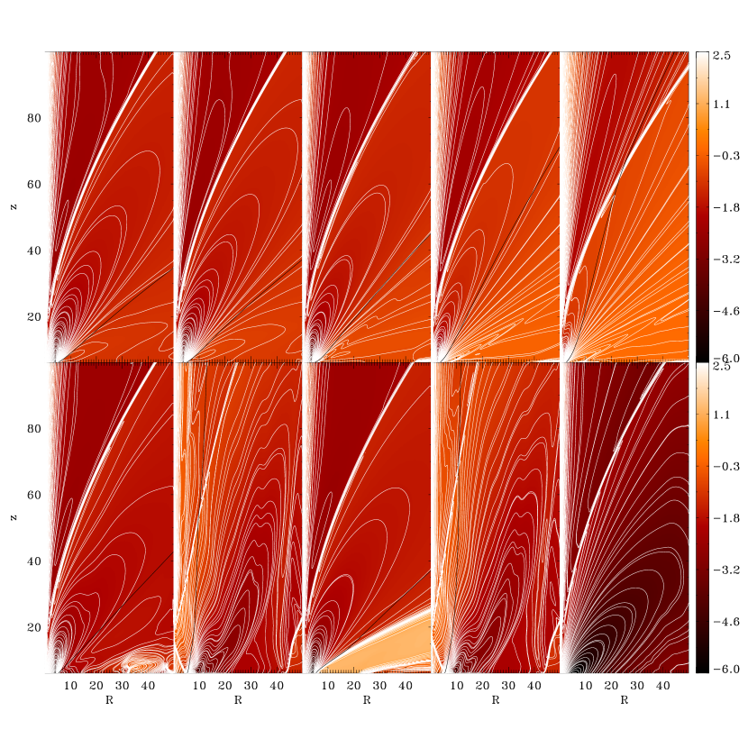
Figure 15: Poloidal currents $R\,B_{\phi}=const$ of models SC1a–SC1e (top) and models SC2–SC5 and ADO (bottom) at the final timestep (at 50 $t_{0}$) are plotted.

6 Summary

In this paper, we have studied the effects of imposing an outer radius of the underlying accreting disk, and thus also of the outflow, on the topology, structure and time-dependence of a well studied radially self-similar analytical solution (V00). We matched an unchanged and a scaled-down analytical solution of V00 and found in all these cases steady two-component solutions.

We showed that the boundary between both solutions is always shifted towards the solution with reduced quantities. Especially, the reduced thermal and magnetic pressure change the perpendicular force balance at the “surface” of the flow. In the models where the scaled-down analytical solution is outside the unchanged one, the inside solution converges to another analytical solution with different parameters. In the models where the scaled-down analytical solution is inside the unchanged one, the whole two-component solution changes dramatically to support the flow from collapsing totally to the symmetry axis.

A result of the modification of the analytical solution at the symmetry axis is the formation of a weak shock at the fast magnetosonic separatrix surface (FMSS) which shields the flow upstream of the FMSS from the imposed modifications close to the axis. A result of the truncation of the analytical solution along some poloidal field line is the formation of two compressive MHD shocks: a fast shock that travels quickly downstream outside of the computational domain and a slow shock which as it travels downstream with lower speed, it is locked precisely at the position of the lower computational z-boundary where the analytical slow surface meets this boundary.

Our truncated disk-wind solutions are stable for more than 50 $t_{0}$, i.e. several orbital periods at the truncation radius. These solutions may be relevant to describe observed jets, since the jet radii are too large in the untruncated analytic disk outflow solution, with respect to observed jet widths. We also provide all quantities at the outer $z$ boundary which can now be used as boundary conditions for jet propagation studies.

In the following paper II, we calculate emission maps corresponding to such truncated disk-models and compare them with observations.