Quasinormal modes of RN black hole space time with cosmic string in a Dirac field

Abstract

We evaluate quasinormal mode frequencies for RN black hole space times with cosmic string perturbed by a massless Dirac field, using Pöschl-Teller potential method. We find that only in the case of RN black hole having small charge, the effect due to cosmic string will dominate when perturbed by a negatively charged Dirac field, but if we are perturbing with positively charged dirac field decay will be less in the case of black hole having cosmic string compared to the RN black hole without string..

Received (Day Month Year)Revised (Day Month Year)

PACS numbers:04.70.-s, 04.62.+v , 11.27.+d

1 Introduction

There has been a great interest in the long standing issue in classical relativistic theory of gravitation: small perturbations or quasinormal modes associated with black holes. The question of stability of black hole was first treated by Regge and Wheeler [1] who investigated linear perturbations of the exterior Schwarzschild space time. Further work [2] on this problem led to the study of quasinormal modes which is believed as a characteristic sound of black holes. Quasinormal modes (QNMs) describe the damped oscillations under perturbations in the surrounding geometry of a black hole with frequencies and damping times of oscillations entirely fixed by the black hole parameters. The study of QNMs became an intriguing subject of discussion for last few decades [3, 4, 5, 6] and references therein. QNMs carry unique finger prints of black holes and it is well known that they are crucial in studying the gravitational and electromagnetic perturbations around black hole space times. They are also seem to have an observational significance as the gravitational waves produced by the perturbations, in principle, can be used for unambiguous detection of black holes. This motivates us to study the quasinormal mode spectra of black holes.

The motivation of the present work is to study the signature of cosmic strings on QNMs. It has been recognized that certain gauge theories allow the possibility of topological defects, such as strings, magnetic poles etc and that these defects represent objects which might have been created in the very early universe [7]. Cosmic strings are strand of matter which could be created in a cosmological phase transition. In 1976 Kibble suggested the possibility of strings in the early universe[8]. These cosmic strings might be responsible for large-scale structure in the universe. Although little is known about these strings, it is clear that they raise a number of issues in fundamental physics and thus it seems to be of particular interest, both as a possible ”seed” for galaxy formation [9, 10] and as a possible gravitational lens[11].

The QNMs of scalar perturbations around a Schwarzschild black hole pierced by a cosmic string was done earlier [12]. We have evaluated earlier[13] quasinormal mode frequencies for Schwarzschild, RN extremal, SdS and near extremal SdS black hole space times with cosmic string perturbed by a massless Dirac field. In this paper we study the influence of cosmic string on the QNMs of RN black hole background space time which are perturbed by a massless Dirac field. In section II, we consider the Dirac equation in a RN black hole space time with a cosmic sting and its deduction into a set of second order differential equations. In Section III we evaluate the Dirac quasinormal frequencies for the massless case using Pöschl-Teller potential method for RN black holes.

2 RN black hole with cosmic string space time for a Dirac field

The metric describing a charged spherically symmetric black hole(RN) with a cosmic string can be written as[14],

$$ds^{2}=f(r)dt^{2}-\frac{dr^{2}}{f\left(r\right)}-r^{2}d\theta^{2}-b^{2}r^{2}\sin^{2}\theta d\phi^{2}.$$ (1)

Here $f(r)=1-\frac{2M}{r}+\frac{Q^{2}}{r^{2}}$, $Q$ and $M$ are representing the electric charge and the mass of the black hole. This can be constructed by removing a wedge, which is done by requiring that the azimuthal angle around the axis runs over the range $0<\phi^{\prime}<2\pi b$, with $\phi^{\prime}=b\phi$ where $\phi$ runs over zero to $2\pi$. Here $b=1-4\check{\mu}$ with $\check{\mu}$ being the linear mass density of the string. Using the procedure adopted in reference [15] the Dirac equation in the presence of an electromagnetic interaction in a general background space time can be written as,

$$\left(\gamma^{\mu}(\partial_{\mu}-\Gamma_{\mu}-\imath eA_{\mu})+m\right)\Psi=0,$$ (2)

where $m$ and $e$ are the the mass and charge of the Dirac field, $A_{\mu}$ is the electro magnetic potential which can be written as,

$$A_{\mu}=\left(\frac{Q}{r},0,0,0\right),$$ (3)

Here

$$\gamma^{\mu}=g^{\mu\nu}\gamma_{\nu},$$ (4)

and

$$\gamma_{\nu}=e_{\nu}^{a}\gamma_{a},$$ (5)

where $\gamma^{a}$ are the Dirac matrices,

$$\gamma_{0}=\left[\begin{array}[]{cc}\imath&0\\ 0&-\imath\end{array}\right],\gamma_{i}=\left[\begin{array}[]{cc}0&\sigma_{i}\\ \sigma_{i}&0\end{array}\right],$$ (6)

and $\sigma_{i}$ are the Pauli matrices. $e_{\nu}^{a}$ is the tetrad given by,

$$e_{t}^{t}=f^{\frac{1}{2}};e_{r}^{r}=\frac{1}{f^{\frac{1}{2}}};e_{\theta}^{\theta}=r,e_{\phi}^{\phi}=br\sin\theta.$$ (7)

The inverse of the tetrad $e_{\nu}^{a}$ is defined by,

$$g^{\mu\nu}=\eta^{ab}e_{a}^{\mu}e_{b}^{\nu},$$ (8)

with $\eta^{ab}=diag(-1,1,1,1)$, the Minkowski metric. The spin connection $\Gamma_{\mu}$ is given by

$$\Gamma_{\mu}=-\frac{1}{2}[\gamma_{a},\gamma_{b}]e_{\nu}^{a}e^{b\nu}_{;\mu},$$ (9)

where $e^{b\nu}_{;\mu}=\partial_{\mu}e^{b\nu}+\Gamma_{\kappa\mu}^{\nu}e^{b\kappa}$ is the covariant derivative of $e^{b\nu}$. The spin connections for the above metric are obtained as,

$$\Gamma_{t} = \frac{1}{4}\gamma_{1}\gamma_{0}\frac{\partial f\left(r\right)}{\partial r},$$ (10)

$$\Gamma_{r} = 0,$$ (11)

$$\Gamma_{\theta} = \frac{1}{2}\gamma_{1}\gamma_{2}f^{\frac{1}{2}}\left(r\right),$$ (12)

$$\Gamma_{\phi} = \frac{1}{2}\gamma_{2}\gamma_{3}b\cos\theta+\frac{1}{2}\gamma_{1}\gamma_{3}b\sin\theta f^{\frac{1}{2}}\left(r\right).$$ (13)

Substituting the spin connections in Eq. (2) we will get ,

$$[\frac{-\gamma_{0}}{f^{\frac{1}{2}}}(\frac{\partial}{\partial t}-\imath\frac{eQ}{r})+\gamma_{1}f^{\frac{1}{2}}(\frac{\partial}{\partial r}+\frac{1}{r}+\frac{1}{4{f(r)}}{\frac{\partial f}{\partial r}})+\frac{\gamma_{2}}{r}(\frac{\partial}{\partial\theta}+\frac{1}{2}\cot\theta)+\frac{\gamma_{3}}{br\sin\theta}\frac{\partial}{\partial\phi}+m]\Psi(t,r,\theta,\phi)=0,$$ (14)

Using the transformation $\Psi(t,r,\theta,\phi)=\frac{\exp(-\imath Et)}{rf^{\frac{1}{4}}{\sin\theta}^{\frac{1}{2}}}\chi(r,\theta,\phi)$, Eq.(14) becomes,

$$[\frac{-E-\frac{eQ}{r}}{f^{\frac{1}{2}}}\frac{\partial}{\partial t}+\frac{1}{\imath}\gamma_{0}\gamma_{1}f^{\frac{1}{2}}(\frac{\partial}{\partial r})+\frac{\gamma_{1}}{\imath r}\gamma_{1}\gamma_{0}(\gamma_{2}\frac{\partial}{\partial\theta} +$$

$$\frac{\gamma_{3}}{b\sin\theta}\frac{\partial}{\partial\phi})-\imath\gamma_{0}m]\chi(r,\theta,\phi)=0.$$ (15)

Dirac equation can be separated out into radial and angular parts by the following substitution,

$$\chi(r,\theta,\phi)=R(r)\Omega(\theta,\phi).$$ (16)

The angular momentum operator is introduced as, [15]

$$\mathbf{K}_{\left(b\right)}=-\imath\gamma_{1}\gamma_{0}\left(\gamma_{2}\partial_{\theta}+\gamma_{3}\left(b\sin\theta\right)^{-1}\partial_{\phi}\right),$$ (17)

such that,

$$\mathbf{K}_{(b)}\Omega(\theta,\phi)=k_{b}\Omega(\theta,\phi),$$ (18)

where the eigenvalues of $\mathbf{K}_{(b)}$ are $k_{b}=\frac{k}{b}$. Here k is a positive or a negative nonzero integer with $l=|k+\frac{1}{2}|-\frac{1}{2}$, where $l$ is the total orbital angular momentum. The cosmic string presence is codified in the eigenvalues of the angular momentum operator[16]. Substituting Eqs.(16) and (18) in Eq.(15), we will get radial equation which contains $\gamma_{0}$ and $\gamma_{1}$. As $\gamma_{0}$ and $\gamma_{1}$ can be represented by $2\times 2$ matrices, we write the radial factor $R(r)$ by a two component spinor notation,

$$R(r)=\left[\begin{array}[]{c}F\\ G\end{array}\right].$$ (19)

Then the radial equation in F an G are given by,

$$f\frac{dG}{dr}+f^{\frac{1}{2}}\frac{k_{b}}{r}G+f^{\frac{1}{2}}mF=(E+\frac{eQ}{r})F,$$ (20)

$$f\frac{dF}{dr}-f^{\frac{1}{2}}\frac{k_{b}}{r}F+f^{\frac{1}{2}}mG=-(E+\frac{eQ}{r})G.$$ (21)

Let us have a co-ordinate change given by,

$$dr_{\ast}=\frac{dr}{f}.$$ (22)

Eq.(20) and Eq.(21) then become,

$$\frac{\partial}{\partial r_{\ast}}\left[\begin{array}[]{c}G\\ F\end{array}\right]+f^{\frac{1}{2}}\left[\begin{array}[]{cc}\frac{k_{b}}{r}&m\\ m&-\frac{k_{b}}{r}\end{array}\right]\left[\begin{array}[]{c}G\\ F\end{array}\right]=\left[\begin{array}[]{cc}0&E+\frac{eQ}{r}\\ -E-\frac{eQ}{r}&0\end{array}\right]\left[\begin{array}[]{c}G\\ F\end{array}\right].$$ (33)

Defining,

$$\left[\begin{array}[]{c}\hat{G}\\ \hat{F}\end{array}\right]=\left[\begin{array}[]{cc}\cos\frac{\theta}{2}&-\sin\frac{\theta}{2}\\ \sin\frac{\theta}{2}&\cos\frac{\theta}{2}\end{array}\right]\left[\begin{array}[]{c}G\\ F\end{array}\right],$$ (34)

where

$$\theta=\tan^{-1}(\frac{mr}{|k_{b}|}).$$ (35)

Eq.(33) becomes,

$$\frac{\partial}{\partial r_{\ast}}\left[\begin{array}[]{c}\hat{G}\\ \hat{F}\end{array}\right]+f^{\frac{1}{2}}\sqrt{\left(\frac{k_{b}}{r}\right)^{2}+m^{2}}\left[\begin{array}[]{cc}1&0\\ 0&-1\end{array}\right]\left[\begin{array}[]{c}\hat{G}\\ \hat{F}\end{array}\right]$$ (42)

$$=-E\left[1+\frac{1}{2E}\frac{fm|k_{b}|+}{{{k_{b}}^{2}+m^{2}r^{2}}}++\frac{eQ}{r}\right]\left[\begin{array}[]{cc}0&-1\\ 1&0\end{array}\right]\left[\begin{array}[]{c}\hat{G}\\ \hat{F}\end{array}\right].$$ (47)

By making another change of the variable;

$$d\hat{r}_{\ast}=\frac{dr_{\ast}}{\left[1+\frac{1}{2E}\frac{fmk_{b}}{{k_{b}^{2}+m^{2}r^{2}}}+e\frac{Q}{Er}\right]}.$$ (48)

Eq.(47) can be simplified to,

$$\frac{\partial}{\partial\hat{r}_{\ast}}\left[\begin{array}[]{c}\hat{G}\\ \hat{F}\end{array}\right]+\frac{f^{\frac{1}{2}}\sqrt{\left(\frac{k_{b}}{r}\right)^{2}+m^{2}}}{\left[1+\frac{1}{2E}\frac{fm|k_{b}|}{{k_{b}^{2}+m^{2}r^{2}}}+e\frac{Q}{Er}\right]}\left[\begin{array}[]{cc}1&0\\ 0&-1\end{array}\right]\left[\begin{array}[]{c}\hat{G}\\ \hat{F}\end{array}\right]=E\left[\begin{array}[]{cc}0&1\\ -1&0\end{array}\right]\left[\begin{array}[]{c}\hat{G}\\ \hat{F}\end{array}\right],$$ (49)

i.e,

$$\frac{\partial}{\partial\hat{r}_{\ast}}\left[\begin{array}[]{c}\hat{G}\\ \hat{F}\end{array}\right]+W\left[\begin{array}[]{c}\hat{G}\\ -\hat{F}\end{array}\right]=E\left[\begin{array}[]{c}\hat{F}\\ -\hat{G}\end{array}\right],$$ (50)

where

$$W=\frac{f^{\frac{1}{2}}\sqrt{\left(\frac{k_{b}}{r}\right)^{2}+m^{2}}}{\left[1+e\frac{Q}{Er}+\frac{1}{2E}\frac{fmk_{b}}{{k_{b}^{2}+m^{2}r^{2}}}\right]}.$$ (51)

Thus from Eq.(50), we will get coupled equations for $\hat{G}$ and $\hat{F}$ which are given bellow,

$$-\frac{\partial^{2}\hat{F}}{\partial\hat{r}_{\ast}^{2}}+V_{1}\hat{F}=E^{2}\hat{F},$$ (52)

$$-\frac{\partial^{2}\hat{G}}{\partial\hat{r}_{\ast}^{2}}+V_{2}\hat{G}=E^{2}\hat{G},$$ (53)

where

$$V_{1,2}=\pm\frac{\partial W}{\partial\hat{r}_{\ast}}+W^{2}.$$ (54)

From the equations Eqs (52) and (53), we can evaluate the corresponding quasinormal mode frequencies for various black hole space time. Here $V_{1}$ and $V_{2}$ are the super symmetric partners derived from the same super potential $W$ [17]. It has been shown that potentials related in this way possess the same spectra of quasi-normal mode frequencies.

3 Quasinormal mode frequencies

We shall evaluate the quasi-normal frequencies for RN black hole space times perturbed by a massless Dirac field. For massless case, i.e, $m=0$, the equation for the potential in Eq.(54) becomes,

$$V=f\left(1+e\frac{Q}{Er}\right)\frac{\partial}{\partial r}\left(f^{\frac{1}{2}}\frac{k_{b}}{r\left(1+e\frac{Q}{Er}\right)}\right)$$

$$+f\left(\frac{k_{b}}{r}\right)^{2}\frac{1}{\left(1+e\frac{Q}{Er}\right)^{2}},$$ (55)

where we have avoided the subscript of $V_{1}$. Here we take $Q$ as always positive and the sign of $e$ will change to positive or negative so that the positive sign of $e$ actually means that the product $eQ>0$ and vice versa.

Figure 1: Variation of effective potential for Dirac field with m=0 k=3, e=0.1, E=1 and Q=0(doted line), 0.3(solid line), 0.6(dashed line)and 0.9(bold line). for each b value(0.1, 0.5 and 1)

The effective potential as a function of r is plotted in Fig.1. We can see that the dependence of V on $Q$ is strong and the peak of the potential increases faster and faster with Q. When the value of $b$ is changed form $b=1$ to $b=0.5$ and to $b=0.1$ the peak of the potential is increased, i.e, when the cosmic string is present the height of the potential barrier is increased.

Now we shall evaluate the QNMs using Pöschl-Teller potential approximation proposed by Ferrari and Mashhoon, the Pöschl-Teller potential [18] is given by,

$$V_{PT}=\frac{V_{0}}{\cosh^{2}\left(\frac{r^{\star}}{b}\right)}.$$ (56)

The quantity $V_{0}$ and $b$ are given by the height and curvature of the potential at its maximum($r=r_{max}$). Thus

$$V_{0}=V_{r_{max}},\frac{1}{b^{2}}=-\frac{1}{2V_{0}}\left[\frac{d^{2}V}{dr^{2}}\right]_{r=r_{max}}.$$ (57)

The QNMs of the Pöschl-Teller potential can be evaluated analytically;

$$E=\frac{1}{b}\left[\sqrt{V_{0}-\frac{1}{4}}-\left(n+\frac{1}{2}\right)\imath\right].$$ (58)

In this case the effective potential depends both on $Q$ and $E$. So we calculate the Quasinormal modes. Here we first find QNMs for the case $Q=0$ in which the potential is independent of $E$, let it be $E_{0}$. We take this as the initial value $E_{0}$ for a fixed $n$, $l$(or $k$) and $e$ and is used to evaluate the corresponding QNMs for $Q\neq 0$. i.e, we use $E_{0}$ as real to modify the potential and find $E_{1}$ and repeat the process successfully to get $E_{2}$, $E_{3}$, $E_{4}$….[19].

We first checked the effect of positive and negative Dirac field charges ${}^{\prime}e^{\prime}$ on a positively charged RN black hole for a fixed $b$ value. For that we plot Im(E) with black hole charge $Q$ for different values of field charge $e$ for each $b$ values.

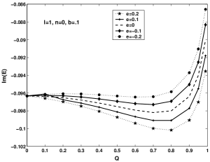
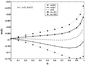
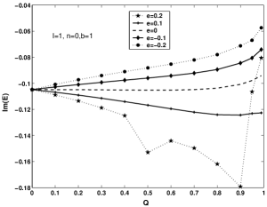
Figure 2: Im(E) vs Q for l=1 and n=0 for each b value(0.1, 0.5 and 1)

Fig.2 shows the behavior of $Im(E)$ versus Q for the mode $l=1$($k=1$) and $n=0$ case. And it is clear that as black hole charge $Q$ increases from 0 to 0.99, at first there is a small increase of $|Im(E)|$ and then it decreases with increase of the charge $Q$. Also for a fixed $b$ value the $|Im(E)|$ is small for negatively charged Dirac field compared to positively charged ones. In $b=0.1$ case that is when the effect of cosmic string is high we get very good curves compared to others. When the $l$ value increases the behavior is similar to the former case. Fig. 3 shows the behavior of $Im(E)$ versus $Q$ for $l=2$ case. Here we considered both the modes $n=1$ and $n=0$ for $b=0.1$ and $b=0.5$. Thus from this we understand that positively charged Dirac field decay faster than negatively charged Dirac field on a positively charged RN black hole with a fixed $b$ value.

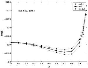
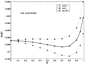
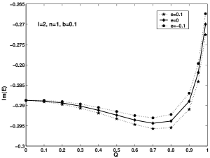
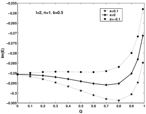
Figure 3: Im(E) vs Q for b=0.1 and 0.5 for l=2, n=0 and n=1

Fig. 4 shows the dependence of $Re(E)$ with black hole charge $Q$ with different values of Dirac field charge $e$ from +0.2 to -0.2 for fixed values of $b$. For all $b$ values $Re(E)$ is increasing with respect to $Q$. From the Fig.4 it is clear that $e=-0.2$ have higher $Re(E)$ compared to $e=0.2$ which implies that negatively charged Dirac field have larger $Re(E)$ value.

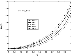
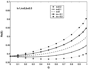
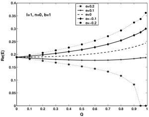
Figure 4: Re(E) vs Q for l=1 and n=0 for fixed values of b(0.1, 0.5, 1)

We now check for the imprint of cosmic string on the RN black hole. For this we plot $Im(E)$ versus $Q$ graph for various $b$ values for a fixed field charge $e$ as in Fig.5. Thus for the mode $l=1$, $n=0$ and when charge of the Dirac field is $e=0.2$, as $Q$ increases, $|Im(E)|$ at first increases and then decreases. But when $b=0.1$ the $|Im(E)|$ is smaller compared to others. i.e., decay is small in the case of black hole having cosmic string. This is true only for the positively charged Dirac field and for $e=0$. When $e$ becomes negative, it shows another behavior. i.e., for the negatively charged Dirac field, up to some $Q$ value (let it be $Q_{0}$) $|Im(E)|$ for $b=0.1$ is small compared to others. The $|Im(E)|$ for $b=0.1,0.5$ and $1$ meets near $Q_{0}$. After that $|Im(E)|$ values for $b=0.1$ become larger than all others. i.e., up to $Q_{0}$ the decay rate is small for a black hole having cosmic string and then decay rate increases.

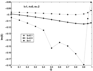
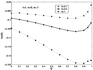
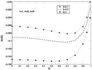
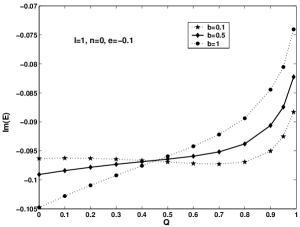
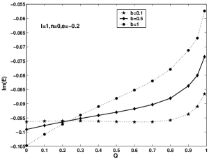
Figure 5: Im(E) vs Q for l=1, n=0 for different e(+2 to -2)values

The variation of $b$ with $e$ values for higher modes (for $l=2$, $n=1$ and $n=2$) are shown in Fig. 6 and Fig. 7. Here also $|Im(E)|$ behaves same as above. i.e, in the case of negatively charged Dirac field, when the charge of the black hole is high, the effect due to cosmic string is suppressed.

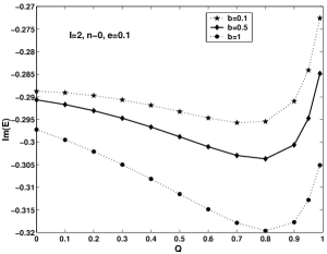
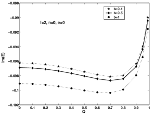
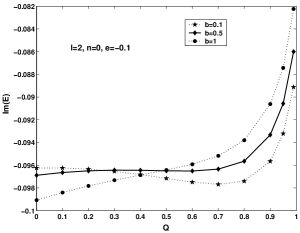
Figure 6: Im(E) vs Q for l=2, n=0 for different e(+1 to -1)values

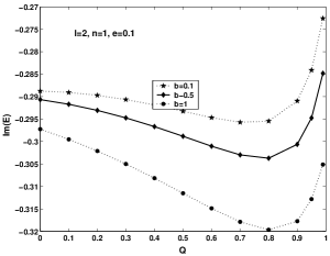
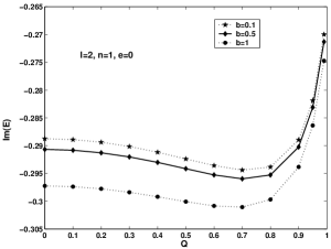
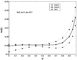
Figure 7: Im(E) vs Q for l=2, n=1 for different e(+1 to -1)values

Fig. 8 shows the variation of $Re(E)$ with $Q$ for various values of $b$ for a fixed $e$. Here for all values of $e$, $Re(E)$ is larger for $b=0.1$ compared to others. That is, $Re(E)$ is larger for the black hole having cosmic string.

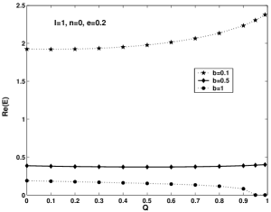
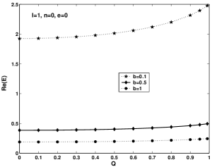
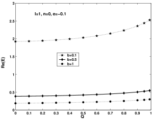
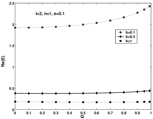
Figure 8: Re(E) vs Q for e=+2, 0, -1 for l=1, and the last one is for l=2

4 Conclusion

We have obtained the Dirac equation in RN black hole space time with a cosmic sting and its deduction into a set of second order differential equations. We have evaluated the quasinormal mode frequencies for RN black hole space times having cosmic string perturbed by a massless Dirac field. We find that for a fixed value of $b$, positively charged Dirac field decay faster than negatively charged Dirac field. But when we compare the RN black hole with and without cosmic string, in the case of positively charged Dirac field, decay is less when cosmic string is present. But in the case of negatively charged Dirac field, the RN black hole having cosmic string shows small decay for low values of black hole charge $Q$ but as $Q$ increases its decay increases. Whereas, the RN black hole which do not have cosmic string shows rapid decay for low values of $Q$ and as $Q$ increases its decay rate decreases compared to the RN black hole having cosmic string. Thus the effect due to cosmic string will dominate only in the case of RN black hole having small charge perturbed by a negatively charged Dirac field.

References

- [1] T. Regge and J. A. Wheeler, Phys. Rev., 108, 1063 (1957).
- [2] C. V. Vishveshwara , Phys. Rev. D, 1, 2870 (1970).
- [3] H. P. Nollert, Class. Quantum. Grav., 16, R159 (1999).
- [4] K. D. Kokkotas and Schmidt B. G., Living Rev. Rel., 2, 2 (1999).
- [5] R. A. Konoplya, Phys. Lett. B, 550, 117 (2002).
- [6] B. Wang, Braz. J. Phys., 35, 1029 (2005).
- [7] A. Vilenkin, Phys. Rep., 121, 263 (1986).
- [8] T. W. B. Kibble, J. Phys. A: Math. Gen., 9, 1387 (1976).
- [9] A. Vilenkin, Phys. Rev. Lett., 46, 1169 (1981); Phys. Rev. D, 24, 2082 (1981).
- [10] T. W. B. Kibble and N. Turok , Phys. Rev. Lett., 116B, 141 (1982).
- [11] A. Vilenkin, Phys. Rev. D 23, 852 (1981).
- [12] S. Chen, B. Wang and R. Su, gr-qc/0701088v1 (2007).
- [13] R. Sini, N. Varghese and V. C. Kuriakose, gr-qc/0802.0788v2 (2008).
- [14] M. Aryal, L. H. Ford and A. Vilenkin, Phys. Rev. D, 34, 2263 (1986).
- [15] D. R. Brill and J. A. Wheeler Revs. Modern. Phys., 29, 465 (1957)
- [16] M.G. Germano, V. B. Bezerra and E. R. Bezerra de Mello, Class. Quantum Grav, 13, 2663 (1996).
- [17] F. Cooper, A. Khare And U. Sukhatme, Phys. Rept., 251, 267 (1995).
- [18] V. Ferrari and B. Mashhoon , Phys. Rev. D, 30, 295 1984.
- [19] Y. J. Wu and Z. Zhao, Phys. Rev. D, 69, 084015(2004).