On adaptive stratification

Abstract

This paper investigates the use of stratified sampling as a variance reduction technique for approximating integrals over large dimensional spaces. The accuracy of this method critically depends on the choice of the space partition, the strata, which should be ideally fitted to the subsets where the functions to integrate is nearly constant, and on the allocation of the number of samples within each strata. When the dimension is large and the function to integrate is complex, finding such partitions and allocating the sample is a highly non-trivial problem. In this work, we investigate a novel method to improve the efficiency of the estimator ”on the fly”, by jointly sampling and adapting the strata which are hyperrectangles and the allocation within the strata. The accuracy of estimators when this method is used is examined in detail, in the so-called asymptotic regime (i.e.  when both the number of samples and the number of strata are large). It turns out that the limiting variance depends on the directions defining the hyperrectangles but not on the precise abscissae of their boundaries along these directions, which gives a mathematical justification to the common choice of equiprobable strata. So, only the directions are adaptively modified by our algorithm. We illustrate the use of the method for the computation of the price of path-dependent options in models with both constant and stochastic volatility. The use of this adaptive technique yields variance reduction by factors sometimes larger than 1000 compared to classical Monte Carlo estimators.

1 Introduction

A number of problems in statistics, operation research and mathematical finance boils down to the evaluation of the expectation (or higher order moments) of a random variable $\phi(Y)$, known to be a complicated real valued function of a vector $Y=(Y_{1},\dots,Y_{d})$ of independent random variables. In our applications, we will mainly focus on simulations driven by a sequence of independent standard normal random variables, in situations where the dimension $d$ is very large. Such problems arise in particular in computational finance for the pricing of path-dependent options, either when the number of underlying assets is large, or when additional source of randomness is present such as in stochastic volatility models.

The stratification approach consists in dissecting $\mathbb{R}^{d}$ into mutually exclusive strata and ensuring that $\phi$ is evaluated for a prescribed and appropriate number of points in each stratum (see glasserman:2004 , asmussen:glynn:2007 , rubinstein:kroese:2008 ).

The main purpose of this paper is to discuss a way of dissecting the space into strata and allocating the random draws in the strata, adapted to the case where $Y$ is a standard Gaussian vector. We also address the accuracy of estimators when this method of sampling is used, and give conditions upon which the variance reduction is most effective.

Our method makes use of orthogonal directions, to induce a dissection of $\mathbb{R}^{d}$ with the right property. These directions and the associated allocation are learnt adaptively, while the simulations are performed. The advantage of the adaptive method, similar to those introduced for importance sampling by rubinstein:kroese:2004 is that information is collected as the simulations are done, and computations of means and variances of $\phi(Y)$ in strata are used to update the choice of these strata and of the allocation. We investigate in some details the asymptotic regime i.e.  where the number of simulations and the number of the strata both go to infinity.

The method is illustrated for pricing path-dependent options driven by high-dimensional Gaussian vectors, combining importance sampling based on a change of drift together with the suggested adaptive stratification. The combination of these two methods, already advocated in an earlier work by glasserman:heidelberger:shahabuddin:1999 , is very effective; nevertheless, these examples show that, contrary to what is suggested in this work, the asymptotical optimal drift vector is not always the most effective direction of stratification.

The paper is organized as follows. In section 2, an introduction to the main ideas of the stratification is presented. Section 3 addresses the behavior of the stratified estimator in the asymptotic regime (i.e.  when both the number of samples and the number of strata go to infinity). The roles of the stratification directions, of the strata boundaries in each direction of stratification and of the allocation within each strata are evidenced. In section 4, an algorithm is proposed to adapt the directions of stratification and the allocation of simulations within each stratum. In Section 5, the proposed adaptive stratification procedure is illustrated using applications for the pricing of path-dependent options.

2 An introduction to stratification

Suppose we want to compute an expectation of the form $\operatorname{E}\left[\phi(Y)\right]$ where $\phi:\mathbb{R}^{d}\to\mathbb{R}$ is a measurable function and $Y$ is a $\mathbb{R}^{d}$-valued random variable. We assume hereafter that

$$\operatorname{E}\left[\phi^{2}(Y)\right]<+\infty\;.$$ (1)

We consider a stratification variable of the form $\mu^{T}Y$ where $\mu$ is an orthonormal $(d\times m)$ matrix with $m\leq d$. Given a finite partition $\left\{\mathsf{S}_{\mathbf{i}},\mathbf{i}\in\mathcal{I}\right\}$ of $\mathbb{R}^{m}$, the sample space $\mathbb{R}^{d}$ of $Y$ is divided into strata defined by

$$\mathsf{S}_{\mu,\mathbf{i}}\stackrel{{\scriptstyle\mathrm{def}}}{{=}}\left\{x\in\mathbb{R}^{d},\mu^{T}x\in\mathsf{S}_{\mathbf{i}}\right\}\;,\quad\mathbf{i}\in\mathcal{I}\;.$$ (2)

It is assumed in the sequel that the probability of the strata $\{p_{\mathbf{i}},\mathbf{i}\in\mathcal{I}\}$

$$p_{\mathbf{i}}(\mu)\stackrel{{\scriptstyle\mathrm{def}}}{{=}}\mathbb{P}\left(Y\in\mathsf{S}_{\mu,\mathbf{i}}\right)=\mathbb{P}\left(\mu^{T}Y\in\mathsf{S}_{\mathbf{i}}\right)\;,$$ (3)

are known which is the case when $Y$ is a standard Gaussian vector and the $S_{\mathbf{i}}$ are hyperrectangles. Up to removing some strata, we may assume without loss of generality that $p_{\mathbf{i}}(\mu)>0$, for any $\mathbf{i}\in\mathcal{I}$.

Let $M$ be the total number of draws and $\mathcal{Q}=\{q_{\mathbf{i}},\mathbf{i}\in\mathcal{I}\}$ be an allocation vector (i.e. $q_{\mathbf{i}}\geq 0$ and $\sum_{\mathbf{i}\in\mathcal{I}}q_{\mathbf{i}}=1$) : the number $M_{\mathbf{i}}$ of samples allocated to the $\mathbf{i}$-th stratum is given by

$$M_{\mathbf{i}}\stackrel{{\scriptstyle\mathrm{def}}}{{=}}\left\lfloor M\sum_{\mathbf{j}\leq\mathbf{i}}q_{\mathbf{j}}\right\rfloor-\left\lfloor M\sum_{\mathbf{j}<\mathbf{i}}q_{\mathbf{j}}\right\rfloor\;,\quad\mathbf{i}\in\mathcal{I}\;,$$ (4)

where $\lfloor\cdot\rfloor$ denotes the lower integer part and by convention, $\sum_{\emptyset}q_{\mathbf{j}}=0$ (it is assumed that the set of indices $\mathcal{I}$ is totally ordered). If the number of points in each stratum is chosen to be proportional to the probability of the strata, the allocation is said to be proportional. Given the strata $\{\mathsf{S}_{\mathbf{i}},\mathbf{i}\in\mathcal{I}\}$ and the allocation $\mathcal{Q}$, the stratified estimator with $M$ draws is defined by

$$\sum_{\mathbf{i}\in\mathcal{I}:M_{\mathbf{i}}>0}p_{\mathbf{i}}(\mu)\left\{\frac{1}{M_{\mathbf{i}}}\sum_{j=1}^{M_{\mathbf{i}}}\phi(Y_{\mathbf{i},j})\right\}\;,$$ (5)

where $\{Y_{\mathbf{i},j},j\leq M_{\mathbf{i}},\mathbf{i}\in\mathcal{I}\}$ are independent random variables with $Y_{\mathbf{i},j}$ distributed according to the conditional distribution $\operatorname{P}\left[\left.Y\in\cdot\,\right|\mu^{T}Y\in\mathsf{S}_{\mathbf{i}}\right]$ for $j\leq M_{\mathbf{i}}$.

The stratified estimator is an unbiased estimator of $\operatorname{E}[\phi(Y)]$ if the $M_{\mathbf{i}}$’s are all positive (a sufficient condition is $M\geq 1/\min_{\mathbf{i}}q_{\mathbf{i}}$). Its variance is given by $\sum_{\mathbf{i}\in\mathcal{I}:M_{\mathbf{i}}>0}\ M_{\mathbf{i}}^{-1}p_{\mathbf{i}}^{2}(\mu)\sigma_{\mathbf{i}}^{2}(\mu)$ where $\sigma_{\mathbf{i}}^{2}(\mu)$ is the conditional variance of the random vector $\phi(Y)$ given $\mu^{T}Y\in\mathsf{S}_{\mathbf{i}}$,

$$\sigma_{\mathbf{i}}^{2}(\mu)\stackrel{{\scriptstyle\mathrm{def}}}{{=}}\operatorname{E}\left[\left.\phi^{2}(Y)\,\right|\mu^{T}Y\in\mathsf{S}_{\mathbf{i}}\right]-\left(\operatorname{E}\left[\left.\phi(Y)\,\right|\mu^{T}Y\in\mathsf{S}_{\mathbf{i}}\right]\right)^{2}\;.$$ (6)

When $M$ goes to infinity and the number of strata is either fixed or goes to infinity slowly enough, the variance of the stratified estimator is equivalent to $M^{-1}\sum_{\mathbf{i}\in\mathcal{I}:q_{\mathbf{i}}>0}\ q_{\mathbf{i}}^{-1}\ p_{\mathbf{i}}^{2}(\mu)\sigma_{\mathbf{i}}^{2}(\mu)$ (see Lemma 1). The two key questions that arise in every application of the stratified sampling method are (i) the choice of the dissection of the space and (ii) for a fixed $M$, the determination of the number of samples $M_{\mathbf{i}}$ to be generated in each stratum $\mathbf{i}$. The optimal allocation minimizing the above asymptotic variance subject to the constraint $\sum_{\mathbf{i}\in\mathcal{I}}q_{\mathbf{i}}=1$ is given by :

$$q^{\star}_{\mathbf{i}}(\mu)\stackrel{{\scriptstyle\mathrm{def}}}{{=}}\frac{p_{\mathbf{i}}(\mu)\;\sigma_{\mathbf{i}}(\mu)}{\sum_{\mathbf{j}\in\mathcal{I}}p_{\mathbf{j}}(\mu)\sigma_{\mathbf{j}}(\mu)}\;.$$ (7)

For a given stratification matrix $\mu$, we refer to $\mathcal{Q}^{\star}(\mu)=\{q^{\star}_{\mathbf{i}}(\mu),\mathbf{i}\in\mathcal{I}\}$ as the optimal stratification vector. Of course, contrary to the proportions $p_{\mathbf{i}}(\mu)$, the conditional expectations $\operatorname{E}\left[\left.\phi(Y)\,\right|Y\in\mathsf{S}_{\mu,\mathbf{i}}\right]$ are unknown and so are the conditional variances $\sigma_{\mathbf{i}}^{2}(\mu)$.

The simplest approach would be to estimate these conditional variances in a pilot run, to determine the optimal stratification matrix and the optimal allocation vector from these estimates, and then to use them in a second stage to determine the stratified estimator. Such a procedure is clearly suboptimal, since the results obtained in the pilot step are not fully exploited. This calls for a more sophisticated procedure, in the spirit of those used for adaptive importance sampling; see for example, rubinstein:kroese:2004 and rubinstein:kroese:2008 . In these algorithms, the estimate of conditional variance and the stratification directions is gradually improved while computing the stratified estimator and estimating its variance. Such algorithm extends the procedure by etore:jourdain:2007 , who proposed to adaptively learn the optimal allocation vector for a set of given strata and derived a central limit theorem for the adaptive estimator (with the optimal asymptotic variance).

3 Asymptotic analysis of the stratification performance

We derive in this Section the asymptotic variance of the stratified estimator when both the total number of draws $M$ and the number of strata (possibly depending upon $M$) tend to $+\infty$. The variance of the estimator depends on the stratification matrix $\mu$, on the partition $\{\mathsf{S}_{\mathbf{i}},\mathbf{i}\in\mathcal{I}\}$ of the sample space of $\mu^{T}Y$ and on the allocation $\mathcal{Q}$.

For any integer $k$, we denote by $\lambda$ the Lebesgue measure on $\mathbb{R}^{k}$, equipped with its Borel sigma-field (the dependence in the dimension $k$ is implicit). For a probability density $h$ w.r.t the Lebesgue measure on $\mathbb{R}$, we denote by $H$ its cumulative distribution function, and $H^{-1}$ its quantile function, defined as the generalized inverse of $H$,

$$H^{-1}(u)=\inf\{x\in\{H>0\}:H(x)\geq u\}\;,\quad\text{for any $u\in[0,1]$}\;,$$

where, by convention, $\inf\emptyset=+\infty$. Let $I$ be a positive integer. The choice of the strata boundaries is parameterized by an $m$-uplet $(g_{1},\dots,g_{m})$ of probability densities on $\mathbb{R}$ in the following sense: for all $m$-uplet $\mathbf{i}=(i_{1},\dots,i_{m})\in\{1,\cdots,I\}^{m}$,

$$\mathsf{S}_{\mathbf{i}}\stackrel{{\scriptstyle\mathrm{def}}}{{=}}\prod_{k=1}^{m}\left(G_{k}^{-1}\left(\frac{i_{k}-1}{I}\right),G_{k}^{-1}\left(\frac{i_{k}}{I}\right)\right]\;.$$ (8)

We denote by $g(x_{1},\dots,x_{m})\stackrel{{\scriptstyle\mathrm{def}}}{{=}}\prod_{k=1}^{m}g_{k}(x_{k})$ the associated joint density. Let $\mu$ be a $d\times m$ orthonormal matrix. We consider the stratification $\mathcal{S}(\mu)=\left\{\mathsf{S}_{\mu,\mathbf{i}},\mathbf{i}\in\{1,\dots,I\}^{m}\right\}$ of the space $\mathbb{R}^{d}$. Denote by $\varsigma^{2}_{I,M}(\mu,g,\mathcal{Q})$ the asymptotic variance of the stratified estimator, given by

$$\varsigma^{2}_{I,M}(\mu,g,\mathcal{Q})\stackrel{{\scriptstyle\mathrm{def}}}{{=}}\sum_{\mathbf{i}\in\{1,\dots,I\}^{m}:M_{\mathbf{i}}>0}M_{\mathbf{i}}^{-1}\ p_{\mathbf{i}}^{2}(\mu)\sigma_{\mathbf{i}}^{2}(\mu)\;,$$ (9)

where the number of draws $M_{\mathbf{i}}$ is given by (4) and $p_{\mathbf{i}}(\mu),\sigma^{2}_{\mathbf{i}}(\mu)$, the probability and the conditional variance are given by (3), and (6), respectively. The dependence w.r.t. $g$ and $\mathcal{Q}$ of $M_{\mathbf{i}}$, $p_{\mathbf{i}}(\mu)$ and $\sigma^{2}_{\mathbf{i}}(\mu)$ is implicit.

We consider allocation vectors $\mathcal{Q}_{\chi}=\left\{q_{\mathbf{i}}(\chi)\stackrel{{\scriptstyle\mathrm{def}}}{{=}}\int_{\mathsf{S}_{\mathbf{i}}}\chi\ d\lambda\;,\mathbf{i}\in\{1,\dots,I\}^{m}\right\}$ parameterized by a probability density $\chi:\mathbb{R}^{m}\to\mathbb{R}_{+}$. We assume that the random variable $\mu^{T}Y$ possesses a density $f_{\mu}$ w.r.t. the Lebesgue measure (on $\mathbb{R}^{m}$). We consider the functions

$$\psi_{\mu}(x)\stackrel{{\scriptstyle\mathrm{def}}}{{=}}\operatorname{E}\left[\left.\phi^{\phantom{2}}(Y)\,\right|\mu^{T}Y=x\right]\;,\quad\text{and}\quad\zeta_{\mu}(x)\stackrel{{\scriptstyle\mathrm{def}}}{{=}}\operatorname{E}\left[\left.\phi^{2}(Y)\,\right|\mu^{T}Y=x\right]\;.$$

Using these notations, the asymptotic variance of the stratified estimator may be rewritten as

$$\varsigma^{2}_{I,M}(\mu,g,\mathcal{Q}_{\chi})=\sum_{\mathbf{i}\in\{1,\dots,I\}^{m}:M_{\mathbf{i}}>0}M_{\mathbf{i}}^{-1}\ \left\{\left(\int_{\mathsf{S}_{\mathbf{i}}}f_{\mu}\ d\lambda\right)\left(\int_{\mathsf{S}_{\mathbf{i}}}\zeta_{\mu}f_{\mu}\ d\lambda\right)-\left(\int_{\mathsf{S}_{\mathbf{i}}}\psi_{\mu}f_{\mu}\ d\lambda\right)^{2}\right\}\;.$$

We will investigate the limiting behavior of asymptotic variance $\varsigma^{2}_{I,M}(\mu,g,\mathcal{Q}_{\chi})$ when the total number of samples $M$ and the number of strata $I$ both tend to $+\infty$. For that purpose, some technical conditions are required. For $\nu$ a measure on $\mathbb{R}^{m}$ and $h$ a real-valued measurable function on $\mathbb{R}^{m}$, we denote by $\mathop{\mathrm{essinf}}_{\nu}\left(h\right)$ and $\mathop{\mathrm{esssup}}_{\nu}\left(h\right)$ the essential infimum and supremum w.r.t. the measure $\nu$. From now on we use the following convention : $z/0$ is equal to $+\infty$ if $z>0$ and to $0$ if $z=0$.

• $\int_{\mathbb{R}^{m}}\chi^{2}/g\,d\lambda<+\infty$ and $\mathop{\mathrm{essinf}}_{g\cdot\lambda}\left(\chi/g\right)>0$.

• for $h\in\{f_{\mu},\zeta_{\mu}f_{\mu},\psi_{\mu}f_{\mu}\}$, $\int_{\mathbb{R}^{m}}h^{2}/g\ d\lambda<+\infty$.

Under A2, $\lambda$-a.e. , $g=0$ implies that $f_{\mu}=0$. Finally, a reinforced integrability condition is needed

• $\int_{\mathbb{R}^{m}}\ f_{\mu}^{4}(\zeta_{\mu}-\psi_{\mu}^{2})^{2}/[\chi^{2}g]\ d\lambda<+\infty$.

When $m<d$, we establish the expression of the limit as the number of strata $I$ goes to $+\infty$ of the limiting variance (as the number of simulations $M$ goes to $+\infty$) of the stratified estimator. Define

$$\varsigma_{\infty}^{2}(\mu,\chi)\stackrel{{\scriptstyle\mathrm{def}}}{{=}}\int_{\mathbb{R}^{m}}f_{\mu}^{2}(\zeta_{\mu}-\psi_{\mu}^{2})/\chi\ d\lambda\;.$$ (10)

Proposition 1

Let $m$ be an integer such that $m<d$, $g_{1},\cdots,g_{m}$ be probability density functions (pdf) w.r.t. to the Lebesgue measure of $\mathbb{R}$, $\mu$ be a $d\times m$ orthonormal matrix, and $\chi$ be a pdf w.r.t. the Lebesgue measure on $\mathbb{R}^{m}$. Assume that $g$ and $\chi$ satisfy assumptions A1-A3. Then

$$\lim_{I\to+\infty}\lim_{M\to+\infty}M\varsigma_{I,M}^{2}(\mu,g,\mathcal{Q}_{\chi})=\varsigma^{2}_{\infty}(\mu,\chi)\;.$$

Assume in addition one of the following conditions

1. $\mathop{\mathrm{esssup}}_{\chi\cdot\lambda}\left(f_{\mu}/\chi\right)<+\infty$ and $\{I_{M},M\geq 1\}$ is an integer-valued sequence such that $I_{M}^{-1}+I^{m}_{M}M^{-1}\to 0$ as $M$ goes to infinity.

2. $\{I_{M},M\geq 1\}$ is an integer-valued sequence such that $I_{M}^{-1}+I^{2m}_{M}M^{-1}\to 0$ as $M$ goes to infinity.

Then,

$$\lim_{M\to+\infty}M\varsigma_{I_{M},M}^{2}(\mu,g,\mathcal{Q}_{\chi})=\varsigma_{\infty}^{2}(\mu,\chi)\;.$$

The proof is given in Section 6.1. It is worthwhile to note that the limiting variance of the stratified estimator $\varsigma_{\infty}^{2}(\mu,\chi)$ does not depend on the densities $(g_{1},\dots,g_{m})$ that define the strata : only the stratification matrix $\mu$ and the allocation vector $\mathcal{Q}_{\chi}$ enters in the limit. The contribution to the variance of the randomness in the directions orthogonal to the rows of $\mu$ dominates at the first order. In practice, this means that asymptotically, once the directions of stratification are chosen, the choice of the strata is irrelevant; the usual choice of $g_{i}$ as the distribution of the $i$-th component of the random vector $\mu^{T}Y$, $i\in\{1,\dots,m\}$ is asymptotically optimal.

On the contrary, the limiting variance $\varsigma_{\infty}^{2}(\mu,\chi)$ depends on the allocation density $\chi$. For a given value of the stratification directions $\mu$, it is possible to minimize the function $\chi\mapsto\varsigma_{\infty}^{2}(\mu,\chi)$. Assume that $\int_{\mathbb{R}^{m}}f_{\mu}\sqrt{\zeta_{\mu}-\psi_{\mu}^{2}}\ d\lambda>0$. Since $\int_{\mathbb{R}^{m}}f_{\mu}\sqrt{\zeta_{\mu}-\psi_{\mu}^{2}}\ d\lambda=\operatorname{E}\left[\sqrt{\mathrm{Var}\left[\phi(Y)|\mu^{T}Y\right]}\right]\leq\sqrt{\mathrm{Var}(\phi(Y))},$ the integral is finite by (1) and it is possible to define a density $\chi_{\mu}^{\star}$ by

$$\chi_{\mu}^{\star}\stackrel{{\scriptstyle\mathrm{def}}}{{=}}f_{\mu}\sqrt{\zeta_{\mu}-\psi_{\mu}^{2}}\bigg{/}\int_{\mathbb{R}^{m}}f_{\mu}\sqrt{\zeta_{\mu}-\psi_{\mu}^{2}}\ d\lambda\;.$$ (11)

Then $\chi_{\mu}^{\star}$ is the minimum of $\chi\mapsto\varsigma_{\infty}^{2}(\mu,\chi)$ and the minimal limiting variance is

$$\varsigma_{\infty}^{2}(\mu,\chi_{\mu}^{\star})=\left(\int_{\mathbb{R}^{m}}f_{\mu}\sqrt{\zeta_{\mu}-\psi_{\mu}^{2}}\ d\lambda\right)^{2}=\left(\operatorname{E}\left[\sqrt{\mathrm{Var}\left[\phi(Y)|\mu^{T}Y\right]}\right]\right)^{2}\;.$$

Provided $\chi_{\mu}^{\star}$ satisfies assumptions A1-2 (note that in that case, A3 is automatically satisfied), the choice $\chi=\chi_{\mu}^{\star}$ for the allocation of the drawings in the strata is asymptotically optimal.

Remark 1

An expression of the limiting variance $\varsigma_{\infty}^{2}(\mu,\chi)$ has been obtained in (glasserman:heidelberger:shahabuddin:1999, , Lemma 4.1) in the case $m=1$ and for the proportional allocation rule which corresponds to $\chi=f_{\mu}$. It is shown by these authors that the limiting variance is $\operatorname{E}\left(\mathrm{Var}\left[\left.\phi(Y)\,\right|\mu^{T}Y\right]\right)$ which is equal to $\varsigma_{\infty}^{2}(\mu,f_{\mu})$ (note that in this case the stratification density $g=f_{\mu}$, satisfies the assumptions A1-3 provided that $\operatorname{E}[\phi^{4}(Y)]<\infty$). Unless $\mathrm{Var}\left[\left.\phi(Y)\,\right|\mu^{T}Y\right]$ is a.s. constant, the asymptotic variance is strictly smaller for the optimal choice of the allocation density.

The optimal allocation density $\chi_{\mu}^{\star}$ cannot in general be computed explicitly but, as shown in the following Proposition, can be approximated by computing the optimal allocation within each stratum.

Proposition 2

Let $m<d$ be an integer and $\mu$ be an $(d\times m)$ orthonormal matrix. Assume that A2 is satisfied. Then,

$$\lim_{I\to+\infty}\sum_{\mathbf{i}\in\{1,\dots,I\}^{m}}\left|q^{\star}_{\mathbf{i}}(\mu)-\int_{\mathsf{S}_{\mathbf{i}}}\chi_{\mu}^{\star}\ d\lambda\right|=0\;,$$

where $\mathcal{Q}^{\star}(\mu)\stackrel{{\scriptstyle\mathrm{def}}}{{=}}\{q^{\star}_{\mathbf{i}}(\mu),\mathbf{i}\in\{1,\dots,I\}^{m}\}$ is given by (7). Let $\{I_{M},M\geq 1\}$ be an integer-valued sequence such that $I_{M}^{-1}+I^{m}_{M}M^{-1}\to 0$ as $M$ goes to infinity. Then,

$$\lim_{M\to+\infty}M\varsigma_{I_{M},M}^{2}(\mu,g,\mathcal{Q}^{\star}(\mu))=\varsigma_{\infty}^{2}(\mu,\chi_{\mu}^{\star})\;.$$

The proof is given in Section 6.1. As the number of strata goes to infinity, the stratified estimator run with the optimal allocation $\mathcal{Q}^{\star}(\mu)$ has the same asymptotic variance as the stratified estimator run with the allocation deduced from the optimal density $\chi_{\mu}^{\star}$. In practice, of course, the optimal allocation $\mathcal{Q}^{\star}(\mu)$ is unknown, but it is possible to construct an estimator of this quantity by estimating the conditional variance of $\mathrm{Var}[\phi(Y)|\mu^{T}Y\in\mathsf{S}_{\mathbf{i}}]$ within each stratum (etore:jourdain:2007, ).

Remark 1

When $m=d$, the results obtained are markedly different since the accuracy of the stratified estimator now depends on the definition of the strata along each direction. Let $\phi_{\mu}(x)\stackrel{{\scriptstyle\mathrm{def}}}{{=}}\phi(\mu^{T}x)$, $\partial_{k}\phi_{\mu}$ be the partial derivative of $\phi_{\mu}$ w.r.t. its $k$-th coordinate for $k\in\{1,\dots,d\}$. Let $g_{k}$ still denote the function $x=(x_{1},\dots,x_{d})\in\mathbb{R}^{d}\mapsto g_{k}(x_{k})$. Assuming A1, $\mathop{\mathrm{esssup}}_{\lambda}\left(f_{\mu}/g\right)<+\infty$ and $\phi\in C^{1}$ satisfies $\mathop{\mathrm{esssup}}_{\lambda}\left(\sum_{k=1}^{d}|\partial_{k}\phi_{\mu}|/g_{k}\right)<+\infty$, one checks in etore:fort:jourdain:moulines:2008 that for any integer-valued sequence $\{I_{M},M\geq 1\}$ such that $\lim_{M\to\infty}\left(I_{M}^{-1}+I^{d+2}_{M}M^{-1}\right)=0$,

$$\lim_{M\to+\infty}MI_{M}^{2}\varsigma_{I_{M},M}^{2}(\mu,g,\mathcal{Q}_{\chi})=\varsigma_{\infty}^{2}(\mu,g,\chi)\stackrel{{\scriptstyle\mathrm{def}}}{{=}}\frac{1}{12}\int_{\mathbb{R}^{d}}\frac{f_{\mu}^{2}}{\chi}\sum_{k=1}^{d}\left(\frac{\partial_{k}\phi_{\mu}}{g_{k}}\right)^{2}d\lambda.$$

In addition, $\lim_{M\to+\infty}MI_{M}^{2}\varsigma_{I_{M},M}^{2}(\mu,g,\mathcal{Q}^{\star}(\mu))=\varsigma_{\infty}^{2}(\mu,g,\chi^{\star}_{\mu,g})$ with $\chi^{\star}_{\mu,g}\propto f_{\mu}\sqrt{\sum_{k=1}^{d}\left(\frac{\partial_{k}\phi_{\mu}}{g_{k}}\right)^{2}}$.

4 An adaptive stratification algorithm

As shown in the asymptotic theory presented above, under optimal allocation, it is more important to optimize the stratification matrix $\mu$ than the strata boundaries along each stratification direction . Proposition 1 suggests the following strategy: the “optimal” matrix $\mu_{\star}$ is defined as a minimizer of the limiting variance $\mu\mapsto\varsigma_{\infty}^{2}(\mu,\chi_{\mu}^{\star})$. Of course, this optimization problem does not have a closed form expression because the functions $x\mapsto\psi_{\mu}(x)$, $x\mapsto\zeta_{\mu}(x)$ are not available.

We rather use the characterization of $\varsigma_{\infty}^{2}(\mu,\chi_{\mu}^{\star})$ as the limiting variance of the stratified estimator with optimal allocation given in Proposition 2. The problem boils down to search for a minimizer $\mu$ of the variance $\varsigma^{2}_{I,M}(\mu,g,\mathcal{Q}^{\star}(\mu))$. In our applications, $Y$ is a $d$-dimensional standard normal vector, and $\mu^{T}Y$ is a $m$-dimensional standard Gaussian vector. In this case, we set $g_{i}$, $i=\{1,\dots,m\}$ to be the standard Gaussian distribution so that the strata boundaries in each directions are the quantiles of the standard normal variable. Since $\varsigma_{\infty}^{2}(\mu,\chi_{\mu}^{\star})$ does not depend on $g$, the impact of this convenient choice, which leads to equiprobable strata for the vector $\mu^{T}Y$, should be limited.

Of course, the optimization of $\varsigma^{2}_{I,M}(\mu,g,\mathcal{Q}^{\star}(\mu))$ is a difficult task because in particular the definition of this function involves multidimensional integrals, which cannot be computed with high accuracy. Note also that, in most situations, the optimization should be done in parallel to the main objective, namely, the estimation of the quantity of interest $\operatorname{E}[\phi(Y)]$, which is obtained using a stratified estimator based on the adaptively defined directions of stratification $\mu$. The adaptive stratification is analog to the popular adaptive importance sampling; see for example rubinstein:kroese:2004 , arouna:2004 , kawai:2007 , and rubinstein:kroese:2008 .

When the function to minimize is an expectation, the classical approaches to tackle this problem are based on Monte Carlo approximations for the integrals appearing in the expression of the objective function and its gradients. There are typically two approaches to Monte Carlo methods, the stochastic approximation procedure and the sample average approximation method; see juditsky:lan:nemirovski:shapiro:2007 . In the adaptive stratification context, these Monte Carlo estimators are based on the current fit of the stratification matrix and of the conditional variances within each stratum, the underlying idea being that the algorithm is able to progressively learn the optimal stratification, while the stratified estimator is constructed.

The algorithm described here is closely related to the sample average approximation method, the main difference with the classical approach being that, at every time a new search direction is computed, a new Monte Carlo sample (using the current fit of the strata and of the allocation) is drawn.

Suppose that $Y$ admits a density w.r.t. the Lebesgue measure denoted by $f$. Define for $\mathbf{i}\in\{1,\cdots,I\}^{m}$, a function $h\in\{f,\phi f,\phi^{2}f\}$ , and an orthonormal $d\times m$ matrix $\mu$,

$$\nu_{\mathbf{i}}(h,\mu)\stackrel{{\scriptstyle\mathrm{def}}}{{=}}\int_{\mathsf{S}_{\mu,\mathbf{i}}}h\ d\lambda=\int\prod_{k=1}^{m}\mathbbm{1}_{\{y,G_{k}^{-1}((\mathbf{i}_{k}-1)/I)\leq\left\langle\mu_{k},y\right\rangle\leq G_{k}^{-1}(\mathbf{i}_{k}/I)\}}h\ d\lambda\;,$$ (12)

where $\left\langle x,y\right\rangle$ denotes the scalar product of the vectors $x$ and $y$ and $\mu_{k}$ the $k$-th column of $\mu$. Using the definition of $\nu_{\mathbf{i}}$, the proportions $p_{\mathbf{i}}(\mu)$ and the conditional variances in each stratum $\sigma_{\mathbf{i}}^{2}(\mu)$ respectively given by (3) and  (6) may be expressed as, when $\nu_{\mathbf{i}}(f,\mu)>0$,

$$p_{\mathbf{i}}(\mu)=\nu_{\mathbf{i}}(f,\mu)\;,\quad\text{and}\quad\sigma_{\mathbf{i}}^{2}(\mu)=\frac{\nu_{\mathbf{i}}(f\phi^{2},\mu)}{\nu_{\mathbf{i}}(f,\mu)}-\left(\frac{\nu_{\mathbf{i}}(f\phi,\mu)}{\nu_{\mathbf{i}}(f,\mu)}\right)^{2}\;.$$ (13)

When $M$ is large and $I$ is fixed, minimizing the asymptotic variance of the stratified estimate with optimal allocation is equivalent to minimize $V(\mu)$ w.r.t. the stratification matrix $\mu$ where (see Lemma 1)

$$V(\mu)\stackrel{{\scriptstyle\mathrm{def}}}{{=}}\sum_{\mathbf{i}=1}^{\mathcal{I}}p_{\mathbf{i}}(\mu)\sigma_{\mathbf{i}}(\mu)=\sum_{\mathbf{i}=1}^{\mathcal{I}}\left(\nu_{\mathbf{i}}(f,\mu)\nu_{\mathbf{i}}(f\phi^{2},\mu)-\nu_{\mathbf{i}}^{2}(f\phi,\mu)\right)^{1/2}\;.$$

Assuming that the functions $\mu\mapsto\nu_{\mathbf{i}}(h,\mu)$ are differentiable at $\mu$ for $h\in\{f,f\phi,f\phi^{2}\}$, the gradient may be expressed as

$$\nabla_{\mu}\;V(\mu)=\sum_{\mathbf{i}=1}^{\mathcal{I}}\frac{\nabla_{\mu}\nu_{\mathbf{i}}(f,\mu)\ \nu_{\mathbf{i}}(f\phi^{2},\mu)+p_{\mathbf{i}}(\mu)\ \nabla_{\mu}\nu_{\mathbf{i}}(f\phi^{2},\mu)-2\nu_{\mathbf{i}}(f\phi,\mu)\ \nabla_{\mu}\nu_{\mathbf{i}}(f\phi,\mu)}{2\ p_{\mathbf{i}}(\mu)\sigma_{\mathbf{i}}(\mu)}\mathbbm{1}_{\{p_{\mathbf{i}}(\mu)\sigma_{\mathbf{i}}(\mu)\neq 0\}}\;.$$ (14)

The computation of this gradient thus requires to calculate $\nabla_{\mu}\,\nu_{\mathbf{i}}(h,\mu)$ for $h\in\{f,f\phi,f\phi^{2}\}$. For a vector $\nu\in\mathbb{R}^{d}$, $\nu\neq 0$, and $z\in\mathbb{R}$, define $\lambda_{z}^{\nu}$, the restriction of the Lebesgue measure on the hyperplane $\{y\in\mathbb{R}^{d},\left\langle\nu,y\right\rangle=z\}$.

Proposition 3

Let $z\in\mathbb{R}$, $h:\mathbb{R}^{d}\rightarrow{\mathbb{R}}$ be a locally bounded integrable real function, $g_{z}:\mathbb{R}^{d}\ni\nu\mapsto\int\mathbbm{1}_{\{y,\left\langle\nu,y\right\rangle\leq z\}}h(y)\ d\lambda(y)\;$ and $\mu\in\mathbb{R}^{d}$ be a non-zero vector. Assume that $h$ is continuous $\lambda_{z}^{\mu}$ almost everywhere and that there exists $\varepsilon>0$ such that

$$\lim_{M\rightarrow+\infty}\sup_{|\nu-\mu|\leq\varepsilon}\int|y|\mathbbm{1}_{\{|y|\geq M\}}|h(y)|\;d\lambda_{z}^{\nu}(y)=0\;.$$ (15)

Then, the function $\nu\mapsto g_{z}(\nu)$ is differentiable at $\mu$ and $\nabla_{\mu}\;g_{z}(\mu)=-\int\frac{y}{|\mu|}\;h(y)\;d\lambda_{z}^{\mu}(y)$.

Corollary 1

Assume that $h$ is a real locally bounded integrable function. Let $m$ be an integer, $z=(z_{1},\dots,z_{m})\in\mathbb{R}^{m}$, $g_{z}:\mathbb{R}^{d\times m}\ni(\nu_{1},\dots,\nu_{m})\mapsto\int\prod_{k=1}^{m}\mathbbm{1}_{\{y,\left\langle\nu_{k},y\right\rangle\leq z_{k}\}}h(y)\ d\lambda(y)$ and $\mu=[\mu_{1},\dots,\mu_{m}]\in\mathbb{R}^{d\times m}$ be a full rank matrix. Assume that $h$ is continuous $\sum_{k=1}^{m}\lambda_{z}^{\mu_{k}}$ almost everywhere and that there exists $\varepsilon>0$ such that, for any $k\in\{1,\dots,m\}$, $\lim_{M\rightarrow+\infty}\sup_{|\nu-\mu_{k}|\leq\varepsilon}\int|y|\mathbbm{1}_{\{|y|\geq M\}}|h(y)|\;d\lambda_{z}^{\nu}(y)=0$. Then, $g_{z}$ is differentiable at $\mu$ and the differential $\nabla_{\mu}g_{z}$ is given by $\nabla_{\mu}g_{z}=[\nabla_{\mu_{1}}g_{z},\dots,\nabla_{\mu_{m}}g_{z}]$, where

$$\nabla_{\mu_{i}}g_{z}(\mu)=-\int\frac{y}{|\mu_{i}|}\;\prod_{k\neq i}\mathbbm{1}_{\{y,\left\langle\mu_{k},y\right\rangle\leq z_{k}\}}h(y)\;d\lambda_{z_{i}}^{\mu_{i}}(y)\;.$$

The algorithm goes as follows. Denote by $\{\gamma_{t}\}$ a sequence of stepsizes. Consider the strata $\{\mathsf{S}_{\mathbf{i}},\mathbf{i}\in\{1,\cdots,I\}^{m}\}$ given by (8) for some product density $g$.

• 1. Initialization. Choose initial stratification directions $\mu^{(0)}$ and an initial number of draws in each statum $M^{(0)}\stackrel{{\scriptstyle\mathrm{def}}}{{=}}\{M_{\mathbf{i}}^{(0)},\mathbf{i}\in\stackrel{{\scriptstyle\mathrm{def}}}{{=}}\{1,\dots,I\}^{m}\}$ such that $\sum_{\mathbf{i}}M_{\mathbf{i}}^{(0)}=M$. Compute the probabilities $p_{\mathbf{i}}(\mu^{(0)})$ of each stratum.

  2. Iteration. At iteration $t+1$, given $\mu^{(t)}$, $M^{(t)}$ and $\{p_{\mathbf{i}}(\mu^{(t)}),\mathbf{i}\in\{1,\cdots,I\}^{m}\}$,

     1. Compute $\widehat{\nabla V}(\mu^{(t)})$:

        1. for $\mathbf{i}\in\{1,\cdots,I\}^{m}$, draw $M_{\mathbf{i}}^{(t)}$ realizations of i.i.d. random variables $\{Y_{\mathbf{i},k}^{(t)},k\leq M_{\mathbf{i}}^{(t)}\}$ with distribution $\mathbb{P}(Y\in\cdot|Y\in\mathsf{S}_{\mu^{(t)},\mathbf{i}})$ and evaluate $\hat{\nu}_{\mathbf{i}}^{(t+1)}(h)=\frac{p_{\mathbf{i}}(\mu^{(t)})}{M_{\mathbf{i}}^{(t)}}\sum_{k=1}^{M_{\mathbf{i}}^{(t)}}\ h\left(Y_{\mathbf{i},k}^{(t)}\right)$ for $h\in\{\phi,\phi^{2}\}$.

        2. for $k\in\{1,\cdots,m\}$, $s\in\{G_{k}^{-1}(1/I),\cdots,G_{k}^{-1}((I-1)/I)\}$, draw $\tilde{M}_{k,s}^{(t)}$ realizations of i.i.d. random variables with distribution $\mathbb{P}(Y\in\cdot|[\mu^{(t)}_{k}]^{T}Y=s)$. Compute a Monte Carlo estimate of $\nabla_{\mu}\nu_{\mathbf{i}}(h,\mu^{(t)})$ for $h\in\{f,f\phi,f\phi^{2}\}$ based on Corollary 1.

        3. Compute a Monte Carlo estimate of $\nabla V(\mu^{(t)})$ based on the expression (14).

     2. Update the direction of stratification: Set $\tilde{\mu}=\mu^{(t)}-\gamma_{t}\ \widehat{\nabla V}(\mu^{(t)})$; define $\mu^{(t+1)}$ as the orthonormal matrix found by computing the singular value decomposition of $\tilde{\mu}$ and keeping the $m$ left singular vectors.

     3. Update the allocation policy:

        1. compute an estimate $\hat{\sigma}_{\mathbf{i}}^{(t+1)}$ of the standard deviation within stratum $\mathbf{i}$

           $$\hat{\sigma}_{\mathbf{i}}^{(t+1)}=\left(\frac{\hat{\nu}_{\mathbf{i}}^{(t+1)}(\phi^{2})}{p_{\mathbf{i}}(\mu^{(t)})}-\left(\frac{\hat{\nu}_{\mathbf{i}}^{(t+1)}(\phi)}{p_{\mathbf{i}}(\mu^{(t)})}\right)^{2}\right)^{1/2}\;.$$

        2. Update the allocation vector

           $$q_{\mathbf{i}}^{(t+1)}=\frac{p_{\mathbf{i}}(\mu^{(t)})\ \hat{\sigma}_{\mathbf{i}}^{(t+1)}}{\sum_{\mathbf{j}\in\{1,\dots,I\}^{m}}p_{\mathbf{j}}(\mu^{(t)})\ \hat{\sigma}_{\mathbf{j}}^{(t+1)}}\;,$$

           and the number of draws $\{M_{\mathbf{i}}^{(t+1)},\mathbf{i}\in\{1,\dots,I\}^{m}\}$ by applying the formula (4) with a total number of draws equal to $M$.

     4. Update the probabilities $p_{\mathbf{i}}(\mu^{(t+1)})$, $\mathbf{i}\in\{1,\cdots,I\}^{m}$.

     5. Compute an averaged stratified estimate of the quantity of interest: Estimate the Monte Carlo variance of the stratified estimator for the current fit of the strata and the optimal allocation

        $$[\varsigma^{2}]^{(t+1)}=\frac{1}{M}\left(\sum_{\mathbf{i}\in\{1,\cdots,I\}^{m}}p_{\mathbf{i}}(\mu^{(t)})\ \hat{\sigma}_{\mathbf{i}}^{(t+1)}\right)^{2}\;.$$

        Compute the current fit of the stratified estimator by the following weighted average

        $$\mathcal{E}^{(t+1)}=\left(\sum_{\tau=1}^{t+1}\frac{1}{[\varsigma^{2}]^{(\tau)}}\right)^{-1}\ \sum_{\tau=1}^{t+1}\frac{1}{[\varsigma^{2}]^{(\tau)}}\sum_{\mathbf{i}\in\{1,\cdots,I\}^{m}}\hat{\nu}_{\mathbf{i}}^{(\tau)}(\phi)\;.$$ (16)

There are two options to choose the stepsizes $\{\gamma_{t},t\geq 0\}$. The traditional approach consists in taking a decreasing sequence satisfying the following conditions (see for example pflug:1996 ; kushner:yin:2003 )

$$\sum_{t\geq 0}\gamma_{t}=+\infty\;,\qquad\qquad\sum_{t\geq 0}\gamma_{t}^{2}<+\infty\;.$$

If the number of simulations is fixed in advance, say equal to $N$, then one can use a constant stepsize strategy, i.e.  choose $\gamma_{t}=\gamma$ for all $t\in\{1,\dots,N\}$. As advocated in juditsky:lan:nemirovski:shapiro:2007 , a sensible choice in this setting is to take $\gamma_{t}$ proportional to $N^{-1/2}$. The convergence of this crude gradient algorithm proved to be quite fast in all our applications, so it is not required to resort to computationally involved alternatives.

Step 2(a)ii is specific to the optimization problem to solve and is not related to the stratification itself. The number of draws for the computation of the surface integral (see Corollary 1) can be chosen independently of the allocation $M^{(t)}$. When the samples in steps 2(a)i and 2(a)ii can be obtained by transforming the same set of variables (see Section 5 for such a situation), it is natural to choose $\tilde{M}^{(t)}=\{\tilde{M}_{k,s}^{(t)},k\in\{1,\cdots,m\},s\in\{G_{k}^{-1}(1/I),\cdots,G_{k}^{-1}((I-1)/I)\}\}$ such that $\sum_{k,s}\tilde{M}_{k,s}^{(t)}=M$.

When $f_{\mu}$ has a product form (which is the case e.g. when $Y$ is a standard d-dimensional Gaussian distribution), we can set $g=f_{\mu}$. Then, the strata are equiprobable and $p_{\mathbf{i}}(\mu)=1/I^{m}$ for any ($\mathbf{i}$, $\mu$).

It is out of the scope of this paper to prove the convergence of this algorithm and we refer the reader to classical treatises on this subject. The above algorithm provides, at convergence, both (i) “optimal” directions of stratification and an estimate of the associated optimal allocation; (ii) an averaged stratified estimate $\mathcal{E}$. By omitting the step 2e, the algorithm might be seen as a mean for computing the stratification directions and the associated optimal allocation, and these quantities can then be plugged in a “usual” stratification procedure.

5 Applications in Financial Engineering

The pricing of an option amounts to compute the expectation $\operatorname{E}\left[\Xi(Y)\right]$ for some measurable non-negative function $\Xi$ on $\mathbb{R}^{d}$, where $Y$ is a standard $d$-multivariate Gaussian variable. The Cameron-Martin formula implies that for any $\nu\in\mathbb{R}^{d}$,

$$\operatorname{E}\left[\Xi(Y)\right]=\operatorname{E}\left[\Xi(Y+\nu)\ \exp(-\nu^{T}Y-0.5\nu^{T}\nu)\right]\;,$$ (17)

The variance of the plain Monte Carlo estimator depends on the choice of $\nu$. In all the experiments below (except for the glasserman:heidelberger:shahabuddin:1999 estimator), we use either $\phi(y)=\Xi(y)$ (case $\nu=0$) or $\phi(y)=\Xi(y+\nu_{\star})\ \exp(-\nu^{T}_{\star}y-0.5\nu^{T}_{\star}\nu_{\star})$ where $\nu_{\star}$ is the solution of the optimization problem

$$\mathrm{argmax}_{\{\nu\in\mathbb{R}^{d},\Xi(\nu)>0\}}\ \ \left\{\ln\Xi(\nu)-0.5\nu^{T}\nu\right\}\;,$$ (18)

(case $\nu=\nu_{\star}$). The motivations for this particular choice of the drift vector $\nu$ and procedures to solve this optimization problem are discussed in glasserman:heidelberger:shahabuddin:1999 .

We apply the adaptive stratification procedure introduced in Section 4 (hereafter referred to as “AdaptStr”) in the case $m=1$. For comparison purposes, we also run the stratification procedure proposed in glasserman:heidelberger:shahabuddin:1999 (hereafter referred to as “ GHS”), combining (i) importance sampling with the drift $\nu_{\star}$ defined in (18), and (ii) stratification with proportional allocation and direction $\mu_{\mathsf{g}}$ defined in (glasserman:heidelberger:shahabuddin:1999, , Section 4.2).

We also run stratification algorithms with three different directions of stratification: the vector $\mu_{\star}\propto\nu_{\star}$, the vector $\mu_{\mathrm{reg}}$ proportional to the vector of linear regression of the function $\phi(Y)$ on $Y$ (these regression coefficients are obtained in a pilot run), and a vector $\mu_{l}$ which is a simple guess specific to each application. For these three directions, we run stratification with proportional allocation (case “$q_{i}$” set to “prop”) and with optimal allocation (case “$q_{i}$” set to “opt”). We also run the plain Monte Carlo estimator (column “MC”); when used with $\nu=\nu_{\star}$, ”MC” corresponds to an importance sampling estimator with a drift function $\nu_{\star}$.

Finally, we compare these stratified estimators to Latin Hypercube (LH) estimators (see glasserman:2004 , owen:2003 for a description of this method). For $Y$ a standard normal vector in $\mathbb{R}^{d}$, the expectation of interest $\operatorname{E}[\phi(Y)]$ is also equal to $\operatorname{E}[\phi(OY)]$ for any orthogonal matrix $O\in\mathbb{R}^{d\times d}$ but the variance of the LH estimator associated with the variable $\phi(OY)$ depends on the choice of $O$. Unfortunately, it is very difficult to compute explicitly the asymptotic variance of LH estimators and therefore to adapt the matrix $O$; see owen:1992 . Since LH somehow consists in stratifying each canonical direction, choosing the first column of $O$ equal to the stratification direction $\mu$ should be sensible. In our numerical experiments, we consider such matrices $O$ obtained by orthonormalization of the basis combining $\mu$ and the $d-1$ last vectors of the canonical basis of ${\mathbb{R}}^{d}$ with $\mu$ equal to $\mu_{\star}$, $\mu_{\mathrm{reg}}$ or to the adaptive stratification direction obtained by our algorithm AdaptStr.

5.1 Practical implementations of the adaptive stratification procedure

The numerical results have been obtained by running Matlab codes available from the authors In the numerical applications below, $m=1$. We choose $g=f_{\mu}$ so that the strata are equiprobable ($p_{\mathbf{i}}(\mu)=1/I$). We choose $I=100$ strata and $M=20\,000$ draws per iterations.

The drift vector $\nu$ that solves (18) is obtained by running solnp, a nonlinear optimization program in Matlab freely available at http://www.stanford.edu/$\sim$yyye/matlab/. The direction $\mu^{(0)}$ is set to the unitary constant vector $(1,\cdots,1)/\sqrt{d}$; the initial allocation $M^{(0)}$ is proportional. Exact sampling under the conditional distributions $\mathbb{P}(Y\in\cdot|Y\in\mathsf{S}_{\mu^{(t)},\mathbf{i}})$ and $\mathbb{P}(Y\in\cdot|[\mu^{(t)}]^{T}Y=s)$ can be done by linear transformation of standard Gaussian vectors (see (glasserman:2004, , section 4.3, p. 223)). The draws in step 2(a)i and 2(a)ii can be obtained by transforming the same set of $M^{(t)}$ Gaussian random variables $\{V^{\mathbf{i}}_{j},j\leq M_{\mathbf{i}}^{(t)},\mathbf{i}\in\{1,\cdots,I\}\}$. Therefore, the total number of $d$-dimensional Gaussian draws by iteration is $M$ (the estimates of $\nu_{\mathbf{i}}(h,\mu)$ and $\nabla_{\mu}\nu_{\mathbf{i}}(h,\mu)$ are not independent); $M$ uniform draws in $(0,1)$ are also required to sample under the conditional distribution $\mathbb{P}(Y\in\cdot|Y\in\mathsf{S}_{\mu^{(t)},\mathbf{i}})$. The criterion is optimized using a fixed stepsize steepest descent algorithm (the stepsize is determined using a limited set of pilot runs).

5.2 Assessing efficiency of the adaptive stratification procedure

We compare the averaged stratified estimate $\mathcal{E}^{(N)}$ obtained after $N=200$ iterations, with different stratification procedures and with the crude Monte Carlo estimate. We report in the tables below the estimate of the option prices and the estimates of the variance of the estimator obtained from 50 independent replications.

The comparison of the procedures relies on the variance of the estimators. The column “MC” is an estimate of the variance of $\phi(Y)$ computed with $MN$ i.i.d. samples of a $d$-multivariate gaussian distribution. In the case $\nu=0$, this is an estimation of the variance of the plain Monte Carlo estimator; when $\nu=\nu_{\star}$, this corresponds to an estimation of the Importance Sampling estimator (with importance sampling distribution equal to a standard Gaussian distribution centered at $\nu_{\star}$). The column “AdaptStr” is the limiting variance per sample of $\mathcal{E}^{(N)}$ which is equal to

$$N\,\left\{\sum_{t=1}^{N}\left(\left[\sum_{\mathbf{i}}p_{\mathbf{i}}\,\hat{\sigma}_{\mathbf{i}}^{(t)}\right]^{2}\right)^{-1}\right\}^{-1}\sim\left(\sum_{\mathbf{i}}p_{\mathbf{i}}\,\sigma_{\mathbf{i}}(\mu^{(+\infty)})\right)^{2}\;,$$

when each iteration $t\in\{1,\cdots,N\}$ implies $M$ draws (see the algorithm in Section 4); note that by definition of our procedure, the allocation is optimal. The column “GHS” is an estimate of $\sum_{\mathbf{i}}p_{\mathbf{i}}\sigma_{\mathbf{i}}^{2}(\mu_{\mathsf{g}})$ computed with $MN$ samples; note also that by definition of this procedure, only the case $\nu=\nu_{\star}$ and the proportional allocation has been considered. The columns “$\mu_{\mathrm{reg}}$”, “$\mu_{\star}$”, and “$\mu_{l}$” report the results for the stratification procedures with these directions of stratification: the rows ’proportional allocation’ report an estimation of $\sum_{\mathbf{i}}p_{\mathbf{i}}\sigma_{\mathbf{i}}^{2}(\mu)$ computed with $MN$ samples (for $\mu\in\{\mu_{\mathrm{reg}},\mu_{\star},\mu_{l}\}$ and $\nu\in\{0,\nu_{\star}\}$). We also consider the results for the optimal allocation, and to that goal we estimate the standard deviation within each stratum by an iterative algorithm - with $N$ iterations - : the rows ’optimal allocation’ report an estimation of $N\,\left\{\sum_{t=1}^{N}\left([\sum_{\mathbf{i}}p_{\mathbf{i}}\,\hat{\sigma}_{\mathbf{i}}^{(t)}(\mu)]^{2}\right)^{-1}\right\}^{-1}$ where $\{\hat{\sigma}_{\mathbf{i}}^{(t)}(\mu),\mathbf{i}\leq I\}$ is an estimation of the standard deviation of the strata computed with a total number of $M$ draws allocated to each stratum according to the optimal allocation computed at the previous iteration $(t-1)$ (the allocation at iteration $0$ is the proportional one). For Latin Hypercube samplers, the total number of draws ($MN$) are allocated to generate $N$ i.i.d. estimators $\mathcal{E}^{(k)}_{M}$, $k\in\{1,\cdots,N\}$, each based on a Latin Hypercube sample of size $M$. The estimate LHS is the average of these $N$ estimators; we also report the variance equal to $M\ \left\{N^{-1}\sum_{k=1}^{N}[\mathcal{E}^{(k)}_{M}]^{2}-\{N^{-1}\sum_{k=1}^{N}\mathcal{E}^{(k)}_{M}\}^{2}\right\}$.

5.3 Asian options

Consider the pricing of an arithmetic Asian option on a single underlying asset under standard Black-Scholes assumptions. The price of the asset is described by the stochastic differential equation $\frac{dS_{t}}{S_{t}}=r\,dt+\upsilon\,dW_{t}\;,\quad S_{0}=s_{0},$ where $\{W_{t},t\geq 0\}$ is a standard Brownian motion, $r$ is the risk-free mean rate of return, $\upsilon$ is the volatility and $s_{0}$ is the initial value. The asset price is discretized on a regular grid $0=t_{0}<t_{1}<\cdots<t_{d}=T$, with $t_{i}\stackrel{{\scriptstyle\mathrm{def}}}{{=}}iT/d$. The increment of the Brownian motion on $[t_{i-1},t_{i})$ is simulated as $\sqrt{T/d}\,Y_{i}$ for $i\in\{1,\cdots,d\}$ where $Y=(Y_{1},\cdots,Y_{d})\sim\mathcal{N}_{d}(0,\mathrm{Id})$. The discounted payoff of a discretely monitored arithmetic average Asian option with strike price $K$ is given by $\Xi(Y)$,

$$\Xi(y)=\exp(-rT)\left(\frac{s_{0}}{d}\sum_{k=1}^{d}\exp\left((r-0.5\upsilon^{2})\frac{kT}{d}+\upsilon\sqrt{\frac{T}{d}}\sum_{j=1}^{k}y_{j}\right)-K\right)_{+}\;\;,\quad y=(y_{1},\cdots,y_{d})\in\mathbb{R}^{d}\;,$$

where for $x\in\mathbb{R}$, $x_{+}=\max(x,0)$. In the numerical applications, we take $s_{0}=50$, $r=0.05$, $T=1$, $(\upsilon,K)\in\{(0.1,45),(0.5,45),(0.5,65),(1,45),(1,65)\}$ and $d=16$. We choose $\mu_{l}\propto(d,d-1,\cdots,1)$.

We run AdaptStr when $(\upsilon,K)=(0.1,45)$: on Figure 1, the optimal drift vector $\nu_{\star}$, the direction $\mu^{(N)}$ obtained after $N$ iterations of AdaptStr, and the directions of stratification $\mu_{\mathsf{g}},\mu_{\mathrm{reg}},\mu_{l}$ are plotted.

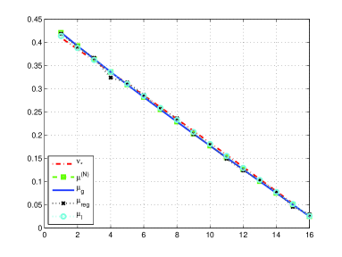
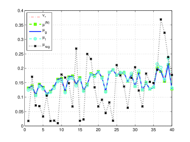
Figure 1: [left panel] Asian Option when $(\upsilon,K,\nu)=(0.1,45,\nu_{\star})$: drift vector $\nu_{\star}$ and directions $\mu^{(N)}$, $\mu_{\mathsf{g}}$, $\mu_{\mathrm{reg}}$ and $\mu_{l}$. $\nu_{\star}$ has been scaled to have norm $1$ ($\nu_{\star}\leftarrow\nu_{\star}/0.42$). [right panel] Basket Option when $(c,K,\nu)=(0.1,45,\nu_{\star})$: drift vector $\nu_{\star}$ and directions $\mu^{(N)}$, $\mu_{\mathsf{g}}$, $\mu_{l}$, $\mu_{\mathrm{reg}}$ and $\mu_{l}$. $\nu_{\star}$ has been scaled to have norm $1$ ($\nu_{\star}\leftarrow\nu_{\star}/0.41$).

In Figure 2, the successive directions $t\mapsto\mu^{(t)}$, the successive estimations of the quantity of interest $t\mapsto\mathcal{E}^{(t)}$ and of the variance $t\mapsto(\sum_{\mathbf{i}}p_{\mathbf{i}}\hat{\sigma}_{\mathbf{i}}^{(t)})^{2}$ are displayed. We observe that $\{\mu^{(t)},t\geq 0\}$ converges to the direction $\mu_{\mathsf{g}}$, and the convergence takes place after about 30 iterations. We find the same pattern for a wide range of parameter values. The choice of the stratification direction has a major impact on the variance of the estimate $\mathcal{E}^{(t)}$ as shown on Figure 2 [bottom right]. Along the iterations of the algorithm, the variance decreases from $0.1862$ to $0.0016$. We also observed that the convergence of the algorithm and the limiting values were independent of the initial values $(\mu^{(0)},M^{(0)})$ (these results are not reported for brevity). These initial values (and the choice of the sequence $\{\gamma^{(t)},t\geq 1\}$) only influence the number of iterations required to converge.

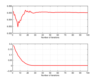
Figure 2: Asian Option when $(\upsilon,K,\nu)=(0.1,45,\nu_{\star})$. [left panel] successive directions of stratification $t\mapsto\mu^{(t)}$. $\mu^{(0)}$ is proportional to the vector $(1,\cdots,1)$ so that the $d$ curves start from the same point $1/\sqrt{d}$. By convention, the first component of $\mu^{(t)}$ is positive. [top right] successive estimations of the quantity of interest $t\mapsto\mathcal{E}^{(t)}$. [bottom right] successive values of the variance $t\mapsto(\sum_{\mathbf{i}}p_{\mathbf{i}}\ \hat{\sigma}_{\mathbf{i}}^{(t)})^{2}$; the limiting value is $0.002$.

AdaptStr can also be seen as a procedure that computes a stratification direction and provides the associated optimal allocation. These quantities can then be used for running a (usual) stratification procedure with $M$ draws and for the optimal allocation. By doing such with $M=20\,000$, we obtain an estimate of the quantity $\operatorname{E}[\phi(Y)]$ equal to $6.05$ and of the variance equal to $0.002/M$. We can compare these results to the output of ${\tt GHS}$: this yields the same estimator of $\operatorname{E}[\phi(Y)]$ and a larger standard deviation equal to $0.014/M$. Observe that since $\mu^{(N)}=\mu_{\mathsf{g}}$, the two algorithms differ from the allocations in the strata.

We conclude this study of AdaptStr by illustrating the role of the drift vector $\nu$ (see Eq. 17). We report on Figure 3 the limiting direction $\mu^{(N)}$, the estimates $t\mapsto\mathcal{E}^{(t)}$ and the variance $t\mapsto(\sum_{\mathbf{i}}p_{\mathbf{i}}\hat{\sigma}_{\mathbf{i}}^{(t)})^{2}$ when $\nu=0$.

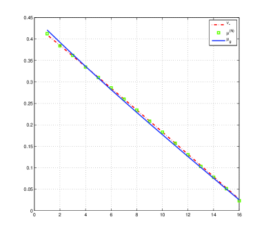
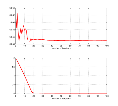
Figure 3: Asian Option with $(\upsilon,K,\nu)=(0.1,45,0)$: [left panel] the limiting direction $\mu^{(N)}$ and for comparison, $\mu_{g}$ and $\nu_{\star}$ normalised to have norm $1$ ($\nu_{\star}\to\nu_{\star}/0.42$). [top right] successive estimations of the quantity of interest $t\mapsto\mathcal{E}^{(t)}$. [bottom right] successive values of the variance $t\mapsto(\sum_{\mathbf{i}}p_{\mathbf{i}}\ \hat{\sigma}_{\mathbf{i}}^{(t)})^{2}$: the limiting value is $0.004$.

The limiting direction $\mu^{(N)}$ slightly differs from $\mu_{\mathsf{g}}$ and is close to $\nu_{\star}$. Moreover, the variance reduction is weaker: the limiting value of $t\mapsto(\sum_{\mathbf{i}}p_{\mathbf{i}}\hat{\sigma}_{\mathbf{i}}^{(t)})^{2}$ is $0.004$. The efficiency of the adaptive stratification procedure AdaptStr is thus related to the drift vector $\nu$ in (17); similar conclusions are reached in glasserman:heidelberger:shahabuddin:1999 (see also glasserman:2004 ).

We report in Tables 2 and 2 the variance of different estimators, as described in Section 5.2.

Insert Tables 2 and 2 about here

Consider first the case $\nu=0$. When the volatility of the asset is low $\upsilon=0.1$ and the strike is in-the-money, the performance of the adaptive stratification estimator ”AdaptStr” and of the stratification estimator with fixed direction $\mu_{\mathrm{reg}}$, $\mu_{\star}$ and $\mu_{l}$ and with optimal allocations are equivalent. We observe indeed that the directions $\mu^{(N)}$,$\mu_{\mathrm{reg}}$, $\mu_{\star}$ and $\mu_{l}$ are almost colinear. Compared to the plain Monte Carlo, the variance reduction factor is equal to 2500. The LH estimator with a rotation along any of the directions $\mu^{(N)}$,$\mu_{\star}$ and $\mu_{\mathrm{reg}}$ outperforms all the stratified estimators: the variance reduction is by a factor $10500$. This reduction in the variance strongly depends upon the choice of the rotation: the LH estimator with no rotation implies a variance reduction by a factor $150$.

When the volatility of the asset is high $\upsilon=1$, the conclusions are markedly different. Consider e.g. the case when the option is out of the money ($K=65$). The adaptive stratification estimator ”AdaptStr” provides a reduction of variance by a factor $150$, which is again similar to the variance reduction afforded by the stratification with fixed directions $\mu_{\mathrm{reg}}$, $\mu_{\star}$ and $\mu_{l}$, and optimal allocation; AdaptStr outperforms stratified estimators with any of the fixed direction $\mu_{\mathrm{reg}}$, $\mu_{\star}$ or $\mu_{l}$ by a factor $13$ when allocation is proportional. The LH estimator with no rotation only provides a reduction in variance by a factor $1.7$; when the rotation along $\mu^{(N)}$ is applied, the reduction is by a factor $65$. Here again, the LH estimator is very sensitive to the choice of the orthogonal matrix $O$.

The use of the drift $\nu=\nu^{\star}$ improves the variance of all the stratified estimators by a factor $2$ to $10$, depending on the choice of the stratification direction; and by a factor $10$ to $25$ for “MC”. Here again, ”AdaptStr” is the best stratified estimator; its performance can be approached by stratification estimators with fixed directions, but the choice of this fixed direction depends crucially upon the values of the volatility and the strike. The vectors $\mu^{(N)}$ and $\mu_{\mathrm{reg}}$ are almost colinear in many cases e.g. when $(\upsilon,K,\nu)=(0.1;45;\nu_{\star})$, but not always as observed in the case $(\upsilon,K,\nu)=(1;65;\nu_{\star})$ from the variances given in Table 2. It is interesting to note that the use of the drift $\nu_{\star}$ does not always improve the variance of the LH estimator.

These experiments show that the choice of the stratification direction and of the allocation is crucial. For example, in the case $(\upsilon,K,\nu)=(0.5,65,0)$, the adaptive stratification estimator improves upon the stratification estimator with fixed direction $(1,\cdots,1)/\sqrt{d}$ and optimal allocation by a factor $60$ (and by a factor $190$ when proportional allocation is used) - these results are not reported in the tables for brevity since this direction is rarely optimal - . Even if simple guesses for the direction reduce the variance, this reduction can be improved (by a factor $20$) when optimal allocation is used; this allocation is unknown and has to be learnt. In these examples, LH outperforms in many cases stratification procedures provided it is applied with a rotation $O$: the rotation along $\mu^{(N)}$ outperforms LH with no rotation and when compared with other simple guess rotations, it provides similar or better variance reduction. All these remarks strongly support the use of adaptive procedures.

5.4 Options with knock-out at expiration

A knock-out barrier option is a path-dependent option that expires worthless if the underlying reaches a specified barrier level. The payoff of this option is given by

$$\Xi(y)=\exp(-rT)\left(\frac{s_{0}}{d}\sum_{k=1}^{d}\exp\left((r-0.5\sigma^{2})\frac{kT}{d}+\sigma\sqrt{\frac{T}{d}}\sum_{j=1}^{k}y_{j}\right)-K\right)_{+}\mathbbm{1}_{\{S_{T}(y)\leq B\}}\;,$$

where $K$ is the strike price, $B$ is the barrier and $S_{T}(y)$ is the underlier price modeled as

$$S_{T}(y)=s_{0}\exp\left((r-0.5\sigma^{2})T+\sigma\sqrt{\frac{T}{d}}\sum_{j=1}^{d}y_{j}\right)\;.$$

In the numerical applications, we set $s_{0}=50$, $r=0.05$, $T=1$, $\sigma=0.1$, $d=16$ and $(K,B)\in\{(50,60),(50,80)\}$. We choose $\mu_{l}\propto(d,d-1,\cdots,1)$. On Figure 4[left panel], we plot $\mu^{(N)}$ in the case $(K,B,\nu)=(50,60,0)$; the limiting direction is $\mu_{l}$. On Figure 4[right panel], we plot $\mu^{(N)}$ in the case $(K,B,\nu)=(50,60,\nu_{\star})$; for comparison, we also plot $\nu_{\star}$, $\mu_{g}$, $\mu_{\mathrm{reg}}$ and $\mu_{l}$. This is an example where the optimal stratification direction $\mu^{(N)}$ does not coincide with the different directions of stratification ($\mu_{\mathsf{g}}$, $\mu_{\mathrm{reg}}$ and $\mu_{l}$); in this example, $\mu_{g}\sim\mu_{l}$ but the optimal direction of stratification is close to $(1,\cdots,1)/\sqrt{d}$. The direction associated to the regression estimator is far from being optimal.

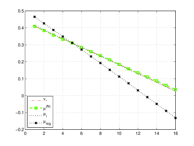
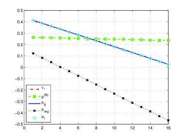
Figure 4: Barrier Option when $(K,B)=(50,60)$ and [left panel] $\nu=0$ or [right panel] $\nu=\nu_{\star}$: directions $\mu^{(N)}$, $\mu_{\mathrm{reg}}$, $\mu_{l}$, $\nu_{\star}$ and $\mu_{g}$. $\nu_{\star}$ has been scaled to have norm $1$ ($\nu_{\star}\leftarrow\nu_{\star}/0.84$)

We report in Tables 6 and 6 the variances of the different estimators, as described in Section 5.2.

Insert Table 6 and 6 about here

Consider first the case where the drift $\nu$ is set to $0$. When $(K,B)=(50,60)$ (the option is at the money, and the barrier is close to the money), the adaptive stratification provides a variance reduction by a factor 10 with respect to the plain Monte Carlo estimator. In this case, the stratification directions $\mu_{l}$ and $\mu_{\star}$ (with an optimal allocation) perform almost as well (and $\mu_{l}$ and $\mu_{\star}$ are close to $\mu^{(N)}$ at the convergence), while $\mu_{\mathrm{reg}}$ provides a higher variance. For the LH estimator, the variance reduction is only by a factor $1.5$. It is worthwhile to note that the best choices for the rotation , $\mu^{(N)}$ and $\mu_{\star}$, lead to a variance thrice the one of ”AdapStr”. The use of the drift vector $\nu_{\star}$ improves the variance of the adaptive stratification by a factor $1.8$; the optimal stratification vector is now $\mu^{(N)}$ which surpasses $\mu_{\mathrm{reg}}$. The variance of the LH estimator is also reduced.

When $(K,B)=(50,80)$ (the barrier is out of the money), a factor reduction 2800 is obtained by the adaptive stratification estimator ”AdaptStr”; a similar variance reduction is achieved using the stratified estimator with direction $\mu_{\mathrm{reg}}$ and with optimal allocation. For the LH estimator, the variance reduction is by a factor 2000, when the rotation is $\mu_{\mathrm{reg}}$. The use of the drift vector $\nu_{\star}$ improves the behavior of all the algorithms: the variance of “AdaptStr” is reduced by a factor $3.8$. Finally, LH with rotation $\mu^{(N)}$ reduces the variance of LH with no rotation by a factor $1200$.

To conclude, this example shows again the interest of adaptive procedures in order to find a stratification direction, the optimal allocation or a rotation in LH.

5.5 Basket options

Consider a portfolio consisting of $d$ assets. The portfolio contains a proportion $\alpha_{k}$ of asset $k$, $k\in\{1,\dots,d\}$. The price of each asset is described by a geometric Brownian motion (under the risk neutral probability measure)

$$\frac{dS_{t}^{(k)}}{S_{t}^{(k)}}=r\,dt+\upsilon_{k}\,dW_{t}^{(k)}$$

but the standard Brownian motions $\{W^{(k)}_{.},k\in\{1,\dots,d\}\}$ are not necessarily independent. For any $t\geq s$ and $k\in\{1,\dots,d\}$

$$\ln S^{(k)}_{t}=\ln S^{(k)}_{s}+\left(r-0.5\upsilon^{2}_{k}\right)(t-s)+\upsilon_{k}\sqrt{t-s}\tilde{Y}_{k}$$

where $\tilde{Y}=(\tilde{Y}_{1},\dots,\tilde{Y}_{d})\sim\mathcal{N}_{d}(0,\Sigma)$. The $d\times d$ matrix $\Sigma$ is a positive semidefinite matrix with diagonal coefficients equal to $1$. Therefore, the variance of the log-return on asset $k$ in the time interval $[s,t]$ is $(t-s)\upsilon^{2}_{k}$, and the covariance between the log-returns $i,j$ is $(t-s)\upsilon_{i}\upsilon_{j}\Sigma_{i,j}$. It follows that $\Sigma_{i,j}$ is the correlation between the log-returns. The price at time $0$ of a European call option with strike price $K$ and exercise time $T$ is given by $\operatorname{E}[\Xi(Y)]$ where

$$\Xi(y)=\exp(-rT)\left(\sum_{k=1}^{d}\alpha_{k}s_{0}^{(k)}\exp\left((r-0.5\upsilon^{2}_{k})T+\upsilon_{k}\sqrt{T}\tilde{y}_{k}\right)-K\right)_{+}$$

and $\tilde{y}=\sqrt{\Sigma}y$ ($\sqrt{\Sigma}$ denotes a square root of the matrix $\Sigma$ i.e. solves $MM^{T}=\Sigma$). In the numerical applications, $\Sigma$ is chosen to be $\Sigma_{i,j}=1_{\{i=j\}}+c1_{\{i\neq j\}}$, $\alpha_{k}=1/d$, $r=0.05$, $T=1$, and $d=40$. We consider $(c,K)\in\{(0.1,45),(0.5,45),(0.9,45)\}$. The initial values $\{s_{0}^{k},k\leq d\}$ are drawn from the uniform distribution in the range $[20,80]$; the volatilities $\{\upsilon_{k},k\leq d\}$ are chosen linearly equally spaced in the set $[0.1,0.4]$. The assets are sorted so that $\upsilon_{1}\leq\cdots\leq\upsilon_{d}$. We choose

$$\mu_{l}\propto\left(\alpha_{1}s_{0}^{(1)}\exp((r-0.5\upsilon^{2}_{1})T)\upsilon_{1},\cdots,\alpha_{d}s_{0}^{(d)}\exp((r-0.5\upsilon^{2}_{d})T)\upsilon_{d}\right)\sqrt{\Sigma}\;.$$

In the case $(c,K,\nu)=(0.1,45,\nu_{\star})$, we plot on Figure 1[right panel] the limiting direction $\mu^{(N)}$ and for comparison, the directions $\nu_{\star}$, $\mu_{g}$, $\mu_{\mathrm{reg}}$, $\mu_{l}$. We report in Tables 6 and 6 the variance of the different estimators, as described in Section 5.2.

Insert Tables 6 and 6 about here

In this example again the adaptive stratification estimator improves upon the best stratified estimator with (non-adaptive) stratification direction and optimal allocation. Here again, the optimal allocation improves the variance reduction, by a factor $15$ for example in the case $(c,K,\nu)=(0.9,45,0)$ for the fixed directions $\mu_{\mathrm{reg}}$, $\mu_{\star}$ or $\mu_{l}$. It is interesting to note that the variance reduction with respect to the plain Monte Carlo using ”AdaptStr” ranges from 100 ($c=0.1$,$K=45$) to 2500 ($c=0.9$,$K=45$) whereas the use of the drift $\nu^{\star}$ allows only a reduction by a factor 10. The choice of the stratification direction plays a more important role than the choice of drift direction.

The comparison with the LH estimator is more difficult, because this estimator behaves totally differently from the stratified estimator. First, except for $c=0.9$, the use of the drift $\nu_{\star}$ increases the variance: whereas the effect of the drift is always markedly beneficial for the Monte Carlo estimators, the drift $\nu_{\star}$ may increase the variance by a factor as large as 15 (when $(c,K)=(0.1,45)$). Second, LH with rotation always outperforms (adaptive) stratification: the main difficulty stems from the choice of the rotation but the obtained results show that rotation along $\mu^{(N)}$ provides either the maximal variance reduction or variance reduction similar to the best rotation among the three considered. Finally, the performance of the estimator is extremely sensitive to the choice of the simulation setting: when the correlation among the assets is large $c=0.9$, the choice of the first vector of the orthogonal matrix $O$ becomes crucial. With drift $\nu_{\star}$, rotation along $\mu^{(N)}$ (resp. $\mu_{\mathrm{reg}}$) improves LH with no rotation by a factor $22500$ (resp. $3000$).

5.6 Heston model of stochastic volatility

We consider a last example which is not covered by the methodology presented in glasserman:heidelberger:shahabuddin:1999 . We price an Asian option in the Heston model, specified as follows

$$d\xi_{t}=k(\theta-\xi_{t})dt+\sigma\sqrt{\xi_{t}}\,dW^{1}_{t},\;\;dS_{t}=rS_{t}dt+\sqrt{\xi_{t}}\,S_{t}\,(\rho dW^{1}_{t}+\sqrt{1-\rho^{2}}dW^{2}_{t}),\;\;dX_{t}=S_{t}dt$$

where $\{W^{1}_{t},t\geq 0\}$ and $\{W^{2}_{t},t\geq 0\}$ are two independent Brownian motions, $r$ is the risk free rate, $\sigma>0$ the volatility of the volatility process $\xi$, $k\geq 0$ the mean reversion rate, $\theta\geq 0$ the long run average volatility, and $\rho\in[-1,1]$ the correlation rate. The price of an Asian Call option with strike $K$ and maturity $T$ is

$$\operatorname{E}\left[\exp(-rT)\left(\frac{1}{T}X_{T}-K\right)_{+}\right].$$ (19)

In our tests, we have chosen the parameters so that $\sigma^{2}\leq 4k\theta$. This enabled us to replace by Gaussian increments the finitely-valued random variables used to discretize $W^{1}$ in the scheme proposed in alfonsi:2008 to approximate the SDE satisfied by $(S_{t},X_{t},\xi_{t})$. We refer to alfonsi:2008 for a precise description of the scheme that we used. The resulting approximation $\hat{X}_{d}$ of $X_{T}$ is generated from a vector $Y=(Y_{1},\ldots,Y_{d},Y_{d+1},\ldots,Y_{2d})\sim\mathcal{N}_{2d}(0,\mathrm{Id})$ corresponding to the increments of $(W^{1},W^{2})$ and a vector $B=(B_{1},\ldots,B_{d})$ of independent Bernoulli random variables with parameter $0.5$. The price (19) is then approximated by

$$\operatorname{E}[\exp(-rT)\left(\hat{X}_{d}-K\right)_{+}].$$

In the following tests we keep $\nu$ in (17) equal to zero and do not stratify the random vector $B$.

We choose $S_{0}=100$, $\theta=0.01$, $k=2$, $\sigma=0.2$, $T=1$, $r=0.095$, $\rho=-0.5$ and $(\xi_{0},K)\in\{(0.01,120),(0.01,100),(0.01,80),(0.04,130),(0.04,100),(0.04,70)\}$. The discretization step of the scheme is $d=50$.

On Figure 5 we plot the successive estimations of the variance $t\mapsto(\sum_{\mathbf{i}}p_{\mathbf{i}}\hat{\sigma}_{\mathbf{i}}^{(t)})^{2}$, when $(\xi_{0},K)=(0.01;120)$ and $(\xi_{0},K)=(0.04;70)$.

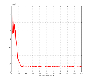
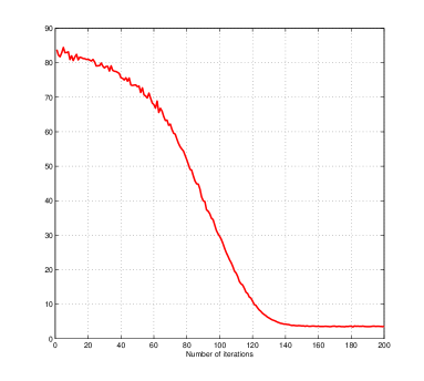
Figure 5: Asian Call Option in Heston model: successive estimations of the variance $t\mapsto(\sum_{\mathbf{i}}p_{\mathbf{i}}\ \hat{\sigma}_{\mathbf{i}}^{(t)})^{2}$ [left panel] when $(\xi_{0},K)=(0.01;120)$; [right panel] when $(\xi_{0},K)=(0.04;70)$

We plot on Figure 6 the components of $\mu^{(N)}$ with respect to the component index in the cases $(\xi_{0},K)=(0.01;120)$ and $(\xi_{0},K)=(0.04;70)$.

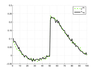
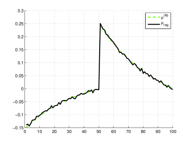
Figure 6: Asian Call Option in Heston model: vectors $\mu^{(N)}$ and $\mu_{\mathrm{reg}}$ in the cases [left panel] $(\xi_{0},K)=(0.01;120)$; [right panel] $(\xi_{0},K)=(0.04;70)$

We report in Tables 7 and 8 the variances of some estimators described in Section 5.2.

Insert Table 7 and 8 about here

The first observation is that even in this case, AdaptStr still works and provides variance reduction when compared to Monte Carlo. It is all the more efficient than the option is out of the money : when $(\xi_{0},K,\nu)=(0.01,120,0)$, the variance reduction is by a factor $85$; when $(\xi_{0},K,\nu)=(0.04,130,0)$, the variance reduction is by a factor $105$. AdaptStr and stratification with fixed direction $\mu_{\mathrm{reg}}$ are equivalent, provided the last one is applied with optimal allocation, just necessitating again iterative procedures.

We can wonder on the effect of the moneyness and the volatility of the model on the variance reduction. As shown in Table 7, in general the achieved variance reduction is larger when the option is out of the money (for $K=130$ and $\xi_{0}=0.04$ the variance is divided by nearly $105$ when using AdaptStr). We also observe that stratification procedures outperform LH samplers when the option is out of the money, but LH is equivalent to stratification when the option is in the money.

6 Proofs

6.1 Proofs of Section 3

In the sequel, we denote $\mathcal{I}_{m}\stackrel{{\scriptstyle\mathrm{def}}}{{=}}\{1,\dots,I\}^{m}$ and $p_{\mathbf{i}}\sigma_{\mathbf{i}}\stackrel{{\scriptstyle\mathrm{def}}}{{=}}\sqrt{\left(\int_{\mathsf{S}_{\mathbf{i}}}f_{\mu}\ d\lambda\right)\left(\int_{\mathsf{S}_{\mathbf{i}}}\zeta_{\mu}f_{\mu}\ d\lambda\right)-\left(\int_{\mathsf{S}_{\mathbf{i}}}\psi_{\mu}f_{\mu}\ d\lambda\right)^{2}}$ in place of $p_{\mathbf{i}}(\mu)\sigma_{\mathbf{i}}(\mu)$.

Lemma 1

Let $\{\mathsf{S}_{\mathbf{i}},\mathbf{i}\in\mathcal{I}_{m}\}$ be given by (8).

1. $\forall\epsilon>0,\;\forall M>\epsilon^{-1},\;\sup_{\mathcal{Q}:\inf_{\mathbf{i}\in\mathcal{I}_{m}}q_{\mathbf{i}}\geq\epsilon}\ \left|M\varsigma_{I,M}^{2}(\mu,g,\mathcal{Q})-\sum_{\mathbf{i}\in\mathcal{I}_{m}}\frac{p_{\mathbf{i}}^{2}\sigma_{\mathbf{i}}^{2}}{q_{\mathbf{i}}}\right|\leq\frac{1}{M\epsilon(\epsilon-M^{-1})}\ \mathrm{Var}[\phi(Y)].$

2. Assume that $\mathop{\mathrm{essinf}}_{g\cdot\lambda}\left(\chi/g\right)>0$ and $\mathop{\mathrm{esssup}}_{\chi\cdot\lambda}\left(f_{\mu}/\chi\right)<+\infty$. Let $\epsilon>0$. For any $(I,M)$ such that $MI^{-m}\mathop{\mathrm{essinf}}_{g\cdot\lambda}\left(\chi/g\right)\geq 1+\epsilon$

   $$\left|M\varsigma_{I,M}^{2}(\mu,g,\mathcal{Q}_{\chi})-\sum_{\mathbf{i}\in\mathcal{I}_{m}}\frac{p_{\mathbf{i}}^{2}\sigma_{\mathbf{i}}^{2}}{q_{\mathbf{i}}(\chi)}\right|\leq\frac{(1+\epsilon^{-1})\mathrm{Var}[\phi(Y)]}{\mathop{\mathrm{essinf}}_{g\cdot\lambda}\left(\chi/g\right)}\ \frac{I^{m}}{M}\ \left(\mathop{\mathrm{esssup}}_{\chi\cdot\lambda}\left(\frac{f_{\mu}}{\chi}\right)\wedge\frac{I^{m}}{\mathop{\mathrm{essinf}}_{g\cdot\lambda}\left(\chi/g\right)}\right).$$

3. For any positive integers $M,I$ and real $\epsilon>1$,

   $$\left|M\varsigma_{I,M}^{2}(\mu,g,\mathcal{Q}^{\star}(\mu))-\sum_{\mathbf{i}\in\mathcal{I}_{m}}\frac{p_{\mathbf{i}}^{2}\,\sigma_{\mathbf{i}}^{2}}{q^{\star}_{\mathbf{i}}(\mu)}\right|\leq\mathrm{Var}[\phi(Y)]\ \left((1+\epsilon)\frac{I^{m}}{M}+\frac{1}{\epsilon-1}\right)\;,$$

   where $\mathcal{Q}^{\star}(\mu)=\{q^{\star}_{\mathbf{i}}(\mu),\mathbf{i}\in\mathcal{I}_{m}\}$ is the optimal allocation defined by (7).

Proof

By definition of $M_{\mathbf{i}}$ (see Eq. 4), $M_{\mathbf{i}}=0$ when $q_{\mathbf{i}}=0$ and $M_{\mathbf{i}}\geq 1$ when $q_{\mathbf{i}}\geq M^{-1}$. One may have $M_{\mathbf{i}}=1$ when $q_{\mathbf{i}}\in(0,M^{-1})$ but then $MM_{\mathbf{i}}^{-1}\leq q_{\mathbf{i}}^{-1}$. Hence,

$$\left|M\;\varsigma^{2}_{I,M}(\mu,g,\mathcal{Q})-\sum_{\mathbf{i}\in\mathcal{I}_{m}:q_{\mathbf{i}}>0}\ \frac{p_{\mathbf{i}}^{2}\sigma_{\mathbf{i}}^{2}}{q_{\mathbf{i}}}\right|\\ \leq\sum_{\mathbf{i}\in\mathcal{I}_{m},q_{\mathbf{i}}\geq 1/M}\ \left|\frac{Mq_{\mathbf{i}}-M_{\mathbf{i}}}{M_{\mathbf{i}}}\right|\frac{p_{\mathbf{i}}^{2}\sigma_{\mathbf{i}}^{2}}{q_{\mathbf{i}}}+\sum_{\mathbf{i}\in\mathcal{I}_{m}:0<q_{\mathbf{i}}<1/M}\ \frac{p_{\mathbf{i}}^{2}\sigma_{\mathbf{i}}^{2}}{q_{\mathbf{i}}}$$ (20)

(i) When $\inf_{i\in\mathcal{I}_{m}}q_{\mathbf{i}}\geq\epsilon>M^{-1}$, the second term in the rhs is null and since by (4), $Mq_{\mathbf{i}}-1<M_{\mathbf{i}}<Mq_{\mathbf{i}}+1$,

$$\sum_{\mathbf{i}\in\mathcal{I}_{m},q_{\mathbf{i}}\geq 1/M}\ \left|\frac{Mq_{\mathbf{i}}-M_{\mathbf{i}}}{M_{\mathbf{i}}}\right|\frac{p_{\mathbf{i}}^{2}\sigma_{\mathbf{i}}^{2}}{q_{\mathbf{i}}}\leq M^{-1}\ \left(\sup_{\mathbf{i}\in\mathcal{I}_{m},q_{\mathbf{i}}\geq 1/M}p_{\mathbf{i}}q_{\mathbf{i}}^{-1}\right)\sum_{\mathbf{i}\in\mathcal{I}_{m},q_{\mathbf{i}}\geq 1/M}\ (q_{\mathbf{i}}-M^{-1})^{-1}\ p_{\mathbf{i}}\sigma_{\mathbf{i}}^{2},$$ (21)

which yields the desired result upon noting that $p_{\mathbf{i}}q_{\mathbf{i}}^{-1}\leq q_{\mathbf{i}}^{-1}\leq\epsilon^{-1}$ and $\sum_{\mathbf{i}}p_{\mathbf{i}}\sigma_{\mathbf{i}}^{2}\leq\mathrm{Var}[\phi(Y)]$.

(ii) Under the stated assumptions, $q_{\mathbf{i}}(\chi)=\int_{\mathsf{S}_{\mathbf{i}}}\chi d\lambda\geq\mathop{\mathrm{essinf}}_{g\cdot\lambda}\left(\chi/g\right)\ \ I^{-m}$. Hence $Mq_{\mathbf{i}}\geq 1+\epsilon$ which implies that the second term in the rhs of (20) is null. This also implies that $q_{\mathbf{i}}-M^{-1}\geq\left(1-\frac{1}{1+\epsilon}\right)\mathop{\mathrm{essinf}}_{g\cdot\lambda}\left(\chi/g\right)\ I^{-m}$. We conclude the proof by combining this bound with (21) and the following one :

$$\frac{p_{\mathbf{i}}}{q_{\mathbf{i}}(\chi)}=\frac{\int_{\mathsf{S}_{\mathbf{i}}}f_{\mu}\ d\lambda}{\int_{\mathsf{S}_{\mathbf{i}}}\chi\ d\lambda}\leq\mathop{\mathrm{esssup}}_{\chi\cdot\lambda}\left(f_{\mu}/\chi\right)\wedge\frac{1}{q_{\mathbf{i}}(\chi)}\leq\mathop{\mathrm{esssup}}_{\chi\cdot\lambda}\left(f_{\mu}/\chi\right)\wedge\frac{I^{m}}{\mathop{\mathrm{essinf}}_{g\cdot\lambda}\left(\chi/g\right)}\;.$$

(iii) Note that by convention, $p_{\mathbf{i}}^{2}\sigma_{\mathbf{i}}^{2}/q^{\star}_{\mathbf{i}}(\mu)=0$ when $q^{\star}_{\mathbf{i}}(\mu)=0$. By definition of the optimal allocation (see Eq. 7),

$$p_{\mathbf{i}}^{2}\sigma_{\mathbf{i}}^{2}/q^{\star}_{\mathbf{i}}(\mu)=q^{\star}_{\mathbf{i}}(\mu)\left(\sum_{\mathbf{j}}p_{\mathbf{j}}\sigma_{\mathbf{j}}\right)^{2}\leq q^{\star}_{\mathbf{i}}(\mu)\ \mathrm{Var}[\phi(Y)]\;.$$

The second term in the rhs of (20) is upper bounded by $I^{m}M^{-1}\ \mathrm{Var}[\phi(Y)]$. For the first term,

$$[\mathrm{Var}[\phi(Y)]]^{-1}\ \sum_{\mathbf{i}\in\mathcal{I}_{n},q^{\star}_{\mathbf{i}}(\mu)\geq 1/M}\ \left|\frac{Mq^{\star}_{\mathbf{i}}(\mu)-M_{\mathbf{i}}}{M_{\mathbf{i}}}\right|\frac{p_{\mathbf{i}}^{2}\sigma_{\mathbf{i}}^{2}}{q^{\star}_{\mathbf{i}}(\mu)}\\ \leq\sum_{\mathbf{i}\in\mathcal{I}_{m},1/M\leq q^{\star}_{\mathbf{i}}(\mu)\leq\epsilon/M}\ \left|\frac{Mq^{\star}_{\mathbf{i}}(\mu)-M_{\mathbf{i}}}{M_{\mathbf{i}}}\right|\ q^{\star}_{\mathbf{i}}(\mu)+\sum_{\mathbf{i}\in\mathcal{I}_{m},q^{\star}_{\mathbf{i}}(\mu)\geq\epsilon/M}\ \left|\frac{Mq^{\star}_{\mathbf{i}}(\mu)-M_{\mathbf{i}}}{M_{\mathbf{i}}}\right|\ q^{\star}_{\mathbf{i}}(\mu)\;.$$

For all $\mathbf{i}$ such that $q^{\star}_{\mathbf{i}}(\mu)\geq 1/M$, $M_{\mathbf{i}}^{-1}|Mq^{\star}_{\mathbf{i}}(\mu)-M_{\mathbf{i}}|\leq 1$ which implies that

$$\sum_{\mathbf{i}\in\mathcal{I}_{m},1/M\leq q^{\star}_{\mathbf{i}}(\mu)\leq\epsilon/M}\ \left|\frac{Mq^{\star}_{\mathbf{i}}(\mu)-M_{\mathbf{i}}}{M_{\mathbf{i}}}\right|q^{\star}_{\mathbf{i}}(\mu)\leq\frac{\epsilon I^{m}}{M}\;.$$

For all $\mathbf{i}$ such that $q^{\star}_{\mathbf{i}}(\mu)\geq\epsilon/M$, $M_{\mathbf{i}}^{-1}|Mq^{\star}_{\mathbf{i}}(\mu)-M_{\mathbf{i}}|\leq M_{\mathbf{i}}^{-1}\leq(Mq^{\star}_{\mathbf{i}}(\mu)-1)^{-1}\leq(\epsilon-1)^{-1}$ which implies that

$$\sum_{\mathbf{i}\in\mathcal{I}_{m},q^{\star}_{\mathbf{i}}(\mu)\geq\epsilon/M}\ \left|\frac{Mq^{\star}_{\mathbf{i}}(\mu)-M_{\mathbf{i}}}{M_{\mathbf{i}}}\right|q^{\star}_{\mathbf{i}}(\mu)\leq(\epsilon-1)^{-1}\;.$$

Proof

of Proposition 1 To prove the Proposition 1, we need the two following Lemmas. The first is a standard change of variables formula (see for example, (dudley:2004, , Theorem 4.1.11)). Define $G^{-1}(x_{1},\dots,x_{m})\stackrel{{\scriptstyle\mathrm{def}}}{{=}}(G_{1}^{-1}(x_{1}),\dots,G_{m}^{-1}(x_{m}))$ where $G_{k}$ is the c.d.f. associated to the density $g_{k}$ on $\mathbb{R}$.

Lemma 2

Let $h:\mathbb{R}^{m}\rightarrow\mathbb{R}$ be a measurable function. Assume that $h$ is nonnegative or is such that $\int_{\mathbb{R}^{m}}|h|1_{\{g>0\}}\ d\lambda<+\infty$. Then, for all $0\leq v_{k}\leq w_{k}\leq 1$, $k\in\{1,\dots,I\}$

$$\int_{\prod_{k=1}^{m}[G^{-1}_{k}(v_{k}),G^{-1}_{k}(w_{k})]}h1_{\{g>0\}}\ d\lambda=\int_{\prod_{k=1}^{m}[v_{k},w_{k}]}\frac{h}{g}\circ G^{-1}\ d\lambda\;.$$ (22)

The second technical Lemma is our key approximation result.

Lemma 3

Let $h,\gamma:\mathbb{R}^{m}\to\mathbb{R}$ be functions such that $\int_{\mathbb{R}^{m}}\left(h^{2}+\gamma^{2}\right)/g\ d\lambda<+\infty$. Define for $\mathbf{i}\in\mathcal{I}_{m}$,

$$R_{\mathbf{i}}[h,\gamma]\stackrel{{\scriptstyle\mathrm{def}}}{{=}}\int_{\mathsf{S}_{\mathbf{i}}}h\gamma/g\ d\lambda-I^{m}\left(\int_{\mathsf{S}_{\mathbf{i}}}h\ d\lambda\right)\left(\int_{\mathsf{S}_{\mathbf{i}}}\gamma\ d\lambda\right)\;.$$ (23)

Then $\lim_{I\rightarrow+\infty}\sum_{\mathbf{i}\in\mathcal{I}_{m}}|R_{\mathbf{i}}[h,\gamma]|=0$.

Proof

By polarization, it is enough to prove the result when $\gamma=h$ with $\int_{\mathbb{R}^{m}}h^{2}/g\ d\lambda<+\infty$. This integrability condition ensures that $\lambda$-a.e. , $g=0$ implies $h=0$ and by (22), one has

$$R_{\mathbf{i}}[h,h]=\int_{\prod_{k=1}^{m}[(i_{k}-1)/I,i_{k}/I]}\frac{h^{2}}{g^{2}}\circ G^{-1}\ d\lambda-I^{m}\ \left(\int_{\prod_{k=1}^{m}[(i_{k}-1)/I,i_{k}/I]}\frac{h}{g}\circ G^{-1}\ d\lambda\right)^{2}\;,$$

where the right-hand-side is non-negative by Cauchy-Schwarz inequality. Set $\tilde{h}(u)\stackrel{{\scriptstyle\mathrm{def}}}{{=}}\frac{h}{g}(G^{-1}(u))$ if $u\in(0,1)^{m}$ and $0$ otherwise. By (22) and the integrability assumption made on $h$, the function $\tilde{h}$ is square integrable on $\mathbb{R}^{m}$. Using the definition of $\tilde{h}$ for the first equality and symmetry for the second one, one has

$$\sum_{\mathbf{i}\in\mathcal{I}_{m}}R_{\mathbf{i}}[h,h]=I^{m}\ \sum_{\mathbf{i}\in\mathcal{I}_{m}}\int_{\mathcal{J}_{\mathbf{i}}^{2}}\tilde{h}(u)\{\tilde{h}(u)-\tilde{h}(v)\}dudv=\frac{I^{m}}{2}\sum_{\mathbf{i}\in\mathcal{I}_{m}}\int_{\mathcal{J}_{\mathbf{i}}^{2}}\{\tilde{h}(u)-\tilde{h}(v)\}^{2}\ dudv\\ =\frac{I^{m}}{2}\sum_{\mathbf{i}\in\mathcal{I}_{m}}\int_{\mathcal{J}_{\mathbf{i}}}\int_{\mathcal{J}_{\mathbf{i}}-u}\{\tilde{h}(u)-\tilde{h}(u+w)\}^{2}\ dwdu\leq\frac{1}{2}\int_{[0,1]^{m}}\int_{[-1,1]^{m}}(\tilde{h}(u)-\tilde{h}(u+z/I))^{2}\ dudz\;.$$

where we have set, for $\mathbf{i}\in\mathcal{I}_{m}$, $\mathcal{J}_{\mathbf{i}}=\prod_{k=1}^{m}[(i_{k}-1)/I,i_{k}/I]$. By continuity of the translations in $L^{2}(\mathbb{R}^{m},du)$ and Lebesgue’s Theorem, one obtains that the right-hand-side converges to $0$ as $I\to\infty$.

We now proceed to the proof of Proposition 1. Under A1, it holds that

$$q_{\mathbf{i}}(\chi)\geq\left(\mathop{\mathrm{essinf}}_{g\cdot\lambda}\left(\chi/g\right)\right)\ \int_{\mathsf{S}_{\mathbf{i}}}g\ d\lambda=I^{-m}\ \mathop{\mathrm{essinf}}_{g\cdot\lambda}\left(\chi/g\right)\;.$$ (24)

Hence, by Lemma 1(i), to prove the first assertion, it is enough to check that $\lim_{I\rightarrow+\infty}\sum_{\mathbf{i}\in\{1,\dots,I\}^{m}}\frac{p_{\mathbf{i}}^{2}\;\sigma_{\mathbf{i}}^{2}}{q_{\mathbf{i}}(\chi)}=\varsigma^{2}_{\infty}(\mu,\chi)$. By definition of $R_{\mathbf{i}}$ (see Eq. (23)),

$$\frac{p_{\mathbf{i}}^{2}\;\sigma_{\mathbf{i}}^{2}}{q_{\mathbf{i}}(\chi)} =\frac{\int_{\mathsf{S}_{\mathbf{i}}}f_{\mu}^{2}(\zeta_{\mu}-\psi_{\mu}^{2})/g\ d\lambda-R_{\mathbf{i}}[f_{\mu},\zeta_{\mu}f_{\mu}]+R_{\mathbf{i}}[\psi_{\mu}f_{\mu},\psi_{\mu}f_{\mu}]}{I^{m}\ \int_{\mathsf{S}_{\mathbf{i}}}\chi\ d\lambda}\;,$$

$$\varsigma^{2}_{\infty}(\mu,\chi) =\sum_{\mathbf{i}\in\mathcal{I}_{m}}\frac{\int_{\mathsf{S}_{\mathbf{i}}}f_{\mu}^{2}(\zeta_{\mu}-\psi_{\mu}^{2})/g\ d\lambda-R_{\mathbf{i}}[\chi,f_{\mu}^{2}(\zeta_{\mu}-\psi_{\mu}^{2})/\chi]}{I^{m}\ \int_{\mathsf{S}_{\mathbf{i}}}\chi\ d\lambda}.$$

$$\mbox{Therefore }\sum_{\mathbf{i}\in\mathcal{I}_{m}}\frac{p_{\mathbf{i}}^{2}\;\sigma_{\mathbf{i}}^{2}}{q_{\mathbf{i}}(\chi)}-\varsigma^{2}_{\infty}(\mu,\chi)=\sum_{\mathbf{i}\in\mathcal{I}_{m}}\frac{R_{\mathbf{i}}[\chi,f_{\mu}^{2}(\zeta_{\mu}-\psi_{\mu}^{2})/\chi]+R_{\mathbf{i}}[\psi_{\mu}f_{\mu},\psi_{\mu}f_{\mu}]-R_{\mathbf{i}}[f_{\mu},\zeta_{\mu}f_{\mu}]}{I^{m}\ \int_{\mathsf{S}_{\mathbf{i}}}\chi\ d\lambda},$$

and one easily concludes with (24) and Lemma 3 (which applies under A2 and A3). The second assertion is a consequence of Lemma 1(ii).

Proof

of Proposition 2 Since for $a,b\geq 0$, $|\sqrt{a}-\sqrt{b}|\leq\sqrt{|a-b|}$, one has

$$\sum_{\mathbf{i}\in\mathcal{I}_{m}}\bigg{|}p_{\mathbf{i}}\sigma_{\mathbf{i}} -\int_{\mathsf{S}_{\mathbf{i}}}\left[f_{\mu}\sqrt{\zeta_{\mu}-\psi_{\mu}^{2}}\right]\ d\lambda\bigg{|}$$

$$\leq\sum_{\mathbf{i}\in\mathcal{I}_{m}}\bigg{|}\int_{\mathsf{S}_{\mathbf{i}}}f_{\mu}\ d\lambda\int_{\mathsf{S}_{\mathbf{i}}}\zeta_{\mu}f_{\mu}\ d\lambda-\bigg{(}\int_{\mathsf{S}_{\mathbf{i}}}\psi_{\mu}f_{\mu}\ d\lambda\bigg{)}^{2}-\bigg{(}\int_{\mathsf{S}_{\mathbf{i}}}\left[f_{\mu}\sqrt{\zeta_{\mu}-\psi_{\mu}^{2}}\right]\ d\lambda\bigg{)}^{2}\bigg{|}^{1/2}$$

$$=\sum_{\mathbf{i}\in\mathcal{I}_{m}}\sqrt{\frac{1}{I^{m}}\left|-R_{\mathbf{i}}[f_{\mu},\zeta_{\mu}f_{\mu}]+R_{\mathbf{i}}[\psi_{\mu}f_{\mu},\psi_{\mu}f_{\mu}]+R_{\mathbf{i}}[f_{\mu}\sqrt{\zeta_{\mu}-\psi_{\mu}^{2}},f_{\mu}\sqrt{\zeta_{\mu}-\psi_{\mu}^{2}}]\right|}$$

$$\leq\left(\sum_{\mathbf{i}\in\mathcal{I}_{m}}\left|-R_{\mathbf{i}}[f_{\mu},\zeta_{\mu}f_{\mu}]+R_{\mathbf{i}}[\psi_{\mu}f_{\mu},\psi_{\mu}f_{\mu}]+R_{\mathbf{i}}[f_{\mu}\sqrt{\zeta_{\mu}-\psi_{\mu}^{2}},f_{\mu}\sqrt{\zeta_{\mu}-\psi_{\mu}^{2}}]\right|\right)^{1/2}\;.$$

Under A2, $\int f_{\mu}^{2}(\zeta_{\mu}-\psi_{\mu}^{2})/g\ d\lambda<+\infty$, and by Lemma 3, the right-hand-side converges to $0$ as $I\to+\infty$. Therefore,

$$\lim_{I\to+\infty}\sum_{\mathbf{i}\in\mathcal{I}_{m}}\bigg{|}p_{\mathbf{i}}\sigma_{\mathbf{i}}-\int_{\mathsf{S}_{\mathbf{i}}}\left[f_{\mu}\sqrt{\zeta_{\mu}-\psi_{\mu}^{2}}\right]\ d\lambda\bigg{|}=0\;.$$ (25)

We now write

$$\left(\int_{{\mathbb{R}}^{m}}\left[f_{\mu}\sqrt{\zeta_{\mu}-\psi_{\mu}^{2}}\right]\ d\lambda\right)\ \sum_{\mathbf{i}\in\mathcal{I}_{m}}\left|q_{\mathbf{i}}(\chi_{\mu}^{\star})-q^{\star}_{\mathbf{i}}(\mu)\right|\\ \leq\sum_{\mathbf{i}\in\mathcal{I}_{m}}q^{\star}_{\mathbf{i}}(\mu)\left|\sum_{\mathbf{j}\in\mathcal{I}_{m}}p_{\mathbf{j}}\sigma_{\mathbf{j}}-\int\left[f_{\mu}\sqrt{\zeta_{\mu}-\psi_{\mu}^{2}}\right]\ d\lambda\right|+\sum_{\mathbf{i}\in\mathcal{I}_{m}}\left|p_{\mathbf{i}}\sigma_{\mathbf{i}}-\int_{\mathsf{S}_{\mathbf{i}}}\left[f_{\mu}\sqrt{\zeta_{\mu}-\psi_{\mu}^{2}}\right]\ d\lambda\right|\;.$$

By Eq.(25), the rhs tends to zero as $I\to+\infty$. The second assertion is a consequence of Lemma 1(iii) applied with $\epsilon=\sqrt{M/I^{m}}$ and of Eq. (25).

6.2 Proofs of Section 4

We only give the proof of Proposition 3 and refer to etore:fort:jourdain:moulines:2008 for the one of Corollary 1.

Proof

of Proposition 3 Let $H\in\mathbb{R}^{d}$ be such that $|H|<|\mu|$, $e_{1}=\frac{\mu}{|\mu|}$, $a=\left\langle H,e_{1}\right\rangle$, $b=|H-ae_{1}|$ and $e_{2}$ be equal to $\frac{H-ae_{1}}{b}$ if $b\neq 0$ and to any vector with norm $1$ orthogonal to $e_{1}$ otherwise. We complete $(e_{1},e_{2})$ with $(e_{3},\ldots,e_{d})$ to obtain an orthonormal basis of ${\mathbb{R}}^{d}$. For $\alpha\in{\mathbb{R}}^{d}$, $\alpha_{k}=\left\langle\alpha,e_{k}\right\rangle$.

$$g_{z}(\mu+H)-g_{z}(\mu) =\int_{\{\alpha,\alpha_{1}\leq\frac{z-\alpha_{2}b}{|\mu|+a}\}}h(\alpha)\;d\alpha-\int_{\{\alpha,\alpha_{1}\leq\frac{z}{|\mu|}\}}h(\alpha)\;d\alpha=\int_{{\mathbb{R}}^{d-1}}\int_{\frac{z}{|\mu|}}^{\frac{z-\alpha_{2}b}{|\mu|+a}}h(\alpha)d\alpha_{1}d\alpha_{2:d}$$

$$=-\int_{{\mathbb{R}}^{d-1}}\int_{0}^{1}h\left(\frac{z-\alpha_{2}bs}{|\mu|+as}e_{1}+\sum_{k=2}^{d}\alpha_{k}e_{k}\right)\frac{az+\alpha_{2}b|\mu|}{(|\mu|+as)^{2}}dsd\alpha_{2:d}$$

$$=-\int_{0}^{1}\int_{{\mathbb{R}}^{d-1}}h\left(z\frac{(|\mu|+as)e_{1}+bse_{2}}{(|\mu|+as)^{2}+(bs)^{2}}+\sum_{k=3}^{d}\alpha_{k}e_{k}\phantom{+\left(\alpha_{2}-\frac{zbs}{(|\mu|+as)^{2}+(bs)^{2}}\right)\frac{(|\mu|+as)e_{2}-bse_{1}}{|\mu|+as}}\right.$$

$$\left.\phantom{\sum_{k=3}^{d}\alpha_{k}e_{k}}+\left(\alpha_{2}-\frac{zbs}{(|\mu|+as)^{2}+(bs)^{2}}\right)\frac{(|\mu|+as)e_{2}-bse_{1}}{|\mu|+as}\right)\frac{az+\alpha_{2}b|\mu|}{(|\mu|+as)^{2}}d\alpha_{2:d}ds$$

$$=-\int_{0}^{1}\int h(y)\frac{\left\langle y,H\right\rangle}{|\mu+sH|}d\lambda^{\mu+sH}_{z}ds\;,$$ (26)

where, for the last equality, we made the change of variable

$$\beta_{2}=\frac{\sqrt{(|\mu|+as)^{2}+(bs)^{2}}}{|\mu|+as}\alpha_{2}-\frac{zbs}{(|\mu|+as)\sqrt{(|\mu|+as)^{2}+(bs)^{2}}}\;,$$

used the equality $(|\mu|+as)e_{1}+bse_{2}=\mu+sH$ and remarked that $\left\langle\mu+sH,y\right\rangle=z$ implies that $az+\left\langle y,e_{2}\right\rangle b|\mu|=(|\mu|+as)\left\langle y,H\right\rangle$. Define, for $\nu\in{\mathbb{R}}^{d}_{*}$, $\gamma(h,\nu)\stackrel{{\scriptstyle\mathrm{def}}}{{=}}\int\frac{y}{|\nu|}h(y)d\lambda^{\nu}_{z}$. We deduce that

$$g_{z}(\mu+H)-g_{z}(\mu)+\left\langle H,\int\frac{y}{|\mu|}\;h\bigl{(}y\bigr{)}\;d\lambda_{z}^{\mu}\right\rangle=\left\langle H,\int_{0}^{1}\{\gamma(h,\mu)-\gamma(h,\mu+sH)\}\,ds\right\rangle\;.$$

Consider now the following decomposition $\gamma(h,\nu)=\gamma\left(h\mathbbm{1}_{\{|\cdot|>M\}},\nu\right)+\gamma\left(h\mathbbm{1}_{\{|\cdot|\leq M\}},\nu\right)$. Under assumption (15), the first term in the rhs is arbitrarily small as $M$ goes to infinity uniformly in $\nu$ close to $\mu$. When $\nu\to\mu$, the measure $\mathbbm{1}_{\{|\cdot|\leq M\}}\lambda_{z}^{\nu}$ converges weakly to $\mathbbm{1}_{\{|\cdot|\leq M\}}\lambda_{z}^{\mu}$; hence, the second term converges to $\gamma\left(h\mathbbm{1}_{\{|\cdot|\leq M\}},\mu\right)$. Therefore, the function $\nu\mapsto\gamma(h,\nu)$ is continuous at $\mu$ and the conclusion follows easily.

Model				Price	Variance
$\upsilon$	$K$	$\nu$	$q_{i}$	-	MC	AdaptStr	GHS	$\mu_{\mathrm{reg}}$	$\mu_{\star}$	$\mu_{l}$
0.1	45	0	prop	6.05	8.640	-	-	0.017	0.016	0.017
			opt	6.05	8.640	0.004	-	0.005	0.004	0.004
		$\nu_{\star}$	prop	6.05	0.803	-	0.014	0.014	0.008	0.007
			opt	6.05	0.803	0.002	-	0.005	0.002	0.002
0.5	45	0	prop	9.00	158.1	-	-	2.086	2.128	2.243
			opt	9.00	158.1	0.352	-	0.362	0.371	0.390
		$\nu_{\star}$	prop	9.00	14.95	-	0.203	0.225	0.324	0.221
			opt	9.00	14.95	0.147	-	0.162	0.223	0.162
0.5	65	0	prop	2.16	48.41	-	-	1.857	1.859	2.097
			opt	2.16	48.41	0.093	-	0.096	0.096	0.147
		$\nu_{\star}$	prop	2.16	2.32	-	0.039	0.046	0.048	0.049
			opt	2.16	2.32	0.020	-	0.024	0.025	0.026
1	45	0	prop	14.01	852.0	-	-	52.24	54.51	57.72
			opt	14.01	852.0	5.39	-	5.48	5.69	6.02
		$\nu_{\star}$	prop	14.01	42.76	-	3.014	3.185	4.360	3.265
			opt	14.01	42.76	2.270	-	2.400	3.220	2.450
1	65	0	prop	7.79	587	-	-	50.9	50.5	55.8 ;
			opt	7.79	587	3.75	-	3.01	3.08	3.95
		$\nu_{\star}$	prop	7.78	22.34	-	1.55	1.75	2.01	1.56
			opt	7.78	22.34	0.99	-	1.14	1.31	1.00

Table 1: Asian Option: Monte Carlo and stratification

Model			Price	Variance
$\upsilon$	$K$	$\nu$		Latin	Latin +Rot $\mu_{\mathrm{reg}}$	Latin +Rot $\mu_{\star}$	Latin +Rot $\mu^{(N)}$
0.1	45	0	6.05	0.0596	0.0008)	0.0008	0.0008
		$\nu_{\star}$	6.05	0.6000	0.0063	0.0009	0.0003
0.5	45	0	9.00	35.55	0.374	0.351	0.385
		$\nu_{\star}$	9.00	11.72	0.166	0.242	0.137
0.5	65	0	2.16	27.55	0.152	0.135	0.147
		$\nu_{\star}$	2.16	2.00	0.043	0.037	0.033
1	45	0	14.00	357.70	10.86	9.84	12.20
		$\nu_{\star}$	14.00	36.25	2.35	3.25	2.10
1	65	0	7.78	339.11	7.94	7.70	9.14
		$\nu_{\star}$	7.78	19.62	1.49	1.34	1.25

Table 2: Asian Option: Latin Hypercube

Model				Price	Variance
$K$	$B$	$\nu$	$q_{i}$	-	MC	AdaptStr	GHS	$\mu_{\mathrm{reg}}$	$\mu_{\star}$	$\mu_{l}$
50	60	0	prop	1.38	2.99	-	-	1.46	1.13	1.14
			opt	1.38	2.99	0.31	-	0.83	0.31	0.31
		$\nu_{\star}$	prop	1.38	1.34	-	0.50	1.15	0.49	0.50
			opt	1.38	1.34	0.17	-	1.12	0.31	0.31
50	80	0	prop	1.92	4.92	-	-	0.016	0.017	0.016
			opt	1.92	4.92	0.002	-	0.002	0.002	0.002
		$\nu_{\star}$	prop	1.92	0.704	-	0.0011	0.0012	0.0013	0.0011
			opt	1.92	0.704	0.0005	-	0.0006	0.0006	0.0005

Table 3: Barrier Option: Monte Carlo and stratification

Model			Price	Variance
$K$	$B$	$\nu$		Latin	Latin +Rot $\mu_{\mathrm{reg}}$	Latin +Rot $\mu_{\star}$	Latin +Rot $\mu^{(N)}$
50	60	0	1.38	1.98	(1.5074; 1.5416)	0.97	0.98
		$\nu_{\star}$	1.38	1.26	1.01	0.31	0.21
50	80	0	1.92	0.727	0.002	0.002	0.002
		$\nu_{\star}$	1.92	0.4501	0.0005	0.0006	0.0004

Table 4: Barrier Option: Latin Hypercube

Model				Price	Variance
$c$	$K$	$\nu$	$q_{i}$	-	MC	AdaptStr	GHS	$\mu_{\mathrm{reg}}$	$\mu_{\star}$	$\mu_{l}$
0.1	45	0	prop	11.24	22.16	-	-	0.25	0.25	0.25
			opt	11.24	22.16	0.22	-	0.22;	0.22	0.22
		$\nu_{\star}$	prop	11.24	1.39	-	0.26	0.87	0.26	0.26
			opt	11.24	1.39	0.21	-	0.65	0.21	0.21
0.5	45	0	prop	11.56	51.13	-	-	0.37	0.37	0.37
			opt	11.56	81.13	0.10	-	0.10	0.10	0.10
		$\nu_{\star}$	prop	11.56	8.64	-	0.08	0.09	0.09	0.08
			opt	11.56	8.64	0.06	-	0.07	0.07	0.06
0.9	45	0	prop	12.09	134	-	-	0.75	0.74	0.74
			opt	12.09	134	0.05	-	0.05	0.05	0.05
		$\nu_{\star}$	prop	12.09	14.46	-	0.022	0.029	0.024	0.023
			opt	12.09	14.46	0.008	-	0.012	0.009	0.008

Table 5: Basket Option: Monte Carlo and stratification

Model			Price	Variance
$c$	$K$	$\nu$		Latin	Latin +Rot $\mu_{\mathrm{reg}}$	Latin +Rot $\mu_{\star}$	Latin +Rot $\mu^{(N)}$
0.1	45	0	11.24	0.08	0.07	0.03	0.03
		$\nu_{\star}$	11.24	1.18	0.92	0.05	0.04
0.5	45	0	11.56	4.94	0.02	0.02	0.02
		$\nu_{\star}$	11.56	6.90	0.02	0.02	0.02
0.9	45	0	12.09	13.05	0.007	0.006	0.007
		$\nu_{\star}$	12.09	12.51	0.0038	0.0026	0.0006

Table 6: Basket Option: Latin Hypercube

Model				Price	Variance
$\xi_{0}$	$K$	$\nu$	$q_{i}$	-	MC	AdaptStr	$\mu_{\mathrm{reg}}$
0.01	120	0	prop	0.007	0.0272	-	0.0234
			opt	0.007	0.0272	0.0003	0.0003
	100	0	prop	5.19	18.06	-	2.009
			opt	5.19	18.06	1.700	1.725
	80	0	prop	22.65	30.01	-	3.16
			opt	22.65	30.01	2.85	2.93
0.04	130	0	prop	0.024	0.152	-	0.098
			opt	0.024	0.152	0.001	0.001
	100	0	prop	6.42	46.58	-	2.37
			opt	6.42	46.58	1.69	1.68
	70	0	prop	31.74	88.38	-	4.08
			opt	31.74	88.38	3.58	3.71

Table 7: Asian Option in Heston model: Monte Carlo and stratification

Model			Price	Variance
$\xi_{0}$	$K$	$\nu$		Latin	Latin +Rot $\mu_{\mathrm{reg}}$	Latin +Rot $\mu^{(N)}$
0.01	120	0	0.007	0.027	0.008	0.009
	100	0	5.19	2.77	2.08	2.15
	80	0	22.65	3.65	2.37	2.20
0.04	130	0	0.024	0.15	0.03	0.03
	100	0	6.42	7.58	2.59	3.22
	70	0	31.74	3.19	3.81	3.54

Table 8: Asian Option in Heston model: Latin Hypercube

References

- (1) A. Alfonsi. High order discretization scheme for the CIR process: application to affine term structure and Heston model. Math. Comp., To appear (2009).
- (2) B. Arouna. Adaptative Monte Carlo method, a variance reduction technique. Monte Carlo Methods Appl., 10(1):1–24, 2004.
- (3) S. Asmussen and P. W. Glynn. Stochastic simulation: algorithms and analysis, volume 57 of Stochastic Modelling and Applied Probability. Springer, New York, 2007.
- (4) R. M. Dudley. Real analysis and probability, volume 74 of Cambridge Studies in Advanced Mathematics. Cambridge University Press, Cambridge, 2002. Revised reprint of the 1989 original.
- (5) P. Etore, G. Fort, B. Jourdain, and E. Moulines. On adaptive stratification. Technical report, ArXiv math.PR/0809.1135, 2008.
- (6) P. Etore and B. Jourdain. Adaptive optimal allocation in stratified sampling methods. Methodol. Comput. Appl. Probab., 9(2):117–152, to appear (2009).
- (7) P. Glasserman. Monte Carlo methods in financial engineering, volume 53 of Applications of Mathematics (New York). Springer-Verlag, New York, 2004. Stochastic Modelling and Applied Probability.
- (8) P. Glasserman, P. Heidelberger, and P. Shahabuddin. Asymptotically optimal importance sampling and stratification for pricing path-dependent options. Math. Finance, 9(2):117–152, 1999.
- (9) A. Judistsky, G. Lan, A. Nemirovski, and A. Shapiro. Stochastic approximation approach to stochastic programming. Technical report, 2007. http://www2.isye.gatech.edu/ nemirovs/.
- (10) R. Kawai. Adaptive Monte Carlo variance reduction with two-time-scale stochastic approximation. Monte Carlo Methods Appl., 13(3):197–217, 2007.
- (11) H. J. Kushner and G. Yin. Stochastic approximation and recursive algorithms and applications, volume 35 of Applications of Mathematics (New York). Springer-Verlag, New York, second edition, 2003. Stochastic Modelling and Applied Probability.
- (12) A. Owen. Quasi Monte Carlo sampling. In Monte Carlo Ray Tracing : Siggraph 2003 Course, 2003.
- (13) A. B. Owen. A central limit theorem for Latin hypercube sampling. J. Roy. Statist. Soc. Ser. B, 54(2):541–551, 1992.
- (14) G. Ch. Pflug. Optimization of stochastic models. The Kluwer International Series in Engineering and Computer Science, 373. Kluwer Academic Publishers, Boston, MA, 1996. The interface between simulation and optimization.
- (15) R. Y. Rubinstein and D. P. Kroese. The cross-entropy method. Information Science and Statistics. Springer-Verlag, New York, 2004. A unified approach to combinatorial optimization, Monte-Carlo simulation, and machine learning.
- (16) R. Y. Rubinstein and D. P. Kroese. Simulation and the Monte Carlo method. Wiley Series in Probability and Statistics. Wiley-Interscience [John Wiley & Sons], Hoboken, NJ, second edition, 2008.