The NLO corrections of $H_{TC}\Pi^{0}$and $\Pi^{+}\Pi^{-}$ pair production at the ILC in the TC2 model

Abstract

As well known, if the Higgs boson were not observed at LHC, the technicolor model would be the most favorable candidate responsible for the symmetry breaking. To overcome some defects in the previous model, some extended versions have been proposed. In the TC2 model typical signature is existence of heavy $H_{TC}$ and technipion $\Pi$. A direct proof of validity of the model is to produce them at accelerator. Thus we study the production rates of $e^{+}e^{-}\to H_{TC}\Pi^{0}$ and $e^{+}e^{-}\to\Pi^{+}\Pi^{-}$ at ILC in the topcolor-assisted technicolor (TC2) model. In fact, there is a flood of models belonging to new physics which can result in products with characteristics similar to $H_{TC}+\Pi$ of the TC2 model. Therefore to distinguish this model from others one may need to investigate some details by calculating the cross section to NLO. We indeed find that the NLO corrections are significant, namely the ratio $\delta\equiv(\sigma_{NLO}-\sigma_{LO})/\sigma_{LO}$ in $e^{+}e^{-}\to H_{TC}\Pi^{0}$ exceeds 100% within a plausible parameter space.

Keywords TC2, top-pion, top-higgs, LOOPTOOLS

1 Introduction

The success of the standard model (SM) is not doubtful at all. On the other aspect, however, the mechanism which breaks the electroweak symmetry is not yet quite understood. In the typical spontaneous symmetry breaking scheme the Higgs boson is required but it so far evaded observation. In addition, there exist the prominent problems of triviality and unnaturalness in the Higgs sector. Thus alternative dynamical symmetry breaking schemes were proposed, among the models, the technicolor model (TC) is the most favorable one which was proposed by Weinberg and Susskind [1, 2] independently.

The advantage of dynamical electroweak symmetry breaking (EWSB) is that there the elementary scalar field is not introduced to be responsible for the breaking, therefore, it can avoid the troubles of triviality and unnaturalness. However, the initial TC model is the simplest version and exposes some obvious defects. To remedy those defects, several modified version have appeared [3, 4] later. In order to explain the large mass difference between the top quark and the bottom quark, the topcolor-assisted technicolor (TC2) model was proposed by Hill [6, 7, 8] to improve the original one. Namely the TC2 model can naturally produce large top quark mass and realize dynamical electroweak symmetry breaking. Concretely, in this model, the top-color interaction makes a small contribution to the EWSB, but indeed is responsible for the main part of the top quark mass as $(1-\epsilon_{t})m_{t}$ where $\epsilon_{t}$ is a model-dependent parameter within a range of $0.03<\epsilon_{t}<0.1$ [9], whereas the TC interaction plays the main role for breaking the electroweak gauge symmetry. The extended TC (ETC) interaction gives rise to the masses of the ordinary fermions (quarks and leptons) and a small portion $\epsilon_{t}M_{t}$ of the top mass. One of the most general characteristics of the TC2 model is existence of three isospin-triplet pseudo-Goldstone bosons called as top-pions ( $\Pi^{\pm},\Pi^{0}$) and one isospin-singlet boson$-$the top-Higgs ($H_{TC}$). Obviously, such new particles do not exist in the SM, and their appearance can be treated as clear and definite signatures of the new physics beyond the SM. To be consistent with the SM phenomenology, the energy scale of the model must be sufficiently high, say at TeV order, so that one needs to look for direct production of such new particles at high energy experiments.

Definitely, the LHC would be the first place to carry out such exploration, but since at the hadron colliders, the background is very complicated and it is hard to identify the signal. Instead, in the ILC experiment which will be be running in the future, the situation is much better. Starting with a relatively simple situation, therefore in this work, we study a favorable channel for the electron-positron collisions and will carry out some rigorous calculation for the LHC case in our next work. Concretely, we consider the production process $e^{+}e^{-}\to H_{TC}\Pi^{0}$ and $e^{+}e^{-}\to\Pi^{+}\Pi^{-}$.

In our earlier work [5], the tree level contribution was considered and one noticed that such processes may be observable for the designed luminosity of ILC. On other aspect, there is a flood of new physics models which also result in similar production processes (with different new particles). To distinguish the TC2 model from others, some details about the production cross sections and differential cross sections are needed. At the tree level, some parameters are fed in by hand and only the order of magnitude is estimated as long as the NLO is significant, so that one cannot tell the difference of various models, thus the NLO calculation may become necessary. Therefore, in this paper, we carry out the calculation to NLO and we find that the NLO contribution is significant and moreover, NLO corrections are quite different for $e^{+}e^{-}\to H_{TC}\Pi^{0}$ and $e^{+}e^{-}->\to\Pi^{+}\Pi^{-}$.

This paper is organized as follows. In Section 2 we will present the theoretical formulation of the production rates for processes $e^{+}e^{-}\to H_{TC}\Pi^{0}$ and $e^{+}e^{-}\to\Pi^{+}\Pi^{-}$. By inputting the model parameters, we obtain the numerical resultsa in Section 3. Our conclusion and some discussions are drawn in the last section.

2 Theoretical Formulation

In this section, we will present the theoretical formulation of the cross sections for two processes $e^{+}e^{-}\to H_{TC}\Pi^{0}$ and $e^{+}e^{-}\to\Pi^{+}\Pi^{-}$ up to NLO in the TC2 model.

2.1 For $e^{+}e^{-}\to H_{TC}\Pi^{0}$

In the TC2 model there are three relatively light physical top-pions ( $\Pi^{\pm},\Pi^{0}$) whose couplings to $t$ and $b$ quarks are [10, 12, 13]:

$$\frac{m_{t}\tan\beta}{v}[iK_{UR}^{tt}K_{UL}^{tt*}\bar{t}_{L}t_{R}\Pi^{0}+\sqrt{2}K_{UR}^{tt}K_{DL}^{bb\ast}\bar{b}_{L}t_{R}\Pi^{-}+h.c.],$$ (1)

where $\tan\beta=\sqrt{(v/v_{\pi})^{2}-1}$ and the top-pion decay constant $v_{\pi}\simeq O(60-100)$ GeV[12, 13]. $v=\sqrt{2}v_{w}\approx 246$ GeV is the electro-weak symmetry breaking scale. $K_{UL}^{ij}$ are matrix elements of the unitary matrix $K_{UL}$ from which the Cabibbo-Kabayashi-Maskawa (CKM) matrix $V$ can be derived as $V=K_{UL}^{-1}K_{DL}$ and the matrices $K_{UL}$ and $K_{UL}$ are responsible for transforming the weak-engenstates into the mass-eigenstates of left-handed U-type and D-type quarks respectively. $K_{UR}^{ij}$ are the matrix elements of the corresponding right-handed rotation matrix $K_{UR}$. Their values can be found in Ref. [12, 13]:

$$K_{UL}^{tt}=K_{DL}^{bb}=1,\;\qquad K_{UR}^{tt}=1-\epsilon_{t}.$$ (2)

Here, there is a free parameter $0.03<\epsilon_{t}<0.1$ which was discussed in the relevant literature about how the heavy top quark and other light quarks obtain their masses from different sources [9].

The TC2 model also suggests existence of a scalar $H_{TC}$ called as the top-Higgs boson [10, 11], which is a $\overline{t}t$ bound state and analogous to the $\sigma$ boson which plays an important role for low energy phenomenology. Its couplings to quarks are in analog to that of the neutral top-pions. The Feynman rules related to the top-pions and the top-Higgs are shown below [11]:

$$\begin{array}[]{l}Z_{\mu}H_{TC}\Pi^{0}:\frac{\displaystyle g}{\displaystyle 2c_{w}}\frac{\displaystyle v_{T}}{\displaystyle v}(P_{\mu}^{H}-P_{\mu}^{0}),~{}~{}~{}~{}Z_{\mu}\Pi^{-}\Pi^{+}:i\frac{\displaystyle g}{\displaystyle c_{w}}(1-2s_{w}^{2})(P_{\mu}^{-}-P_{\mu}^{+}),\\ \\ A_{\mu}\Pi^{-}\Pi^{+}:ie(P_{\mu}^{-}-P_{\mu}^{+}),~{}~{}~{}~{}~{}~{}~{}~{}~{}~{}~{}~{}\bar{t}t\Pi^{0}:\frac{\displaystyle-m_{t}\tan\beta}{\displaystyle v}(1-\epsilon_{t})\gamma_{5},\\ \\ t\bar{b}\Pi^{+}:i\sqrt{2}\frac{\displaystyle m_{t}\tan\beta}{\displaystyle v}(1-\epsilon_{t})L,~{}~{}~{}~{}~{}~{}\bar{t}b\Pi^{-}:i\sqrt{2}\frac{\displaystyle m_{t}\tan\beta}{\displaystyle v}(1-\epsilon_{t})R,\\ \\ t\bar{t}H_{TC}:i\frac{\displaystyle m_{t}\tan\beta}{\displaystyle v}(1-\epsilon_{t}),\\ \\ \end{array}$$ (11)

where $v^{2}=v_{\pi}^{2}+v_{T}^{2}$ and $v_{T}$ is the techni-pion decay constant similar to that of regular pions, $L=(1-\gamma_{5})/2,~{}R=(1+\gamma_{5})/2,~{}s_{w}=sin\theta_{w}$ and $c_{w}=cos\theta_{w}$ ($\theta_{w}$ is the Weinberg angle).

With these interaction vertices, we can immediately write down the production amplitude of $e^{+}e^{-}\to H_{TC}\Pi^{0}$ at the tree level:

$$M^{0}=\frac{g^{2}}{2c_{w}^{2}}\frac{v_{T}}{v}\bar{v}(P_{1}^{{}^{\prime}})(\not{P_{2}}-\not{P}_{3})[-\frac{1}{4}(1-\gamma_{5})+s_{w}^{2}]u(P_{2}^{{}^{\prime}})\frac{1}{P_{1}^{2}-M_{Z}^{2}}$$ (12)

At the NLO level, The Feynman diagrams responsible for the process are shown in Fig. 2.1. When carrying out the loop integration, an ultraviolet (UV) divergences appears and one needs to renormalize the Z-t-t coupling to remove the UV divergence. In this work, we employ the modified renormalization scheme $\overline{MS}$.

The loop-induced amplitude is written as

$$M^{loop}=\frac{g^{2}}{2c_{w}^{2}}N\bar{v}(P_{1}^{{}^{\prime}})[f_{2}\not{{P_{2}}}+f_{3}\not{{P}}_{3}][-\frac{1}{4}(1-\gamma_{5})+s_{w}^{2}]u(P_{2}^{{}^{\prime}})\frac{1}{P_{1}^{2}-M_{z}^{2}},$$ (13)

where N is the regular color factor. Calculations of such loop diagrams are straightforward. Each loop integration is composed of some scalar loop functions [14], which are evaluated in terms of the code LOOPTOOLS [15, 16]. The explicit expressions of relevant form factors ($f_{2}$, $f_{3}$) are lengthy, so that we keep them in Appendix A. The NLO amplitude is then written as

$$M=M^{tree}+M^{loop}.$$ (14)

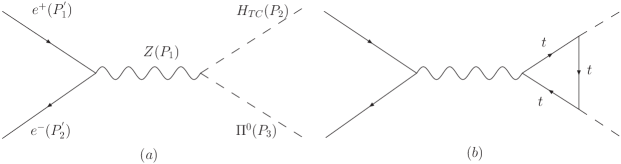
Figure 1: The Feynman diagrams for $e^{+}e^{-}\to H_{TC}\Pi^{0}$.

With the NLO amplitude, we have obtained the NLO differential cross section in the center-of-mass frame:

$$\frac{d\sigma_{NLO}}{d\Omega}=\frac{1}{2S}\frac{|\vec{P_{2}}|}{16\pi^{2}\sqrt{S}}\frac{1}{4}\sum\limits_{spins}{(|M^{0}|}^{2}+2Re[(M^{1})^{\dagger}M^{0}]+|M^{1}|^{2}).$$ (15)

Integration over the solid angle, we have the total cross section.

It is noticed that in the process $e^{+}e^{-}\to H_{TC}\Pi^{0}$, the ratio of $|M^{1}|^{2}/|M^{0}|^{2}\geq 0.20$ at most of the parameter spaces and cannot be thrown away.

2.2 For $e^{+}e^{-}\to\Pi^{+}\Pi^{-}$

The Feynman diagrams responsible for this process are shown in Fig. 2.2.

The tree level amplitude of $e^{+}e^{-}\to\Pi^{+}\Pi^{-}$ is:

$$\begin{array}[]{l}M^{0^{\prime}}=M_{\gamma}^{0^{\prime}}+M_{Z}^{0^{\prime}},\\ {}{}\\ M_{\gamma}^{0^{\prime}}=-i\frac{\displaystyle g^{2}s_{w}(1-2s_{w}^{2})}{\displaystyle c_{w}}\frac{\displaystyle 1}{\displaystyle P_{1}^{2}}\bar{v}(P_{1}^{{}^{\prime}})(\not{P}_{3}-\not{P}_{2})u(P_{2}^{{}^{\prime}}),\\ {}{}\\ M_{Z}^{0^{\prime}}=i\frac{\displaystyle g^{2}(1-2s_{w}^{2})}{\displaystyle c_{w}^{2}}\frac{\displaystyle 1}{\displaystyle P_{1}^{2}-M_{Z}^{2}}\bar{v}(P_{1}^{{}^{\prime}})(\not{P}_{3}-\not{P}_{2})[-\frac{\displaystyle 1}{\displaystyle 4}(1-\gamma_{5})+s_{w}^{2}]u(P_{2}^{{}^{\prime}}).\\ \end{array}$$ (21)

The loop-induced amplitude can be written in the form:

$$M^{loop^{\prime}}=M_{z}^{loop}+M_{\gamma}^{loop},$$ (22)

where the subscripts ”Z” and ”$\gamma$” correspond to the diagrams where $Z$ boson or photon is exchanged. By the Lorentz structure of the coupling, one can immediately show

$$M_{\gamma}^{loop}=0,$$

and then

$$M^{loop^{\prime}}=M_{z}^{loop}=\frac{\displaystyle g^{2}}{\displaystyle 2cw^{2}}N\bar{\displaystyle v}(P_{1}^{{}^{\prime}})[f_{2}^{{}^{\prime}}\not{P}_{2}+f_{3}^{{}^{\prime}}\not{P}_{3}][-\frac{\displaystyle 1}{\displaystyle 4}(1-\gamma_{5})+s_{w}^{2}]u(P_{2}^{{}^{\prime}})\frac{\displaystyle 1}{\displaystyle P_{1}^{2}-M_{z}^{2}}.\\$$ (23)

The explicit expressions of relevant form factors ($f_{2}^{{}^{\prime}}$, $f_{3}^{{}^{\prime}}$) are presented in Appendix A.

Figure 2: The Feynman diagrams for $e^{+}e^{-}\to\Pi^{+}\Pi^{-}$.

3 The numerical results

To obtain numerical results of the cross sections, we adopt the input parameters $M_{Z}=91.188$ GeV, $s_{w}^{2}=0.23$ and $v_{\pi}=100$ GeV. In our calculations the mass of top Higgs takes two different values: $M_{H}=200,\;300$ GeV [9]. The electromagnetic fine-structure constant $\alpha$ at the concerned energy scale is calculated by the renormalization group equation (RGE) with the boundary value $\alpha^{-1}=137.04$. Generally in the TC2 model, the mass of top pions is supposed to be around 200 GeV, for a phenomenological study, we let the mass vary within a narrow range of $150\sim 300$ GeV. Following the general discussion about the choice of center-of-mass energy for ILC, in our calculation it is set as $\sqrt{S}$ = 500 GeV [17]. The numerical results of the cross sections are shown in Fig. 3 and Fig. 3


Figure 3: Dependence of the cross section of $e^{+}e^{-}\to H_{TC}\Pi^{0}$ on top-pion mass $M_{\Pi}$ (150$\sim$300 GeV) for $M_{H}$ =200 GeV , $\epsilon_{t}=0.03$ (left) and $\epsilon_{t}=0.1$ (right) respectively.



Figure 4: Dependence of the cross section of $e^{+}e^{-}\to H_{TC}\Pi^{0}$ on top-pion mass $M_{\Pi}$ (150$\sim$200 GeV) for $M_{H}$ =300 GeV , $\epsilon_{t}=0.03$ (left) and $\epsilon_{t}=0.1$ (right) respectively.

The plots show that the cross section decreases with $M_{\Pi}$ and $M_{H_{TC}}$ and it is also noticed that as $\epsilon_{t}$ takes a value of 0.03 the cross section drops slightly faster than that for the case of $\epsilon_{t}=0.1$, namely it is not very sensitive to the value of $\epsilon$ which tells how the different sources contribute to the top quark mass. In general, the production rate is at the level of a few fb. Through the figures we also can observe that the loop-induced correction $\delta\equiv(\sigma_{NLO}-\sigma_{LO})/\sigma_{LO}$ exceeds 100% at most parameter spaces and even exceeds 130% for extreme situations. The dependence of $\delta$ on the input parameters can be seen in Table 1 of Appendix B.

The corresponding differential cross sections (DCS) are shown in Fig. 3 where the parameters are explicitly listed. From the figures, we can see that the DCS are symmetric with respect to $\pi/2$ and DCS decreases as $M_{\Pi}$ increases.

Figure 5: The dependence of the differential cross section of $e^{+}e^{-}\to\ H_{TC}\Pi^{0}$ on $\theta$.

If the ILC energy is upgraded up to 1 TeV [17] (i.e. $\sqrt{s}=1$ TeV), the NLO correction to the process will further increase as shown in Fig. 3:
Figure 6: The cross section of $e^{+}e^{-}\to H_{TC}\Pi^{0}$ with $\sqrt{s}=1$ TeV.

We can see that when $\sqrt{s}=1$ TeV, the NLO correction is even more important and $\delta$ exceeds that for $\sqrt{s}=500$ GeV.

The numerical results for $e^{+}e^{-}\to\Pi^{+}\Pi^{-}$ are shown in Fig. 3.

Figure 7: Dependence of The cross section of $e^{+}e^{-}\to\Pi^{+}\Pi^{-}$ on top-pion mass $M_{\Pi}$ (150$\sim$250 GeV) for $\epsilon_{t}=0.03$ (left) and $\epsilon_{t}=0.1$ (right) respectively.

The NLO corrections for $\sqrt{s}=1$ TeV are shown in Fig. 3:
Figure 8: Dependence of the differential cross section of $e^{+}e^{-}\to\Pi^{+}\Pi^{-}$ on $\theta$ with $\sqrt{s}=500$ GeV.


Figure 9: The cross section of $e^{+}e^{-}\to\Pi^{+}\Pi^{-}$ with $\sqrt{s}=1$ TeV.

The dependence of the relative correction $\delta$ on the input parameters is presented in the Table 2 of Appendix B.

Our results indicate that the NLO corrections to $e^{+}e^{-}\to\Pi^{+}\Pi^{-}$ are not as significant as to the $e^{+}e^{-}\to H_{TC}\Pi^{0}$, this is because there is an extra contribution from another tree diagram where a virtual photon serves as the intermediate state, thus the loop contributions are relatively smaller than the total tree contributions.

4 THE CONCLUSIONS AND OUTLOOK

Through the Tables in Appendix B, one can see that with yearly designed luminosity about 500 $fb^{-1}$ at ILC [17], if the detection efficiency can be 20%, more than several $10^{3}$ $H_{TC}\Pi^{0}$ and about $10^{4}$ $\Pi^{+}\Pi^{-}$ signals can be expected at ILC as long as the mass of relevant particles and corresponding parameters reside in a reasonable region, and if the luminosity can reach 1000 $fb^{-1}$, the amount of signals would be doubled and detection of such TC2 particles $\Pi^{\pm,0}$ and $H_{TC}$ would be very optimistic.

Our calculations indicate that the NLO contributions are important for the two concerned processes which may be crucial for detecting the TC2 model. The reason for larger NLO correction may be twofold. Firstly, in the loop, the intermediate states are top quark-antiquark whose mass in the TC2 theory is determined by two sources and expressed as [11]: $M_{t}=-\frac{\displaystyle 1}{\displaystyle\sqrt{2}}(Y_{t}f_{\pi}+\epsilon_{t}v_{T})$, and its TC Yukawa coupling $Y_{t}$ is high and causes an enhancement. Secondly, the extra color factor $N_{c}=3$ in the loop will further increase the loop-induced amplitude.

Because of the relative high one-loop contribution, one may naturally ask if two-loops contributions are necessary. If the two arguments listed above are the only reasons, we may expect that the two-loop contribution would not exceed the one-loop contribution.

The decay modes of $H_{TC}$, $\Pi^{\pm},\Pi^{0}$[21, 20] and a comparison with that in other models beyond the SM [18] at $e^{+}e^{-}$ linear colliders have been discussed in Ref. [5]. We do not intend to discuss these topics in this work, even though they are crucially important for observation, and will come back to it in our later work.

The advantage of analyzing such processes at the ILC is obvious that the hadronic background is very suppressed and the amount of signals may be practically observable. The calculation of the production at the $e^{+}e^{-}$ collision is relatively simple compared to the case for hadron colliders because there is no QCD correction and moreover, there does not exist the complicated infrared divergence which needs to be properly dealt with. By contrast, the situation would be deteriorated at the hadron colliders such as LHC, however, on other aspect, the production probability of the new physics particles at LHC may be much larger, so that the disadvantage caused by background contamination may be compensated. But definitely, one needs to consider the production rates of $H_{TC}$, $\Pi^{\pm},\Pi^{0}$ at LHC up to NLO and it would be our next work.

It is worth of noticing that, one may conjecture that a $H_{TC}$ pair or a $\Pi^{0}$ pair may also be produced at the one-loop level, but the results show that their contributions equal to zero due to an obvious symmetry constraints.

Our conclusion is that if the Higgs boson were not observed at LHC, the technicolor model would be favorable because it provides a dynamical symmetry breaking mechanism. Then one needs to look for evidence for existence or validity of the model, so detection of production of some specific particles which carry characteristics of the model would be a direct trace. We calculate the production rates of $e^{+}e^{-}\to\Pi^{+}\Pi^{-}$ and $e^{+}e^{-}\to H_{TC}\Pi^{0}$ at ILC to NLO, supposing its CM energy to be 500 GeV and find that the rates are sizable to be observed for a low background machine. In the calculations, we also notice that the NLO contributions for both modes are high compared to that of LO and then briefly analyze the reason. Therefore we indicate that to compare the theoretical prediction with data, one needs to carry out the calculation to NLO, moreover, our simple analysis may imply the NNLO should be smaller and less significant.

$\Large{\mathbf{APPENDIX}}$

Appendix A The explicit expressions of the form factors

The explicit expressions of the form factors $f_{i}$ used in the paper can be written as:

$$f_{2}=-\frac{1}{4\pi^{2}}[\frac{M_{t}\tan\beta}{v}(1-\epsilon_{t})]^{2}[B_{1}+(C_{1}+C_{11})(S+M_{\Pi}^{2}-M_{H}^{2})+(C_{2}+2C_{12})M_{\Pi}^{2}-C_{0}M_{t}^{2}+B_{0}],$$ (24)

$$\begin{array}[]{l}f_{3}=-\frac{\displaystyle 1}{\displaystyle 4\pi^{2}}[\frac{\displaystyle M_{t}\tan\beta}{\displaystyle v}(1-\epsilon_{t})]^{2}[B_{1}+C_{1}(M_{\Pi}^{2}-M_{H}^{2})+C_{11}(S+M_{\Pi}^{2}-M_{H}^{2})+(C_{2}+3C_{12})M_{\Pi}^{2}\\ {}{}{}{}{}{}\\ ~{}~{}~{}~{}~{}~{}-4C_{0}M_{t}^{2}+2C_{00}+2C_{22}M_{\Pi}^{2}+C_{12}(S-M_{H}^{2})].\\ \end{array}$$ (28)

$$C_{ij}=C_{ij}(P_{1}^{2},(-P_{2})^{2},(P_{1}-P_{2})^{2},M_{t}^{2},M_{t}^{2},M_{t}^{2}),$$ (29)

$$B_{0}=B_{0}((-P_{2})^{2},M_{t}^{2},M_{t}^{2}).$$ (30)

$$f_{2}^{{}^{\prime}}=i\frac{1}{4\pi^{2}}[\frac{M_{t}\tan\beta}{v}(1-\epsilon_{t})]^{2}[B_{0}^{{}^{\prime}}+B_{1}^{{}^{\prime}}+S(C_{1}^{{}^{\prime}}+C_{11}^{{}^{\prime}})+M_{\Pi}^{2}(C_{2}^{{}^{\prime}}+2C_{12}^{{}^{\prime}})+M_{t}^{2}C_{0}^{{}^{\prime}}],$$ (31)

$$\begin{array}[]{l}f_{3}^{{}^{\prime}}=i\frac{\displaystyle 1}{\displaystyle 4\pi^{2}}[\frac{\displaystyle M_{t}\tan\beta}{\displaystyle v}(1-\epsilon_{t})]^{2}[B_{1}^{{}^{\prime}}+S(C_{11}^{{}^{\prime}}+C_{12}^{{}^{\prime}})+M_{\Pi}^{2}(C_{2}^{{}^{\prime}}+2C_{12}^{{}^{\prime}}+2C_{22}^{{}^{\prime}}+M_{t}^{2}C_{0}^{{}^{\prime}}){}{}{}{}{}{}\\ {}\\ ~{}~{}~{}~{}~{}~{}+2C_{00}^{{}^{\prime}}-M_{t}^{2}C_{0}^{{}^{\prime}}].\\ \end{array}$$ (35)

$$C_{ij}^{{}^{\prime}}=C_{ij}^{{}^{\prime}}(P_{1}^{2},(-P_{2})^{2},(P_{1}-P_{2})^{2},M_{t}^{2},M_{t}^{2},M_{b}^{2}),$$ (36)

$$B_{0}^{{}^{\prime}}=B_{0}^{{}^{\prime}}((-P_{2})^{2},M_{t}^{2},M_{b}^{2}).$$ (37)

Here $B_{i}$, $C_{ij}$ are two-point and three-point scalar integrals. $P$ represents the momentum of relevant particle. The explicit Lorentz decompositions for the lowest order integrals take the forms given in Ref. [19]

Appendix B The ratio of $(\sigma_{NLO}-\sigma_{LO})/\sigma_{LO}$

Table 1: Dependence of $\delta$ on the parameter in $e^{+}e^{-}\to H_{TC}\Pi^{0}$

  $\epsilon_{t}$ $M_{H}$ $M_{\Pi}$ $\sigma_{NLO}$ $\sigma_{LO}$ $\delta$ 0.1 200 150 33.3611 15.9941 108.584% 175 26.7926 12.8525 108.462% 200 19.9713  9.6295 107.397% 225 13.4233  6.4926 106.749% 250  7.5164  3.6369 106.669% 275  2.4542  1.3117  87.098% 285  1.2881  0.6130 110.139% 295  0.2432  0.1184 105.321% 0.03 200 150 36.7804 15.9941 129.963% 175 29.5348 12.8525 129.798% 200 22.0070  9.6295 128.537% 225 14.7877  6.4926 127.764% 250  8.2565  3.6369 127.018% 275  2.6729  1.3117 103.772% 285  1.4235  0.6130 132.234% 295  0.2678  0.1184 126.100% 0.1 300 150  6.7968  3.2051 112.061% 160  5.0331  2.3744 111.975% 170  3.3789  1.5940 111.980% 180  1.8980  0.8953 111.989% 190  0.6914  0.3261 112.003% 195  0.2480  0.1170 112.012% 0.03 300 150  7.5093  3.2051 134.290% 160  5.5606  2.3744 134.191% 170  3.7331  1.5940 134.197% 180  2.0969  0.8953 134.209% 190  0.7639  0.3261 134.228% 195  0.2740  0.1170 134.240%  

Table 2: Dependence of $\delta$ on the parameter in $e^{+}e^{-}\to\Pi^{+}\Pi^{-}$

  $\epsilon$ $M_{\Pi}$ $\sigma_{NLO}$ $\sigma_{LO}$ $\delta$ 0.1 150 141.7408 107.4589 31.902% 160 127.8301  96.7722 32.093% 170 112.2826  84.3145 33.171% 180  95.9705  70.1459 36.815% 190  81.9590  60.6831 35.060% 200  63.6793  46.8669 35.872% 210  47.4190  34.9830 35.548% 220  32.1575  23.8273 34.960% 230  18.3033  13.7898 32.731% 240   7.1690   5.4693 31.076% 245   2.5796   1.9700 30.942% 0.03 150 148.3453 107.4589 38.048% 160 133.8350  96.7723 38.298% 170 117.7175  84.3145 39.617% 180 101.0672  70.1459 44.081% 190  86.1166  60.6831 41.911% 200  66.9610  46.8669 42.875% 210  49.8442  34.9830 42.481% 220  33.7806  23.8273 41.772% 230  19.1579  13.7898 38.928% 240   7.4997   5.4693 37.123% 245   2.6982   1.9700 36.962%

References

- [1] L. Susskind, Phys. Rev. D 20, 2619 (1979).
- [2] S. Weinberg, Phys. Rev. D 19, 1277 (1979).
- [3] S. Dimopoulos and L. Susskind, Nucl. Phys. B 155, 237 (1979).
- [4] E. Eichten and K. D. Lane, Phys. Lett. B 90, 125 (1980).
- [5] X. l. Wang, Q. p. Qiao and Q. l. Zhang, Phys. Rev. D 71, 095012 (2005).
- [6] C. T. Hill, Phys. Lett. B 345, 483 (1995) [arXiv:hep-ph/9411426].
- [7] K. D. Lane and E. Eichten, Phys. Lett. B 352, 382 (1995) [arXiv:hep-ph/9503433].
- [8] K. D. Lane, Phys. Lett. B 433, 96 (1998) [arXiv:hep-ph/9805254].
- [9] C. T. Hill and E. H. Simmons, Phys. Rept. 381, 235 (2003) [Erratum-ibid. 390, 553 (2004)] [arXiv:hep-ph/0203079].
- [10] G. Burdman, Phys. Rev. Lett. 83, 2888 (1999) [arXiv:hep-ph/9905347].
- [11] A. K. Leibovich and D. L. Rainwater, Phys. Rev. D 65, 055012 (2002) [arXiv:hep-ph/0110218].
- [12] H. J. He and C. P. Yuan, Phys. Rev. Lett. 83, 28 (1999) [arXiv:hep-ph/9810367].
- [13] H. J. He, S. Kanemura and C. P. Yuan, Phys. Rev. Lett. 89, 101803 (2002) [arXiv:hep-ph/0203090].
- [14] G. ’t Hooft and M. J. G. Veltman, Nucl. Phys. B 153, 365 (1979).
- [15] T. Hahn and M. Perez-Victoria, Comput. Phys. Commun. 118, 153 (1999) [arXiv:hep-ph/9807565].
- [16] T. Hahn, Nucl. Phys. Proc. Suppl. 135, 333 (2004) [arXiv:hep-ph/0406288].
- [17] James Brau, Yasuhiro Okada, Nicholas Walker [arXiv:0712.1950].
- [18] A. Djouadi, J. Kalinowski, P. Ohmann and P. M. Zerwas, Z. Phys. C 74, 93 (1997) [arXiv:hep-ph/9605339].
- [19] A. Denner, Fortsch. Phys. 41, 307 (1993) [arXiv:0709.1075 [hep-ph]].
- [20] C. x. Yue, Q. j. Xu, G. l. Liu and J. t. Li, Phys. Rev. D 63, 115002 (2001) [arXiv:hep-ph/0012332].
- [21] X. l. Wang, W. n. Xu, and L. l. Du, Commun. Theor. Phys. 41, 737(2004)
- [22] L. l. Chen, W. n. Xu, X. l. wang, HEP & NP 31, 232 (2007) (in Chinese)