Galactic Halos Derived from $\Lambda CDM$ Cosmology Simulation and their Red-Shift Evolution

Abstract

Galaxies can form in a sufficiently deep gravitational potential so that efficient gas cooling occurs. We estimate that such potential is provided by a halo of mass $M~{}_{\sim}^{>}~{}M_{c}\approx 7.0\times 10^{12}~{}(\Delta_{c}(z)(1+z)^{3})^{-1/2}~{}h^{-1}~{}M_{\odot}$, where $\Delta_{c}(z)$ is the mean overdensity of spherically virialized objects formed at redshift $z$, and $M_{c}\approx 4.0\times 10^{11}~{}h^{-1}~{}M_{\odot}$ at $z=0$. Based on this criterion, our galaxy samples are constructed from cosmology simulation data by using HiFOF to select subhalos in those FOF halos that are more massive than $M_{c}$. There are far more dark subhalos than galaxy-hosting subhalos. Several tests against observations have been performed to examine our galaxy samples, including the differential galaxy mass functions, the galaxy space density, the projected two point correlation functions (CF), the HODs, and the kinematic pair fractions. These tests show good agreements. Based on the consistency with observations, our galaxy sample is believed to correctly represent galaxies in real universe, and can be used to study other unexplored galaxy properties.

1 Introduction

The standard theoretical model for galaxy formation basically consists of two main elements, the cold dark matter (CDM) model and a dark energy field (which may take the form of a cosmological constant, $\Lambda$). The fundamental assumption made in the theory is that structure grew from weak density fluctuations present in the otherwise homogeneous and rapidly expanding early Universe. Afterwards, the gravitational instability drives these fluctuations into nonlinear regime in a bottom up fashion and they gradually grow to a wealth of structures today. Recent diverse cosmological studies, no matter from large-scale structure observations (e.g., Spergel et al., 2003), from supernova data (e.g., Riess et al., 1998), or from light element abundance (e.g., White et al., 1993), all seem to support the concordance model. Due to the highly nonlinear nature in the collapse of fluctuations and the subsequent hierarchical build-up of structure, numerical simulations come to play an indispensable role.

In the past thirty years, galaxy clustering has been intensively studied, as the clustering of galaxies has long been an essential testing ground for various cosmological models and galaxy formation scenarios. Especially due to the advent of modern computers, high resolution simulations become possible. Cosmological N-body simulations have developed into a powerful tool for calculating the gravitational clustering of collisionless dark matter from specified initial conditions. As the resolution of simulations increases, some numerical problems such as the overmerging problem (Klypin et al., 1999) can be overcome, and the galactic size scale in a large scale structure simulation can be resolvable. In addition, the growth of galaxy redshift surveys has led to measurements of increasing precision and detail. All these works have made the comparisons between theories and observations possible.

There are four main approaches used in cosmological simulations to study the galaxy clustering and properties. The first one is N-body plus hydrodynamical simulation including gas and dark matter particles (e.g., Weinberg et al., 2004). The second method is a hybrid method that combines N-body simulations of the dark matter component with semi-analytic treatments of the galaxy formation physics (e.g., Springel et al., 2005). Another approach is using high-resolution collisionless N-body simulations that identify galaxies with ”subhalos” in the dark matter distribution (e.g., Klypin et al., 1999; Kravtsov et al., 2004; Conroy et al., 2006). The last one is the so called Halo Occupation Distribution (HOD) approach which gives a purely statistical description of how dark matter halos are populated with galaxies (e.g., Berlind et al., 2003; Kravtsov et al., 2004; Zheng et al., 2005). It is known that the cold dark matter is the dominant mass component and it interacts only through gravity. To some extent, gravitational dynamics alone should explain the basic features of galaxy clustering. Neyrinck et al. (2004) tried to understand how the infrared-selected galaxies populate dark matter halos, paying special attention to the method of halo identification in simulations. They tested the hypothesis that baryonic physics negligibly affects the distribution of subhalos down to the smallest scales yet observed and successfully reproduced the Point Source Catalogue Redshift (PSCz) power spectrum. Berlind et al. (2003) reported that the HOD prediction of two methods, a semi-analytic model and gasdynamics simulations, agree remarkably well for samples of the same space density. This result indirectly supported the idea that the HOD, and hence galaxy clustering, is driven primarily by gravitational dynamics rather than by processes such as cooling and star formation. On the other hand, Kravtsov et al. (2004) adopt a variant of the bound density maxima (BDM) halo-finding algorithm (Klypin et al., 1999) to identify halos and subhalos and use the maximum circular velocity $V_{max}$ as a proxy of halo mass for selecting galaxy sample. Instead of selecting objects in a given range of $V_{max}$, at each epoch they selected objects of a set of number densities consistent with observational number densities and corresponding to (redshift dependent) thresholds in maximum circular velocity, i.e., $n_{i}(>V_{max})$. Their results show that the dependence of correlation amplitude on the galaxy number density in their sample is in general agreement with results from the Sloan Digital Sky Survey. Conroy et al. (2006) instead use the maximum circular velocity at the time of accretion, $V^{acc}_{max}$, for subhalos, and the results show agreement with the observed galaxy clustering in the SDSS data at $z\approx 0$ and in the DEEP2 samples at $z\approx 1$ over the range of separations, $0.1<r_{p}/(h^{-1}Mpc)<10.0$. However, this work lacks the information of the subhalo mass. Motivated by the results of these previous works, an approach similar to the galaxy identification with subhalos is adopted in this study. Despite some of our simulations include gas particles, we shall ignore the gas component in the identification of galaxies. Our approach in fact combines a subhalo finding algorithm, HiFOF, and a galaxy formation model. It ’directly’ locates where the galaxy should be formed and shows agreements with various observation results, such as galaxy mass function, two-point correlation function, etc. This result indicates that our galaxy identification model not only can successfully locate subhalos in simulations that reside inside host halos in real universe but also can give a galaxy mass function close to the observational one.

The paper is structured as follows. In section 2, we describe the simulation and the halo-finding algorithm in use. Thereafter, the galaxy halo model we adopt is discussed. In Section 3, we compare our galaxy samples with observations including the differential mass functions, the number density evolution, the correlation functions at different redshift, the halo occupation distribution, and the pair fraction. Finally, we discuss and summarize our results in Section 4.

2 Theoretical models

2.1 Simulations

Our simulations have been evolved in the concordance flat $\Lambda$CDM model: $\Omega_{0}=0.3,\Omega_{\Lambda}$ = 0.7, $\Omega_{b}=0.05$, and $h=0.66$, where $\Omega_{0}$, $\Omega_{\Lambda}$, $\Omega_{b}$ are the present-day matter, vacuum, and baryon densities and h is the dimensionless Hubble constant defined as $H_{0}$ $\equiv$ 100 $~{}h~{}km~{}s^{-1}~{}Mpc^{-1}$. These parameters are consistent with current observations on cosmological parameters (Spergel et al., 2003; Tegmark et al., 2004; Seljak et al., 2005; Sanchez et al., 2006) with $\Omega_{dm}$ = 0.20 $\pm$ 0.020, $\Omega_{b}$ = 0.042 $\pm$ 0.002, $\Omega_{\Lambda}$ = 0.76 $\pm$ 0.020, h = 0.74 $\pm$ 0.02. Four realizations with different box sizes and particle numbers were analyzed and compared to investigate the boundary and resolution effects as well as to have better statistics. GADGET1 (Springel et al., 2001b) and GADGET2 (Springel, 2005) were both employed to conduct the simulations. Our simulations all started at redshift $z=100$ and evolved to $z=0$, and their density spectra were normalized to $\sigma_{8}=0.94$, where $\sigma_{8}$ is the rms fluctuation in sphere of $8~{}h^{-1}~{}Mpc$ comoving radius. The first simulation ($\Lambda$$CDM_{100a}$) follows the evolution of $256^{3}$ dark matter particles and $256^{3}$ gas particles in a $100~{}h^{-1}~{}Mpc$ box on a side. The mass of a dark matter particle is $m_{dm}=$ 4.125 $\times 10^{9}~{}h^{-1}~{}M_{\odot}$, while the mass of a gas particle is $m_{gas}=$ 8.25 $\times 10^{8}$ $~{}h^{-1}~{}M_{\odot}$. In addition, We adopted a softening length switching from a comoving scale to a physical scale at $z=2.3$. The softening length $\epsilon$ was 20 $~{}h^{-1}~{}kpc$ (comoving) before redshift $z=2.3$. After that, $\epsilon$ was switched to $6~{}h^{-1}~{}kpc$ (physical). Thus, the highest force resolution is $6~{}h^{-1}~{}kpc$. The second simulation ($\Lambda$$CDM_{200}$) follows the evolution of $512^{3}$ dark matter particles and $512^{3}$ gas particles in the same cosmology but in a $200~{}h^{-1}~{}Mpc$ box on a side. Both dark matter particles and gas particles have the same masses respectively as in the first simulation, but in this run $\epsilon$ keeps constant at $10~{}h^{-1}~{}kpc$ (comoving). The third simulation ($\Lambda$$CDM_{100b}$) evolves $512^{3}$ pure dark matter particles in a 100 $~{}h^{-1}~{}Mpc$ box on a side. The mass of a dark matter particle is $m_{dm}=$ 6.188 $\times 10^{8}~{}h^{-1}~{}M_{\odot}$. We also adopt a softening length switching scheme in this simulation. However, the softening length $\epsilon$ was set to be $10~{}h^{-1}~{}kpc$ (comoving) before redshift $z=2.3$ and was modified to $3~{}h^{-1}~{}kpc$ (physical) thereafter. The final simulation ($\Lambda$$CDM_{100c}$) was run with $512^{3}$ dark matter particles and $512^{3}$ gas particles in a $100~{}h^{-1}~{}Mpc$ box on a side, and $m_{dm}=$ 5.156 $\times 10^{8}~{}h^{-1}~{}M_{\odot}$, $m_{gas}=$ 1.031 $\times 10^{8}~{}h^{-1}~{}M_{\odot}$, and $\epsilon$ was kept constant at $10~{}h^{-1}~{}kpc$ (comoving). The parameters of our simulations are summarized in Table 1.

2.2 Hierarchical Friends-of-Friends Algorithm (HiFOF)

There are many widely used algorithms for identifying the substructures, such as Bound Density Maxima (BDM ; Klypin et al., 1999), SKID (Stadel et al., 1997), and subfind (Springel et al., 2001a). These methods were developed to overcome the problem of identification of dark matter halos in the very high density environments in groups and clusters. We use a variant of Hierarchical Friends-of-Friends Algorithm (HFOF ; Klypin et al., 1999) for the halo substructure identification. To distinguish from HFOF, we call our method HiFOF. The main difference between the HiFOF and the HFOF is the way to determine a stable subhalo. The HFOF uses a particle distribution at an earlier epoch and checks both the existence and one-to-one correspondence of the progenitor particle clusters. A candidate subhalo is considered to be stable if it has one (or two) progenitor(s) and if it is the only descendant of the progenitor(s). The HiFOF examines the virial condition of subhalos and identifies the virialized subhalos at the highest level as the stable ones. The detail is given below.

The Friends-of-Friends (FOF; see, e.g., Davis et al., 1985) algorithm as a base of HiFoF identifies virialized cluster halos by using a linking length of 0.2 $\overline{l}$ to link particles as a group if the separation of two particles are shorter than the linking length; here, $\overline{l}=n_{0}^{-1/3}$ and $n_{0}$ is the mean particle density in the simulation box. However, FOF is not capable of finding substructures in cluster halos. Our algorithm, HiFOF, applies the FOF algorithm with a hierarchical set of linking lengths plus a virial condition check on all identified groups on all level. The detail description for HiFOF is as follows. We construct sixteen hierarchical levels by decreasing progressively from the linking length 0.2 $\overline{l}$, the lowest level, to 0.04 $\overline{l}$, the highest level. Because of different mass resolution in our simulations, we setup up two different criterions for the minimum particle number allowed for a group. In the $\Lambda CDM_{100a}$ and the $\Lambda CDM_{200}$, the minimum particle number for a group searched is set to be ten, $n_{min}\geq 10$, corresponding $4.1\times 10^{10}~{}h^{-1}~{}M_{\odot}$. As in the $\Lambda$$CDM_{100b}$ and the $\Lambda$$CDM_{100c}$, $n_{min}$ is set to be greater than 30, corresponding to $1.9\times 10^{10}~{}h^{-1}~{}M_{\odot}$ and $1.55\times 10^{10}~{}h^{-1}~{}M_{\odot}$, respectively. To examine the resolution effect due to $n_{min}$, the analysis in $\Lambda$$CDM_{100c}$ with $n_{min}=10$, corresponding to $5.15\times 10^{9}~{}h^{-1}~{}M_{\odot}$, is additionally included and marked ${}^{*}\Lambda$$CDM_{100c}$. During the hierarchical tree construction, any group with particle number less than $n_{min}$ is discarded. For every cluster halo, once a tree of sixteen levels are built, a virial condition check is then performed on every member in the tree. The virial condition is calculated by summing up the potential energy and kinetic energy in physical coordinates of all particles in a group. A parameter for the virial condition check is defined as

$$\beta=2\frac{\displaystyle\sum_{i}E_{kinetic}(i)}{\displaystyle\sum_{i}E_{potential}(i)}+1$$ (1)

where $i$ sums over the entire particles in a subhalo. It is known that for a virialized system the virial parameter $\beta$ is equal to 0. However, the virial condition for subhalos within a host halo could be made less restrictive due to the potential well of the subhalo residing inside an even deeper host halo potential. Nevertheless, it is difficult and impractical to really calculate the extra potential energy provided by the host halo. We therefore adopt a loose constraint that $\beta$ has to be greater than -3; that is, we allow a particle group with $E_{kinetic}\leq 2|E_{potential}|$ to pass the virial condition. The samples adopting this loose constraint turn out to do better in the comparisons with observations than the ones adopting the original condition, $\beta=0$. For example, in the $\Lambda CDM_{100a}$ at $z=0.3$ with minimum galaxy mass $4.125\times 10^{10}~{}h^{-1}~{}M_{\odot}$, the identified galaxy (see detail in Section 2.3) number density for $\beta=-3$ is $2.01\times 10^{-2}~{}h^{3}~{}Mpc^{-3}$ and for $\beta=0$ is $0.26\times 10^{-2}~{}h^{3}~{}Mpc^{-3}$. It can be seen that the galaxy density with $\beta=0$ is much lower than the one with $\beta=-3$, and a similar situation appears in the galaxy mass functions.

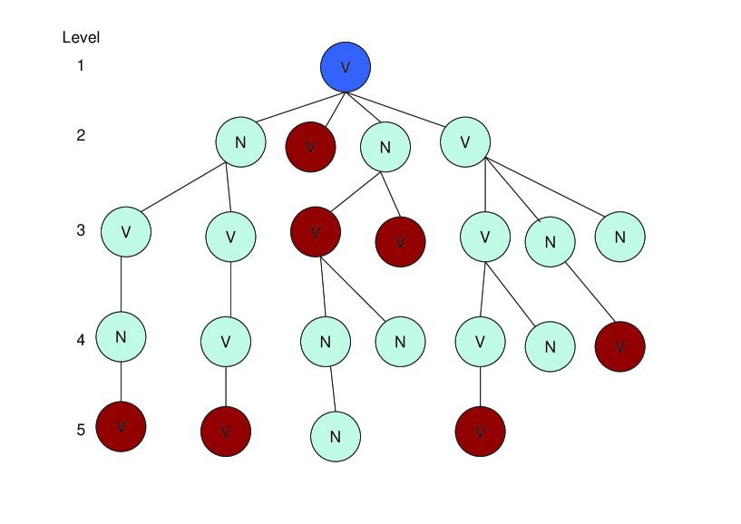
Figure 1: Example of the HiFOF algorithm is illustrated with a five-level hierarchical tree structure of one FOF halo. Points with ”V” stand for ”virialized” halos whereas points with ”N” are for ”unvirialized” halos. Blue, brown, and light-blue points represent the FOF halo, the selected galactic subhalos, and the subhalos dropped. As mentioned in the text, the hierarchical tree is constructed through the FOF method with gradually reduced linking lengths. To determine whether a subhalo is bound, the virial condition of it is checked. We start with selecting the samples from virialized subhalos on the highest level; once a member in a branch is selected, others in that branch will be discarded. We then move to the next lower level and repeat the procedures just described. A completed subhalo sample is then acquired after every level is examined.

Additionally, unlike the unbound procedure that iteratively removes the unbound particles with the greatest energy until only bound particles remain in the subhalo (Springel et al., 2001a), our subhalos are treated as a whole and can not be separated into bound and unbound particles. In other words, if a subhalo can not pass the virial condition check, we will drop it entirely. After the virial conditions of all subhalos in the tree are checked, the virialized subhalos on every branch at the highest possible level are then selected to be the samples used in our analysis; other unvirialized subhalos and virialized subhalos not at the highest possible level are dropped. Figure 1 schematically shows how the HiFOF algorithm works. Continuing the same procedure on all FOF halos, subhalo samples are then constructed. This full subhalo sample is also called the HiFOF sample in this study.

Figure 2 shows the cumulative mass functions of (bright and dark) subhalos for the four simulations at redshifts $z=0$ (left) at $z=1$ (right). The densities are $7.11\times 10^{-2}~{}h^{3}~{}Mpc^{-3}$ ($\Lambda CDM_{100a}$), $7.33\times 10^{-2}~{}h^{3}~{}Mpc^{-3}$ ($\Lambda CDM_{200}$), $1.53\times 10^{-1}~{}h^{3}~{}Mpc^{-3}$ ($\Lambda CDM_{100b}$), $1.53\times 10^{-1}~{}h^{3}~{}Mpc^{-3}$ ($\Lambda CDM_{100c}$), and $4.37\times 10^{-1}~{}h^{3}~{}Mpc^{-3}$ (${}^{*}\Lambda CDM_{100c}$) at $z=0$. The accumulated subhalo mass functions in our simulations basically are consistent with each other. In other words, at the same redshift the mass function is mildly dependent on the box size and the mass resolution. However, it is observed that the rapid increase appears at the low mass end and is possibly due to the resolution effect when different resolution runs are compared. At $z=1$, the four simulations agree with each other to a lesser degree. It indicates that the difference likely arises from the different softening-length adopted as well as from sample variance.

2.3 Galaxy Model

Galaxy formation involves complicated processes. Despite that, cooling is essential to lower the specific entropy in the gas, thereby increasing the gas density. Bremsstrahlung and line coolings are the most efficient cooling mechanisms for this purpose (e.g., Kaze et al., 1996). However, these cooling mechanisms require the gas temperature to be above or close to the ionization temperature. When a self-gravitating gas is cooled, it can also be heated by adiabatic contraction. It is thus possible for the gas to maintain a temperature above the threshold cooling temperature during the contraction, thereby yielding to cooling runaway to form stars. In our galaxy model, we hence demand that the host halo potential must be sufficiently deep for the gas to get above the ionization temperature. This condition is translated to a threshold host halo mass, only above which stars can form within the host halo.

Now, consider a halo with a virial mass $M$ and a virial radius $R$, $M$ can be related to $R$ as

$$M=\frac{4\pi}{3}\rho_{vir}R^{3}=\frac{4\pi}{3}\Delta_{c}(z)\rho_{bg}R^{3},$$ (2)

where $\rho_{vir}$ is the virial density, $\Delta_{c}(z)$ the mean overdensity of spherically virialized objects formed at redshift $z$, and $\rho_{bg}$ the background density $\equiv\rho_{0}(1+z)^{3}$. The overdensity $\Delta_{c}(z)$ at each redshift can be evaluated using a fitting formula by Kitayama & Suto (1996). For example, $\Delta_{c}\approx 335$ at $z=0$ and $\Delta_{c}\approx 201$ at $z=1$ for our cosmology, $\Omega_{0}=0.3$ and $\Omega_{\Lambda}=0.7$.

In order to facilitate efficient gas cooling, a deep gravitational potential is needed for the virial temperature to exceed roughly the ionization temperature, i.e. $kT_{vir}~{}_{\sim}^{>}~{}\frac{b}{2}\alpha^{2}m_{e}c^{2}$, where $\alpha$ is the fine structure constant, $m_{e}$ the electron mass, and $c$ the speed of light, and $b$ has is a fudge factor of order unity. The virial temperature for a star-forming halo can be obtained as

$$kT_{vir}\approx\frac{GMm_{p}}{5R}\gtrsim\frac{b}{2}\alpha^{2}m_{e}c^{2}$$ (3)

where G is the gravitational constant, k the Boltzmann constant, and $m_{p}$ the proton mass. Using Equation (2) to replace $R$ by $M$, it follows that

$$M\gtrsim M_{c}\approx(\frac{(\frac{5b}{2}(\frac{3}{4\pi})^{1/3}\alpha^{2}m_{e}c^{2})}{(\Delta_{c}(z)\rho_{bg})^{1/3}Gm_{p}})^{3/2}$$

$$\approx 7.0\times 10^{12}~{}(\Delta_{c}(z)(1+z)^{3})^{-1/2}~{}h^{-1}~{}M_{\odot},$$ (4)

where a value of $b\approx 0.8$ has been adopted. At $z=0$, the threshold halo mass $M_{c}\approx 4.0\times 10^{11}~{}h^{-1}~{}M_{\odot}$. We apply the mass threshold to select those FOF halos, which host our galaxy samples. All other subhalos hosted by less massive FOF halos are considered dark, void of star formation.

3 Simulation Results and Observations

In this section we will compare our galaxy samples with the observed galaxies. Comparisons include the differential mass function, the galaxy number density evolution, the two point correlation function at low and high redshifts, the halo occupation distribution, and finally the kinetic pair fraction.

3.1 Differential Mass Function

Luminosity function (LF for short) $\phi(L)$ gives the relative numbers of galaxies of different luminosities, and is so defined that $\phi(L)dL$ is the number of galaxies in the luminosity interval $L\rightarrow L+dL$ per unit volume of the Universe. The luminosity function of galaxies can be fitted by Schechter’s (1976) formula,

$$\phi(L)dL=\phi^{\star}(\frac{L}{L_{\star}})^{\alpha}exp(\frac{-L}{L_{\star}})\frac{dL}{L_{\star}}.$$ (5)

We adopt $\phi^{\star}=(26.39^{+1.81}_{-1.62})\times 10^{-4}$ $Mpc^{-3}$, $\alpha=-1.30$, and $L_{\star}=10^{(-(M^{\star}+M_{\odot B})/2.5)}L_{\odot}=1.987\pm 0.25\times 10^{10}L_{\odot}$ for $M^{\star}=-21.07\pm 0.13$ from DEEP2 B-band galaxies at $z\sim 0.3$ (Faber et al., 2007) for comparison later in our analysis. The mass function and luminosity function are related by $F(M)dM=\phi(L)dL$. If L can be expressed as a function of M when there is no scatter between $M$ and $L$, the mass function $F(M)$ can be derived from the luminosity function $\phi(L)$. Hoekstra et al. (2005) measured the weak-lensing signal as a function of rest-frame B-, V-, and R-band luminosities for a sample of “isolated” galaxies from the Red-Sequence Cluster Survey with photometric redshifts $0.2<z<0.4$. They fit the measurements with a power-law for the mass-to-light ratio

$$M=M_{fid}(\frac{L}{10^{10}h^{-2}L_{\odot}})^{\beta},$$ (6)

where $M_{fid}$ is the virial mass of a fiducial galaxy of luminosity $L=10^{10}$ $h^{-2}L_{x,\odot}$, and x indicates the relevant filter. In B band, they obtained $M_{fid}=9.9^{+1.5}_{-1.3}\times$ $10^{11}~{}h^{-1}~{}M_{\odot}$ and $\beta=1.5\pm 0.3$. With the power law form of the mass-to-light ratio, $F(M)$ can be found as follows,

$$F(M)=\frac{\phi^{\star}(10^{10})^{\alpha+1}}{L_{\star}^{\alpha+1}\beta M_{fid}}\times(\frac{M}{M_{fid}})^{\frac{\alpha+1}{\beta}-1}\times\exp^{-(\frac{M}{M_{fid}})^{1/\beta}\frac{10^{10}}{L_{\star}}}.$$ (7)

However, the galaxy mass measured by the weak lensing signal may in fact not represent the true galaxy mass correctly. Notably, the weak lensing mass may include the mass of the host halo (FOF halo) of an isolated galaxy. We select those from our sample galaxies with only a single HiFOF subhalo residing in an FOF halo in our simulations, i.e. the isolated galaxy, to suit the observation requirement. These subhalos are a small population of the entire galaxy sample and are used as a mass calibrator. The ratios of the selected isolated galaxies to the whole galaxy sample are 32% for $\Lambda CDM_{100a}$, 16% for $\Lambda CDM_{100b}$, 27% for $\Lambda CDM_{200}$, and 12% for $\Lambda CDM_{100c}$. The result is shown in Figure 3 and the 1 $\sigma$ error bars are plotted only for $\Lambda CDM_{100b}$. It is found that the relation reveals a power-law form. The power law form follows

$$log_{10}(M_{g})=a*loh_{10}(M_{h})+b,$$ (8)

where $a=1.00621$ and $b=-0.806326$ for the average on all simulations. Extrapolating this power law relation to smaller galaxy mass subhalos, we apply this relation to our entire galaxy samples.

Figure 4 shows differential mass functions derived from the luminosity function and the M/L relation in Equation (7) and our galaxy samples at $z=0.3$ after applying the $M_{g}-M_{h}$ power law relation in Figure 3 to our galaxy samples. The mass functions of four simulations agree with the observation, and also with each other, quite well. In highest mass range, $M>10^{13}~{}h^{-1}~{}M_{\odot}$, and in the low mass end, the profiles of our mass functions show the excess compared with the observational data.

In order to understand the low mass excess, a galaxy mass cut with $n_{min}=10$ denoted as ${}^{*}\Lambda CDM_{100c}$, in contrast to $n_{min}=30$ for $\Lambda CDM_{100c}$, is analyzed. We find that the low-mass excess is pushed toward lower mass. Hence, it is expected that the low-mass excess can be pushed to the very low mass end if the simulation mass resolution approaches infinitely high. As for the high-mass excess, it is likely related to the over-abundance of CD galaxies at the cluster centers, whose population deviates from the Schechter’s function.

3.2 Galaxy Density Evolution

As the high redshift data are gradually gathered in recent years, study of galaxy properties in time evolution becomes feasible. An aspect to test our galaxy model is to make comparison with the observed galaxy density evolution. When we integrate Equation (5) over luminosity, it gives the galaxy number density,

$$n_{(>L)}=\int^{\infty}_{L}\Phi(L^{\prime})dL^{\prime}.$$ (9)

That is, with given $\phi^{\star}$, $\alpha$, $L_{\star}$, and a luminosity cut $L$, the galaxy number density can be obtained. It is suggested by Conroy et al. (2005) that isolated galaxies at $z\sim 1$ have a similar mass as isolated galaxies that are 1 mag fainter at $z\sim 0$. They found that there has been little or no evolution in the halo mass of isolated galaxies with magnitudes in the range $\sim M_{B}^{\star}-0.5~{}to~{}-1.5$, even though $M_{B}^{\star}$ has evolved by $\sim 1$ mag over this redshift range. This result is adopted in our analysis. However, Conroy et al. (2005) also assume that there is no evolution for isolated galaxies with magnitudes $\sim M_{B}^{\star}+2.5\log_{10}4$, which is equivalent to $L_{\star}/4$. The luminosity cut $L$ in Equation (9) for $n_{(>L)}$ is set to be greater than $L_{\star}(z)/4$. That is, the cut is $L_{\star}(z)$-dependent. In contrast, we need to find the corresponding redshift-independent mass-cut from the simulations to make a correct comparison if the previous result and the assumption are to be adopted. Unlike others using the galaxy density as an indicator to provide a certain absolute magnitude threshold so as to determine the galaxy mass, we take a different approach. We combine the LF of the DEEP2 B-band galaxies and the mass-to-light relation at $z\sim 0.3$, as well as the $M_{g}-M_{h}$ relation discussed in Section 3.1 to obtain the corresponding mass-cut. The luminosity cut of $L_{\star}(z\sim 0.3)/4$ given from the observed DEEP2 LF is then converted to a galaxy mass-cut in our samples with $7.02\times 10^{10}~{}h^{-1}~{}M_{\odot}$ in the $\Lambda CDM_{100a}$, $7.06\times 10^{10}~{}h^{-1}~{}M_{\odot}$ in the $\Lambda CDM_{200}$, $7.01\times 10^{10}~{}h^{-1}~{}M_{\odot}$ in the $\Lambda CDM_{100b}$ , $6.66\times 10^{10}~{}h^{-1}~{}M_{\odot}$ in the $\Lambda CDM_{100c}$, and $5.79\times 10^{10}~{}h^{-1}~{}M_{\odot}$ in the ${}^{*}\Lambda CDM_{100c}$. The mass cut is applied to all redshift and the redshift evolution of the galaxy number density can then be obtained for our galaxy samples.

Figure 5 presents the number density evolution of our data and the observed galaxy density data by integrating the luminosity functions (Equation 9) of  Faber et al. (2007), which include measurements of Combo-17 (Faber et al., 2007), FDF (Gabasch et al., 2004), Bell SDSS (Bell et al., 2003), VVDS (Ilbert et al., 2005), 2df (Norberg et al., 2002), DEEP2 (Faber et al., 2007), and SDSS (Blanton et al., 2003). The profiles of our galaxy density are basically in broad agreement with the observed galaxies. Our data show the same evolutionary trend, a decline with the redshift. However, at low redshift, a depletion is found in our simulations. The depletion can probably be attributed to the failure of the assumption for the redshift-independent mass-cut at low redshift, and can be corrected if a different mass-cut at low redshift is assumed.

3.3 Two-Point Correlation Function

The two-point correlation function $\xi(r)$ (CF for short) is the most used indicator to quantify the degree of clustering in a galaxy sample. It is defined as a measure of the excess probability above Poisson for finding an objects in a volume element $dV$ at a separation $r$ from an otherwise randomly chosen object,

$$dP=n[1+\xi(r)]dV,$$ (10)

where $n$ is the mean number density of the object in question. It follows a simple power law form,

$$\xi(r)=(\frac{r}{r_{0}})^{-\gamma},$$ (11)

where $r_{0}$ is the correlation length and $\gamma$ is the power index of CF.

To learn about the real-space correlation function, we follow the standard practice and compute the projected correlation function

$$w_{p}(r_{p})=2~{}\int^{r_{max}}_{0}\xi(\sqrt{r_{p}^{2}+y^{2}})dy.$$ (12)

The integration limit $r_{max}$ is set to be $40~{}h^{-1}~{}Mpc$ for $z$ = 0 as in SDSS samples. The projected correlation functions of our galaxy samples at $z=0$ are shown in Figure 6. The solid line represents the volume limited sample ($M_{r}<-19.0$) of SDSS galaxy (Zehavi et al., 2005) with the density $1.507\times 10^{-2}~{}h^{3}~{}Mpc^{-3}$, $r_{0}=4.56\pm 0.23~{}h^{-1}~{}Mpc$, and $\gamma=1.89\pm 0.03$. We select the mass cuts for our galaxy samples to match the number density of SDSS. It is seen that both the amplitude and shape of the projected CF at $z=0$ are in very good agreement with those of the SDSS data for all simulations. The close agreement of galaxy correlation functions implies that the overall clustering of the galaxy population is determined by the distribution of their dark matter subhalos subject to the condition of a sufficiently deep halo potential to trigger galaxy formation. In Figure 7 we plot the galaxy-galaxy CFs $\xi(r)_{gg}$ and the subhalo-subhalo CFs $\xi(r)_{hh}$ without imposing the condition of a sufficiently deep host halo potential for comparison. It clearly shows that $\xi(r)_{hh}$ also obeys a power law form, but with a flatter slope and a smaller amplitude. Note that the number density of the subhalo sample that gives $\xi(r)_{hh}$ is roughly 5 times higher than that of our galaxy subhalos for all simulations.

Figure 8 shows the results of the projected correlation functions at $z=1$ of our galaxy samples for the four simulations and the volume-limited sample of bright, $(M_{B}\geq-19.0)$, DEEP2 galaxies (Coil et al., 2006). The upper integration limit is set to $r_{max}=20~{}h^{-1}~{}Mpc$ in our simulations to agree with the DEEP2 samples. The DEEP2 galaxy sample has a density of $1.3\times 10^{-2}~{}h^{3}~{}Mpc^{-3}$. We therefore select our samples to match the density of the DEEP2 sample. In Figure 8, it can be seen that the correlation functions of the DEEP2 galaxies and our samples also agree very well.

In Figure 9 and Figure 10, the correlation length $r_{0}$ and the power index $\gamma$ are plotted as a function of different space density at $z=0$ and $z=1$, respectively. The CFs are fit over the range of scales from 0.2 to $13~{}h^{-1}~{}Mpc$ where the errors in $\xi(r)$ in our samples are the ”jackknife” 1 $\sigma$ errors, computed using the eight octants of the simulation cube (see Weinberg et al., 2004). Figure 9 is basically adopted from Figure 11 in Kravtsov et al. (2004) which includes the Two-Degree Field (2dF; Norberg et al., 2002), SDSS galaxy surveys (Zehavi et al., 2002; Budavari et al., 2003) and their simulation data. We additionally add the newest SDSS data (Zehavi et al., 2005) and our galaxy data into Figure 9. The strong dependence of correlation length $r_{0}$ on the number density $n$ is evident in Figure 9. That is, brighter galaxies are more clustered. In addition, a nearly constant profile of $\gamma$ in observations is seen. The amplitude of $\gamma$ in our simulations, in general, also presents a roughly flat trend although at $n\approx 10^{-2}~{}h^{3}~{}Mpc^{-3}$ our $n$ values show slight depletion compared with the observations. At $z=1$ we plot the DEEP2 data released by Coil et al. (2006), the simulation results of Kravtsov et al. (2004), and our data. A similar conclusion as at $z=0$ is obtained for $r_{0}$, and our values of $\gamma$ also show good consistency with the DEEP2 galaxies.

3.4 Halo Occupation Distribution (HOD)

The HOD formalism, developed during the last several years, has become a powerful theoretical framework for predicting and interpreting galaxy clustering. The original HOD uses the probability $P(N|M)$ to describe the bias of a class of galaxies that a halo of virial mass M contains N such galaxies.  Berlind et al. (2003) studied HOD and found that at a given halo mass it is statistically independent of the halo s large-scale environment. In addition, they compared HOD of a semi-analytic model and of gasdynamics simulations in detail and concluded that the semi-analytical HOD for samples of the same space density agree remarkably well with simulations, despite that the two methods predict different galaxy mass functions.

Kravtsov et al. (2004) showed that HOD can actually be understood as a combination of the probability for a halo of mass M to host a central galaxy and the probability to host a number of satellite galaxies that obeys Poisson statistics. We analyze the first moment of HOD, $\langle N(M_{h})\rangle\equiv\langle N_{c}(M_{h})\rangle+\langle N_{s}(M_{h})\rangle$, as a function of host mass $M_{h}$ for the halo samples, where $\langle N_{c}\rangle$ is the HOD of central galaxies modeled as a step function $\langle N_{c}\rangle=1$ for $M>M_{min}$ and $\langle N_{c}\rangle=0$ otherwise, and $\langle N_{s}\rangle$ is number of the satellite galaxies modeled as a power law $\langle N_{s}\rangle\propto M^{\alpha}$ suggested by Kravtsov et al. (2004). Zehavi et al. (2005) used this HOD framework to interpret their results. Due to a finite (but important) subset of information encoded in the correlation function for galaxy clustering, a restricted HOD model was employed and fitted with a small number of free parameters. The HOD formulation they implemented has three free parameters: $M_{min}$, the minimum halo mass for galaxies above the luminosity threshold, $M_{1}$, the mass of a halo hosting one satellite galaxy above the luminosity threshold, and $\alpha$, the power law slope of the satellite mean occupation function. They took $M_{min}$ to be fixed by matching the observed space density of the sample, leaving $M_{1}$ and $\alpha$ as free parameters to fit their projected CFs. More recently, Zheng et al. (2007) modeled the luminosity-dependent projected two-point correlation function of DEEP2 $(z\sim 1)$ and SDSS $(z\sim 0)$ galaxies within the HOD framework. They adopted a more flexible parameterizations with five parameters, motivated by the less satisfactory results of Zheng et al. (2005) as well as of the three-parameter parameterizations. In the following test on this aspect, only the three-parameter parametrization scheme is adopted for simplicity.

We compute the HOD of our galaxy samples to obtain $M_{min}$, $M_{1}$, and $\alpha$ as a function of galaxy number density to make comparisons with SDSS and DEEP2 galaxies. In Figure 11$(a)$, from top to bottom, our results of $M_{min}$, $M_{1}$, and $\alpha$ in the four simulations at $z=0$ and those of SDSS galaxies are compared. It can be seen that $M_{min}$ and $M_{1}$ of four simulations not only agree with each other, implying the lesser degree of dependence on the box size and the resolution, but also match the observation quite well no matter in the magnitude or in the trend. Despite the increasing trend of the slope $\alpha$ with a decreasing density is similar to that of SDSS galaxies, the $\alpha$ value of our HODs on the whole appears to be slightly smaller than that of the observations. This may results in slightly insufficient subhalos found in massive clusters in our samples. Figure 11$(b)$ shows our results at $z=1$ and the observational data of DEEP2 galaxies. As on can see, the agreements on $M_{min}$, $M_{1}$, and $\alpha$ are also good.

3.5 Pair Fraction

Since our galaxy sample can well reproduce the observed evolution of galaxy number density, the mass function, the 2-point correlation function and the HOD, we therefore make an attempt to put another comparison to the simulation resolution limit by exploring the pair fraction and merger rate.

DEEP2 Team  (Lin et al., 2004) explored the kinematic close pair fraction and the merger rate up to redshift $z\sim 1.2$ and disclosed weak evolution in the galaxy pair fraction. Assuming mild luminosity evolution, they found the number of companions per luminous galaxy to evolve as $(1+z)^{m}$, with m = 0.51 $\pm$ 0.28 for the $r_{max}=50~{}h^{-1}~{}kpc$ case. Recently,  Lin et al. (2008) used more complete data to study the same problem, and obtained an improved result with m = 0.41 $\pm$ 0.20 for all galaxies. These two studies consistently reveal that the pair fraction of galaxies indeed undergo weak evolution.

We study the pair fraction problem with our galaxy samples; our approach is in variance with applying a ”hybrid” formalism to address this problem (Berrier et al., 2006), which combines an N-body simulation to account for large-scale structure and the host dark matter halo population and an analytic substructure model (Zentner et al., 2005) to identify satellite galaxies within the host halos. We test our samples with the same setup as in Lin et al. (2004) and Lin et al. (2008). They defined close pairs such that the projected separations satisfy $10~{}h^{-1}~{}kpc$ $\leq$ $\Delta r$ $\leq$ $r_{max}$, where $r_{max}$ = 30, 50, or 100$~{}h^{-1}~{}kpc$, and the rest-frame relative velocity $\Delta v$ less than 500 $km~{}s^{-1}$. To ensure the selection of the same types of galaxies at different redshifts in the presence of luminosity evolution, a specific range in the evolution-corrected absolute magnitude $M^{e}_{B}$, defined as $M_{B}+Qz$, was adopted in our analysis where the evolution is parameterized as $M(z)=M(z=0)-Qz$. Lin et al. (2008) adopted $Q=1.3$ found by Faber et al. (2007) and restricted their analysis to galaxies with luminosities $-21\leq M^{e}_{B}\leq-19$ for $z$ = 0.45-1.2. Applying the mass-to-light ratio in Equation (6) for B-band with $M_{fid}=9.9^{+1.5}_{-1.3}\times$ $10^{11}~{}h^{-1}~{}M_{\odot}$ and $\beta=1.5\pm 0.3$, we are able to convert the mass to the luminosity. The luminosity range, $-21.39$ $\leq M_{B}\leq$ $-19.39$, at $z=0.3$ is considered because the mass-to-light ratio data of Hoekstra et al. (2005) was collected at an average redshift $z\sim 0.3$. The mass range at $z=0.3$ after conversion is found to be $2.38\times 10^{11}~{}h^{-1}~{}M_{\odot}$ $\leq M\leq$ $3.78\times 10^{12}~{}h^{-1}~{}M_{\odot}$. Moreover, the average number of companions per galaxy is defined as

$$N_{c}\equiv\frac{2N_{p}}{N_{g}},$$ (13)

where $N_{p}$ is the number density of individual paired galaxies and $N_{g}$ the number density of galaxies as suggested in Berrier et al. (2006). Following Berrier et al. (2006), we also adopt a fiducial relative line-of-sight velocity difference of $|\Delta v|=500$ $km~{}s^{-1}$. A close-pair cylinder volume is then constructed by a constant $\Delta v$ cut. In our analysis, only the $r_{max}$ = 50, and $100~{}h^{-1}~{}kpc$ cases are considered due to the limitation of our mass resolution.

Figure 12 shows the redshift $z$ versus the pair fraction for $r_{max}$ = 50 (bottom) and $r_{max}$ = $100~{}h^{-1}~{}kpc$ (top). The pair fraction data are taken from Lin et al. (2004) including SSRS2 (da Costa et al., 1998), CNOC2 (Yee et al., 2000), and DEEP2 early data (Davis et al., 2003) and from full samples in Lin et al. (2008) including SRSS2, CNOC2, MGC (Millennium Galaxy Catalog, Liske et al., 2003; Driver et al., 2005; Allen et al., 2006), TKRS (Wirth et al., 2004), and DEEP2 (Davis et al., 2003, 2007). Our data points are consistent with the DEEP2 medium to high redshift observations although at low redshift we have lower values than other observations. However, the mild evolution trend is seen. Using the fitting formula, $N_{c}(0)(1+z)^{m}$, proposed in Lin et al. (2004) and Lin et al. (2008), we find the following results. For $r_{max}=50~{}h^{-1}~{}kpc$ , $N_{c}(0)=0.036$ and $m=1.17$ in the $\Lambda$$CDM_{100a}$ , $N_{c}(0)=0.074$ and $m=1.07$ in the $\Lambda$$CDM_{200}$, $N_{c}(0)=0.046$ and $m=0.96$ in the $\Lambda$$CDM_{100b}$, $N_{c}(0)=0.025$ and $m=1.43$ in the $\Lambda$$CDM_{100c}$, and $N_{c}(0)=0.028$ and $m=1.37$ in the ${}^{*}\Lambda$$CDM_{100c}$. For $r_{max}=100~{}h^{-1}~{}kpc$, $N_{c}(0)=0.137$ and $m=0.65$ in the $\Lambda$$CDM_{100a}$, $N_{c}(0)=0.207$ and $m=0.95$ in the $\Lambda$$CDM_{200}$, $N_{c}(0)=0.182$ and $m=0.48$ in the $\Lambda$$CDM_{100b}$, $N_{c}(0)=0.107$ and $m=0.98$ in the $\Lambda$$CDM_{100c}$, and $N_{c}(0)=0.116$ and $m=0.92$ in the ${}^{*}\Lambda$$CDM_{100c}$. Apparently, our pair fractions show stronger evolution than those in Lin et al. (2004) and Lin et al. (2008), where $m=0.51\pm 0.28$ and $m=0.41\pm 0.14$ for $r_{max}$ = $50~{}h^{-1}~{}kpc$, and $m=0.47\pm 0.18$ and $m=0.29\pm 0.05$ for $r_{max}$ = $100~{}h^{-1}~{}kpc$, but appear to agree with the results of Berrier et al. (2006) for $r_{max}$ = $50~{}h^{-1}~{}kpc$, where $m=0.42\pm 0.17$ for $V_{now}$, the maximum circular velocity of the subhalo at the current epoch, and $m=0.99\pm 0.14$ for $V_{in}$, the maximum circular velocity of the subhalo when it was first accreted into the host halo.

The steeper slope in our sample is rooted on the too-low galaxy density at low $z$, which can basically be attributed to the failure of our assumption on the redshift-independent mass-cut. We note that the pair fraction critically depends on the galaxy density and the density is determined by the luminosity cut. Consequently, if a wrong luminosity evolution assumption is adopted, this can lead to a high galaxy mass-cut, a lower galaxy density, and finally a lower pair fraction. Our data at low redshift reveal this effect and result in a steeper slope.

4 Conclusion and Discussion

In this study we have used the HiFOF method to locate and identify subhalos, and we advance the idea that galaxies form only in a sufficiently massive halo due to its sufficiently high gas cooling efficiency. It is estimated that the threshold halo mass $M_{c}\approx 4.0\times 10^{11}$ $h^{-1}M_{\odot}$ at $z=0$, and our galaxy samples are constructed from the HiFOF subhalos embedded in the halos satisfying this mass threshold. There are far more subhalos that are hosted by halos not meeting the mass threshold. They are dark halos where star formation cannot occur. To test our model, we have analyzed the differential mass function, two-point correlation function (CF), the space density evolution, the HOD, and the pair fraction from our galaxy samples. The results are summarized as follows.

(1) Combing the luminosity function (LF) and the mass to light relation (M/L), a differential mass function can be derived. Based on the lensing signal from Red-Sequence Cluster Survey to determine the galaxy mass, we have corrected the lensing mass in our galaxy samples so as to make fair comparison. We find that the mass functions of our four simulations agree with the LF and M/L data very well.

(2) We compare our galaxy density evolution with the evolution of the observational galaxy number density through the integration of a LF with a proper luminosity cut. Our simulations basically show fair consistency with observations, except at low-redshift. The insufficient density is likely due to the failure of the assumption at low redshift about the redshift-independent mass-cut. The depletion in the galaxy number density also reflects a similar result in pair fractions found at low-redshift.

(3) We have analyzed CFs of our galaxy subhalos at $z=0$ and at $z=1$. At $z=0$, we select our galaxies to have the density $1.507\times 10^{-2}~{}h^{3}~{}Mpc^{-3}$ to make comparison with the volume limited sample ($M_{r}<-19$) of SDSS galaxies. Both the slope and the amplitude are consistent with the SDSS. At $z=1$, we select samples at $n=1.3\times 10^{-2}~{}h^{3}~{}Mpc^{-3}$ to setup the same density condition as in the volume-limited sample of bright (corrected), $M_{B}>-19.0$, DEEP2 galaxies. The projected correlation functions are compared, and our profiles are similar to the one found in DEEP2 galaxies.

(4) We also study $r_{0}$ and $\gamma$ as a function of the space density $n$. Our galaxies reveal the increase of $r_{0}$ as $n$ decreases, a similar result also found in the observation data. In other words, the correlation length $r_{0}$ has luminosity dependence, and the brighter the galaxies, the larger the correlation length. On the other hand, the power index $\gamma$ of observation data displays a nearly constant behavior over a wide range of $n$ at $z=0$. Despite a smaller values of $\gamma$ are obtained around $n\approx 10^{-2}$ in our simulations, a roughly constant trend on the whole is seen. The same results are reached at $z=1$ as well.

(5) We have parameterized our HODs with three parameters $M_{1}$, $M_{min}$, and $\alpha$ as a function of the galaxy number density. Our values of $M_{1}$ and $M_{min}$ and their increasing trend as the galaxy density decreases show good agreement with SDSS data (Zehavi et al., 2005; Zheng et al., 2007) and DEEP2 data (Zheng et al., 2007), and the depletion of the slope $\alpha$ at $z=0$ may be attributed to insufficient subhalos found in massive clusters.

(6) We have analyzed the kinematic pair fraction of our galaxy samples by selecting the mass in between $2.28\times 10^{11}~{}h^{-1}~{}M_{\odot}$ and $3.61\times 10^{12}~{}h^{-1}~{}M_{\odot}$ which are obtained by applying the observed mass-to-light ratio to convert the luminosity range $-21.39$ $\leq M_{B}^{e}\leq$ $-19.39$ at $z=0.3$. Parameterizing the evolution of the pair fraction as $(1+z)^{m}$, Lin et al. (2008) find that when $r_{max}=50$ $~{}h^{-1}~{}kpc$, $m=0.41\pm 0.14$ for the full sample. We obtain $m=1.17$ in $\Lambda CDM_{100a}$, $m=1.07$ in $\Lambda CDM_{200}$, $m=0.96$ in $\Lambda CDM_{100b}$, $m=1.43$ in $\Lambda CDM_{100c}$, and $m=1.37$ in ${}^{*}\Lambda CDM_{100c}$. When $r_{max}=100~{}h^{-1}~{}kpc$, in contrast to $0.29\pm 0.05$ found by Lin et al. (2008), we find $m=0.65$ in $\Lambda CDM_{100a}$, $m=0.95$ in $\Lambda CDM_{200}$, $m=0.48$ in $\Lambda CDM_{100b}$, $m=0.98$ in $\Lambda CDM_{100c}$ and $m=0.92$ in ${}^{*}\Lambda CDM_{100c}$. The steeper slope basically results from insufficient close pairs found at low redshift, which is interpreted as the deficient low-$z$ galaxy density in our samples due to the failure of the assumption on the redshift-independent mass-cut. However, the situation is less severe for the $r_{max}=100~{}h^{-1}~{}kpc$ case where milder evolution trend is more evident.

Most of the above tests for our galaxy samples provide supporting evidence for our galaxy model. However, this model has some problems of its own. First, this model does not provide information of the galaxy morphology. Second, unlike the Millennium simulation (Springel et al., 2005), this model does not contain any empirical ingredient to trace individual galaxy evolution.

The solution to the first problem requires the gas component to be included in the simulation, which can reveal the amount of residual gas angular momentum in the subhalo thereby providing additional information of morphological types. The complexity of the second problem is intractable from the first-principle calculations and it needs an empirical model, much as what was added to the Millennium, to approximate the physics involved.

We would like to thank Lihwai Lin and Tak-Pong Woo for many helpful discussions and suggestions. This project is supported in part by the grant: NSC-92-2628-M-002-008-MY3 (1/3).

Figure 2: Cumulative mass functions of (bright and dark) subhalo samples obtained in our analysis at redshift z = 0 (left panel) in the $\Lambda CDM_{100a}$ (solid line), $\Lambda CDM_{200}$ (long-dashed line) , $\Lambda CDM_{100b}$ (short-dashed line) , and $\Lambda CDM_{100c}$ (dotted line) and at $z$ = 1 (right panel). The mass range plotted are down to the minimum mass of $4.1\times 10^{10}~{}h^{-1}~{}M_{\odot}$ in the $\Lambda CDM_{100a}$ and $\Lambda CDM_{200}$, to that of $1.9\times 10^{10}~{}h^{-1}~{}M_{\odot}$ in the $\Lambda CDM_{100b}$, to that of $1.52\times 10^{10}~{}h^{-1}~{}M_{\odot}$ in the $\Lambda CDM_{100c}$, and to that of $5.16\times 10^{9}~{}h^{-1}~{}M_{\odot}$ in the ${}^{*}\Lambda CDM_{100c}$. These mass functions are generally consistent with each other. As a result, we believe that the influence of the box size and resolution effect are not important for our HiFOF samples.

Figure 3: Diagram shows $M_{h}$ (Mass of the isolated FOF halos) vs. $M_{g}$ (Mass of the HiFOF identified subhalos) at redshift $z\sim 0.3$. As shown in the figure, the relation can be approximated as a power law. This power law is used to provide the correction on galaxy mass from the weak lensing mass. The error bars represent 1 $\sigma$ values, and similar bars also exist for other curves, but omitted for the clarity of presentation.

Figure 4: Differential mass functions at redshift $z=0.3$ of LF + M/L data (solid line), the $\Lambda CDM_{100a}$ samples (long-dashed line), $\Lambda CDM_{200}$ (short-dashed line) , $\Lambda CDM_{100b}$ (dotted line), $\Lambda CDM_{100c}$ dashed-dotted line) , and ${}^{*}\Lambda CDM_{100c}$ (short-dashed dotted line). The mass of our galaxy samples is modified according to the relation in Fig 3. We list the space density as follows. The number density $n=2.01\times 10^{-2}~{}h^{3}~{}Mpc^{-3}$ in $\Lambda CDM_{100a}$, $2.11\times 10^{-2}~{}h^{3}~{}Mpc^{-3}$ in $\Lambda CDM_{200}$, $3.22\times 10^{-2}~{}h^{3}~{}Mpc^{-3}$ in $\Lambda CDM_{100b}$, $2.82\times 10^{-2}~{}h^{3}~{}Mpc^{-3}$ in $\Lambda CDM_{100c}$, and $4.77\times 10^{-2}~{}h^{3}~{}Mpc^{-3}$ in ${}^{*}\Lambda CDM_{100c}$. Our data profiles are similar to the observational data line despite deviations shown in the two ends, the lower and higher mass range.

Figure 5: Galaxy density as a function of the redshift is plotted. Observational data are based on the data of the LFs in  Faber et al. (2007) and can be converted to the galaxy density evolution by using Equation (9). A proper luminosity cut, $L\geq L_{\star}(z)/4$, is adopted for the density calculation, and combining the data of the DEEP2 B-band galaxies and the mass-to-light relation at $z~{}\sim 0.3$, as well as the $M_{g}-M_{h}$ relation, a corresponding mass-cut can be obtained and then applied to galaxy samples at other redshifts to obtain $n(z)$.

Figure 6: Projected correlation functions of the galaxy samples at $z=0$ in the $\Lambda CDM_{100a}$ (dashed line), $\Lambda CDM_{200}$ (dotted line), $\Lambda CDM_{100b}$ (open triangle with the error bar), and $\Lambda CDM_{100c}$ (dashed-dotted line) are compared with the projected correlation function of the volume limited sample ($M_{r}<-19$) of the SDSS galaxy (Zehavi et al., 2005) with the density $1.507\times 10^{-2}~{}h^{3}~{}Mpc^{-3}$.

Figure 7: The correlation functions $\xi(r)_{gg}$ of the galaxy samples at $z=0$ in the $\Lambda CDM_{100a}$ (solid line), $\Lambda CDM_{200}$ (dashed line), $\Lambda CDM_{100b}$ (short-dashed line), and $\Lambda CDM_{100c}$ (dotted line) are plotted. In contrast, the subhalo-subhalo projected correlation $\xi(r)_{hh}$ is presented with $\#$. It is clearly shown that $\xi(r)_{hh}$ obeys a power law form, but with a flatter slope and a smaller amplitude. That is, our galaxy samples behaves substantially differently from HiFOF samples.

Figure 8: Comparison of the projected correlation functions between our four simulations at $z=1$ and the DEEP2 volume limited data of bright, $M_{B}<-19.0$, galaxies (Coil et al., 2006). The CF of the DEEP2 data has a density $0.013~{}h^{3}~{}Mpc^{-3}$. We therefore select our samples to have the same density, and the results can be found to be in good agreement with the DEEP2 data.

Figure 9: Top: Best-fit correlation scale $r_{0}$ as a function of number density at the present-day epoch. Bottom: Best-fit slope $\gamma$ of the correlation function as a function of number density. This plot is based on the Figure 11 in Kravtsov et al. (2004) plus the newest SDSS data (Zehavi et al., 2005) and our data. Our values of the correlation length $r_{0}$ are consistent with observational data. The values of the power index $\gamma$ are lower at density around $n=10^{-2}~{}h^{3}~{}Mpc^{-3}$. However, the agreement between observations and our data is seen.

Figure 10: Same as Figure 9, but for $z=1$. We additionally include DEEP2 data released by (Coil et al., 2006) as well as our data. It is found that the correlation length and the power index in our simulations match DEEP2 data well.

Figure 11: From top to bottom, the three fitting parameters $M_{1}$, $M_{min}$, and $\alpha$ of the HOD formulation are plotted as a function of the galaxy number density $n_{g}$. In 11(a), the open circles represent SDSS data (Zehavi et al., 2005) and the stars with errorbars give also SDSS data (Zheng et al., 2007), and in 11(b) the stars with errorbars give DEEP2 data (Zheng et al., 2007), while the filled square, circle, triangle, diamond, and pentagon are for the $\Lambda CDM_{100a}$, $\Lambda CDM_{200}$, $\Lambda CDM_{100b}$, $\Lambda CDM_{100c}$, and ${}^{*}\Lambda CDM_{100c}$ data. Consistency between SDSS galaxies and our galaxy samples is observed at $z=0$. The good agreements are also seen between DEEP2 galaxies and ours at $z=1$.

Figure 12: Pair fraction, $N_{c}$, as a function of redshift z. The crosses mark the results from DEEP2 early data (2003). The open squares represents measurements from SSRS2, MGC, and CNOC2. The open circles show DEEP2 data (2007). The open triangles are from TKRS. The stars, filled squares, circles, triangles, and diamonds give our simulation results from $\Lambda CDM_{100a}$, $\Lambda CDM_{200}$, $\Lambda CDM_{100b}$, $\Lambda CDM_{100c}$, and ${}^{*}\Lambda CDM_{100c}$. Two cases of $r_{max}$, 50 (bottom) and 100 (top) $~{}h^{-1}~{}kpc$, are considered.

Table 1: Simulation Parameters

	$L_{Box}$	$N_{dm}$	$M_{dm}$	$\epsilon_{z=0}$	$\sigma_{8}$
Name	($h^{-1}~{}Mpc)$		($h^{-1}~{}M_{\odot})$	($~{}h^{-1}~{}kpc$)
$\Lambda$$CDM_{100a}$	100	$256^{3}$	4.125 $\times 10^{9}$	6.0	0.94
$\Lambda$$CDM_{200}$	200	$512^{3}$	4.125 $\times 10^{9}$	10.0	0.94
$\Lambda$$CDM_{100b}$	100	$512^{3}$	6.188 $\times 10^{8}$	3.0	0.94
$\Lambda$$CDM_{100c}$	100	$512^{3}$	5.156 $\times 10^{8}$	10.0	0.94

References

- Allen et al. (2006) Allen, P. D., Driver, S. P., Graham, A. W., Cameron, E., Liske, J. & de Propris, R. 2006, MNRAS, 371, 2
- Bell et al. (2003) Bell, E. F., McIntosh, D. H., Katz, N. & Weinberg, M. D. 2003, ApJS, 149, 289
- Berlind et al. (2003) Berlind, A. A. et al. 2003, ApJ, 593, 1
- Berrier et al. (2006) Berrier, J. C., Bullock, J. S., Barton, E. J., Guenther, H. D., Zentner, A. R., & Wechsler, R. H. 2006, ApJ, 652, 56
- Blanton et al. (2003) Blanton, M. R. et al. 2003, ApJ, 592, 819
- Budavari et al. (2003) Budavari, T. et al. 2003, ApJ, 595, 59
- Coil et al. (2006) Coil, A. L., Newman, J. A., Cooper, M. C., Davis, M., Faber, S. M., Koo, D. C., & Willmer, C. N. 2006, ApJ, 644, 671
- Conroy et al. (2005) Conroy, C. et al. 2005, ApJ, 635, 982
- Conroy et al. (2006) Conroy, C., Wechsler, R., Kravtsov, A. 2006, ApJ, 647, 201
- da Costa et al. (1998) da Costa, L. N. et al. 1998, AJ, 116, 1
- Davis et al. (1985) Davis, M., Efstathiou, G., S., Frenk, C. S., & White, S. D. M. 1985, ApJ, 292, 371
- Davis et al. (2003) Davis, M. et al. 2003, SPIE, 4834, 161
- Davis et al. (2007) Davis, M. et al. 2007, ApJ, 660, L1
- Driver et al. (2005) Driver, S. P., Liske, J., Cross, N. J. G., De Propris, R., & Allen, P. D. 2005, MNRAS, 360, 81
- Faber et al. (2007) Faber, S. M. et al. 2007, ApJ, 665, 265
- Gabasch et al. (2004) Gabasch, A. et al. 2004, A&A, 412, 41
- Hoekstra et al. (2005) Hoekstra, H., Hsieh, B. C., Yee, H. K. C., Lin, H., & Gladders, M. D. 2005, ApJ, 635, 73
- Ilbert et al. (2005) Ilbert, O. et al. 2005, A&A, 439, 863
- Kaze et al. (1996) Katz, Neal, Weinberg, David H., Hernquist, Lars, Miralda-Escude, Jordi 1996, ApJ, 457, L57
- Kitayama & Suto (1996) Kitayama, Tetsu, Suto, Yashshi 1996, ApJ, 469, 480
- Klypin et al. (1999) Klypin, A., GottlAober, S., & Kravsov, A. V. 1999, ApJ, 516, 530
- Kravtsov et al. (2004) Kravtsov, A. V., Berlind, A. A., Wechsler, R. H., Klypin, A. A., Gottloeber, S., Allgood, B., & Primack, J. R. 2004, ApJ, 609, 35
- Lin et al. (2004) Lin, L. et al. 2004, ApJ, 617, L9
- Lin et al. (2008) Lin, L. et al. 2008, ApJ, 681, 232
- Liske et al. (2003) Liske, J., Lemon, D. J., Driver, S. P., Cross, N. J. G., & Couch, W. J. 2003, MNRAS, 344, 307
- Neyrinck et al. (2004) Neyrinck, M. C., Hamilton, A. J. S., & Gnedin, N. Y. 2004, MNRAS, 348, 1
- Norberg et al. (2002) Norberg, P. et al. 2002, MNRAS, 332, 827
- Riess et al. (1998) Riess, A. G. et al. 1998, AJ, 116, 1009
- Sanchez et al. (2006) Sanchez, A. G., Baugh, C. M., Percival, W. J., Peacock, J. A., Padilla, N. D., Cole, S., Frenk, C. S., & Norberg, P. 2006, MNRAS, 336, 189
- Seljak et al. (2005) Seljak, U. et al. 2005, Phys. Rev. D, 71, 103515
- Spergel et al. (2003) Spergel, D. N. et al. 2003, ApJS, 148, 175
- Springel (2005) Springel, V. 2005, MNRAS, 364, 1105
- Springel et al. (2005) Springel, V. et al. 2005, Nature, 435, 629
- Springel et al. (2001a) Springel, V., White, S. D. M., Tormen, G., & KauRmann, G. 2001a, MNRAS, 328, 726
- Springel et al. (2001b) Springel, V., Yoshidaa, N., & White, S. D. 2001b, New Astronomy, 6, 79
- Stadel et al. (1997) Stadel, J., Katz, N., Weinberg, D. H., & Hernquist, L. 1997, SKID
- Tegmark et al. (2004) Tegmark, M. et al. 2004, ApJ, 606, 702
- Weinberg et al. (2004) Weinberg, D. H., Dave, R., Katz, N., & Hernquist, L. 2004, ApJ, 601, 1
- White et al. (1993) White, S. D. M., Navarro, J. F., Evrard, A. E., & Frenk, C. S. 1993, Nature, 336, 429
- Wirth et al. (2004) Wirth, G. D. et al. 2004, AJ, 127, 3121
- Yee et al. (2000) Yee, H. K. C. et al. 2000, ApJS, 129, 475
- Zehavi et al. (2002) Zehavi, I. et al. 2002, ApJ, 571, 172
- Zehavi et al. (2005) Zehavi, I. et al. 2005, ApJ, 630, 1
- Zentner et al. (2005) Zentner, A. R., Berlind, A. A., Bullock, J. S., Kravtsov, A. V., & Wechsler, R. H. 2005, ApJ, 624, 505
- Zheng et al. (2005) Zheng, Z. et al. 2005, ApJ, 633, 791
- Zheng et al. (2007) Zheng, Z., Coil, A. L., Zehavi, I. 2007, ApJ, 667, 760