Cosmology with Unparticles

Abstract

We discuss cosmological consequences of the existence of physics beyond the standard model that exhibits Banks-Zaks and unparticle behavior in the UV and IR respectively. We first derive the equation of state for unparticles and use it to obtain the temperature dependence of the corresponding energy and entropy densities. We then formulate the Boltzmann and Kubo equations for both the unparticles and the Banks-Zaks particles, and use these results to determine the equilibrium conditions between the standard model and the new physics. We conclude by obtaining the constraints on the effective number of degrees of freedom of unparticles imposed by Big-Bang nucleosynthesis.

I Introduction

Recently Georgi Georgi:2007ek ; Georgi:2007si raised the interesting possibility that physics beyond the Standard Model (SM) may contain a sector that is conformally invariant in the IR region (guaranteed by a zero of the beta function), and classically scale-invariant in the UV; we refer to these as the unparticle (${\cal U}$) and Banks-Zaks (${{\cal B}{\cal Z}}$) phases, respectively. The transition region between the two phases is characterized by the scale of dimensional transmutation $\Lambda_{\cal U}$ A specific realization of this idea can be found in Banks:1981nn ; following this reference we will assume that the new sector is described as an asymptotically free gauge theory in the ${{\cal B}{\cal Z}}$ phase.

This novel idea has received substantial attention within the high-energy community, mainly in connection with the phenomenology of such models. Here we discuss some fundamental issues in the evolution of the Universe in the presence of this type of new physics (though studies of the cosmological consequences of the proposal have appeared in the literature  Davoudiasl:2007jr -Kikuchi:2007az , these publications ignore several essential aspects which are discussed below). In sec. II we derive an approximate equation of state for the NP sector. Then, in sec. III we use this together with the expected SM-NP interactions Georgi:2007ek ; Georgi:2007si to determine the conditions under which the SM and NP sectors were in equilibrium. In sec. IV, using the experimental constraints derived from Big-Bang Nucleosynthesis (BBN) we obtain non-trivial bounds on the parameters of the theory. The Appendices A and B are devoted to presentation of two alternative derivation of the Boltzmann equation.

II Thermodynamics of unparticles

In order to understand the thermodynamic behavior of the new sector  we use the expression for the trace anomaly of the energy momentum tensor of a gauge theory where all the renormalized masses vanish Collins:1976yq :

$$\theta_{\mu}^{\mu}=\frac{\beta}{2g}N\left[F^{\mu\nu}_{a}F_{a\;\mu\nu}\right]\,,$$ (1)

where $\beta$ denotes the beta function for the coupling $g$ and $N$ stands for the normal product.

The basic assumption for the unparticle phase is that the $\beta$ function has a non-trivial IR fixed point at $g=g_{\star}\not=0$. Modeling the unparticle sector by a gauge theory, we assume that for low temperatures 

$$\beta=a(g-g_{\star}),\quad a>0\,,$$ (2)

in which case the running coupling reads

$$g(\mu)=g_{\star}+u\mu^{a};\qquad\beta[g(\mu)]=au\mu^{a}\,,$$ (3)

where $u$ is an integration constant and $\mu$ is the renormalization scale.

We look for the lowest-order corrections to the conformal limit (where $\theta^{\mu}_{\mu}=0$) when the system is in thermal equilibrium at temperature $T$, is isotropic and homogeneous, and does not have any net conserved charge. Since $\beta$ vanishes in the conformal limit, in (1) we can take $\left\langle N\left[F^{\mu\nu}_{a}F_{a\;\mu\nu}\right]\right\rangle$ equal to its conformal value (we denote the thermal average by $\left\langle\cdots\right\rangle$); taking the renormalization scale $\mu=T$ we then expect

$$\left\langle N\left[F^{\mu\nu}_{a}F_{a\;\mu\nu}\right]\right\rangle=bT^{4+\gamma}\,,$$ (4)

where $\gamma$ is the anomalous dimension of the operator. Using $\left\langle\theta_{\mu}^{\mu}\right\rangle=\rho_{\cal U}-3P_{\cal U}$, where $\rho_{\cal U}$ and $P_{\cal U}$ denote the energy density and pressure of the unparticle phase, together with (3) and (4) then gives

$$\rho_{\cal U}-3P_{\cal U}=AT^{4+\delta};\quad\left(A\equiv\frac{aub}{2g_{\star}},~{}\delta\equiv a+\gamma\right)\,,$$ (5)

where we took $\mu=T$.

Combining (5) with the thermodynamic relation $d(\rho V)+P\;dV=T\;d(sV)$ ($s$ is the entropy density), when $\rho$ and $P$ are functions of $T$ only, and integrating, we find,

$$\rho_{\cal U} = \sigma T^{4}+A\left(1+\frac{3}{\delta}\right)T^{4+\delta}$$ (6)

$$P_{\cal U} = \frac{1}{3}\sigma T^{4}+\left(\frac{A}{\delta}\right)T^{4+\delta}$$ (7)

$$s_{\cal U} = \frac{4}{3}\sigma T^{3}+A\left(1+\frac{4}{\delta}\right)T^{3+\delta}$$ (8)

where $\sigma$ is an integration constant and we assumed $\delta\not=0$.

It is worth noticing that the terms $\propto A$ correspond to deviations from the standard relativistic relation $V\propto T^{-3}$. The behavior at low temperatures depends on the sign of $\delta$, we will assume $\delta>0$. Then

$$3P_{\cal U}=\rho_{\cal U}\left[1-B\rho_{\cal U}^{\delta/4}\right];\quad B=\frac{A}{\sigma^{1+\delta/4}}$$ (9)

exhibiting the lowest-order corrections to the often-used expression $P=w\rho$, $w=$const. This effect might be of interest in the discussion of the possible dark-energy effects contained in this model, but will not be discussed here.

Elucidating the cosmological effects of the modified equation of state (8) lies beyond the scope of the present paper, we merely remark that the NP increases the coefficient of the $T^{4}$ term in $\rho$ and induces $O(T^{\delta})$ corrections; e.g. in the radiation-dominated era the scale parameter behaves as $(1+cT^{\delta})^{1/3}/T$ ($c=$const.).

In general we expect $A\propto\Lambda_{\cal U}^{-\delta}$ since $\Lambda_{\cal U}$ is the scale associated with broken scale invariance; then the energy density for the new sector in the unparticle phase equals

$$\rho_{\cal U}=\frac{3}{\pi^{2}}T^{4}\left[g_{\rm IR}+\left(\frac{T}{\Lambda_{\cal U}}\right)^{\delta}f\right];\qquad T\ll\Lambda_{\cal U}$$ (10)

where we replaced $\sigma=3g_{\rm IR}/\pi^{2}$ (hereafter we use the normalization from Maxwell-Boltzmann statistics) and $g_{\rm IR}$, the effective number of relativistic degrees of freedom (RDF), will be estimated below.

In the ${{\cal B}{\cal Z}}$ phase we assume the theory is asymptotically free so that, up to logarithmic corrections,

$$\rho_{{\cal B}{\cal Z}}=\frac{3}{\pi^{2}}g_{{\cal B}{\cal Z}}T^{4};\qquad T\gg\Lambda_{\cal U}$$ (11)

where $g_{{\cal B}{\cal Z}}$ denotes the RDF in this phase.

For intermediate temperatures the explicit form of the thermodynamic functions requires a complete non-perturbative calculation and the choice of a specific model; fortunately we will not need to consider the detailed behavior of the system. Given that $\rho\propto T^{4}$ in both the IR and UV regions, for our purposes it will be sufficient to use the interpolation

$$\rho_{\rm NP}\equiv\frac{3}{\pi^{2}}g_{\rm NP}T^{4};\quad g_{\rm NP}=g_{{\cal B}{\cal Z}}\theta(T-\Lambda_{\cal U})+g_{{\cal U}}\theta(\Lambda_{\cal U}-T)$$ (12)

where $g_{{\cal U}}=[g_{\rm IR}+\left(T/\Lambda_{\cal U}\right)^{\delta}f]$ while NP stands for ‘new physics’; $g_{\rm NP}$ will be continuous at $T=\Lambda_{\cal U}$ when $f=g_{{\cal B}{\cal Z}}-g_{\rm IR}$, which we now assume. It is worth noting that a mass distribution of unparticles with the spectral density $\propto(\mu^{2})^{(d_{\cal U}-2)}$ Georgi:2007ek generates the term $\propto f$ in (12) with $\delta=2(d_{\cal U}-1)$, assuming that the contributions with $\mu>T$ decouple. We emphasize that (12) will be used only as a rough but convenient approximation that reproduces the expected behavior at low and high temperatures. In cases of interest we expect $g_{\rm IR}\sim g_{{\cal B}{\cal Z}}\gg f$ so that the terms $\propto T^{\delta}$ are subdominant.

Estimating $g_{\rm IR}$ directly form the model Lagrangian is a non-trivial exercise, due to the expected strong-coupling nature of the theory in the infrared. Using, however, the AdS-CFT correspondence Gubser:1999vj we find

$$g_{\rm IR}=\frac{\pi^{5}}{8}(LM_{Pl})^{2}$$ (13)

where $L$ denotes the AdS radius of curvature and $M_{Pl}$ is the Planck mass. Given that $L$ is expected Gubser:1999vj to be significantly smaller than $1/M_{Pl}$, it is justified to expect that

$$g_{\rm IR}\,{\raise-3.0pt\hbox{$\sim$}}\!\!\!\!\!{\raise 2.0pt\hbox{$>$}}\,{\cal O}(100)$$ (14)

In the following we will use this as our estimate for the RDF in the unparticle phase.

In order to estimate $g_{{\cal B}{\cal Z}}$ one must specify the details of the non-Abelian theory in the ultraviolet regime. For the models considered in Banks:1981nn we find

$$g_{{\cal B}{\cal Z}}\sim 100$$ (15)

This result is based on a model for which the couping constant stays within the perturbative regime throughout its evolution. There is also non-perturbative lattice evidence Svetitsky:2009pz that gauge theories exhibiting an infrared fixed point obey (15). In the following we will adopt this estimate.

The energy density $\rho_{\cal U}$ was also discussed in Chen:2007qc , however the expression presented in this reference agrees with (10) only when $g_{\rm IR}=0$ and therefore does not include the leading low-temperature behavior of the theory.

III SM-NP interactions and equilibrium

The presence of a NP sector of the type considered here can have important cosmological consequences since, even when weakly coupled to the SM, its energy density will affect the expansion rate of the universe; this can then be used to obtain useful limits on the effective number of degrees of freedom $g_{\rm NP}$. This calculation requires a determination of the relationship between the temperature of the NP and SM sectors to which we now turn.

The interactions we will consider have the generic form

$${\cal L}_{\rm int}=\epsilon{\cal O}_{\rm SM}{\cal O}_{\rm NP}$$ (16)

where the first term is a gauge invariant operator composed of SM fields (possible Lorentz indices have been suppressed), while the second operator is either composed of ${{\cal B}{\cal Z}}$ fields or is an unparticle operator, depending on the relevant phase of the NP sector. The coupling $\epsilon$ in general has dimensions and is assumed to be small. For the specific calculations presented below we will assume for simplicity that ${\cal O}_{{\rm SM},{\rm NP}}$ are both scalar operators.

Leading interactions involve SM operators that can generate 2 particle states since states with higher particle number will be phase-space suppressed. From such interactions we obtain the NP$\leftrightarrow$SM reaction rate $\Gamma$, which will be precisely defined below. The two sectors will then be in equilibrium whenever $\Gamma\,{\raise-3.0pt\hbox{$\sim$}}\!\!\!\!\!{\raise 2.0pt\hbox{$>$}}\,H$, where $H$ denotes the Hubble parameter Kolb , and decouple at the transition temperature $T_{f}$:

$$T=T_{f}:~{}\Gamma\simeq H;\quad H^{2}=\frac{8\pi}{3M_{Pl}^{2}}\rho_{\rm tot};$$ (17)

where

$$\rho_{\rm tot} = \rho_{\rm SM}+\rho_{\rm NP}$$ (18)

$$= \frac{3}{\pi^{2}}\left(g_{\rm SM}T_{\rm SM}^{4}+g_{\rm NP}T_{\rm NP}^{4}\right)$$ (19)

We denote by $T_{\rm SM}$ and $T_{\rm NP}$ the temperatures for the SM and NP sectors which can be different when these sectors are not in equilibrium

The approach to equilibrium can be described using either the Kubo formalism (appendix A) or a suitable extension of the Boltzmann equation formalism (appendix B). It follows form the expressions derived in the appendices that the conditions near equilibrium are determined by the equation

$$\dot{\vartheta}+4H\vartheta=-\Gamma\vartheta;\;\;\;\;\vartheta=T_{\rm NP}-T_{\rm SM}$$ (20)

where, using the Kubo formalism,

$$\Gamma = \frac{\pi^{2}}{12T^{4}}\left(\frac{1}{g_{\rm SM}}+\frac{1}{g_{\rm NP}}\right)\epsilon^{2}\Re\left\{\int_{0}^{\beta}ds\int_{0}^{\infty}dt\int d^{3}{\bf x}\;\left\langle{\cal O}_{\rm SM}(-is,{\bf x})\dot{\cal O}_{\rm SM}(t,{\bf 0})\right\rangle\left\langle{\cal O}_{\rm NP}(-is,{\bf x})\dot{\cal O}_{\rm NP}(t,{\bf 0})\right\rangle\right\}$$ (21)

The Boltzmann equation (BE) calculation also yields (20) with the rate given by

$$\Gamma=\frac{\pi^{2}}{12T^{3}}\left(\frac{1}{g_{\rm SM}}+\frac{1}{g_{\rm NP}}\right)\frac{1}{2T}\sum_{X^{\prime},X}\int d\Phi_{\rm NP}d\Phi_{\rm SM}\beta(E_{\rm SM}-E_{\rm SM}^{\prime})^{2}e^{-\beta E_{\rm SM}}\left|{\cal M}\right|^{2}(2\pi)^{4}\delta(K_{\rm SM}-K_{\rm NP})$$ (22)

where ${\cal M}$ is the matrix element (with no spin averaging) derived form the SM-NP interaction Lagrangian , $E_{\rm SM}$ and $E_{\rm SM}^{\prime}$ denote the initial and final energies of the Standard Model particles in the reaction, and $K_{{\rm SM},{\rm NP}}$ the total 4-momenta of each sector for the reaction; we have also assumed the Boltzmann approximation (neglecting Pauli blocking or Bose-Einstein enhancement) and denoted by $d\Phi_{\rm SM,NP}$ the appropriate phase-space measures (without any spin factors). In particular, for the unparticle phase we use Georgi:2007ek

$$d\Phi_{\cal U}=A_{d_{\cal U}}\epsilon(q^{0})\;\theta(q^{2})\;(q^{2})^{d_{\cal U}-2}\frac{d^{4}q}{(2\pi)^{4}}$$ (23)

where $A_{n}=(4\pi)^{3-2n}/[2\Gamma(n)\Gamma(n-1)]$. We show in appendix B that (21) and (22) are, in fact, equal.

The solutions to (20) yields $\rho\propto R^{-4}$ in the absence of the collision term (proportional to $\Gamma$), as expected for a scale invariant theory. It is also important to note that, in contrast to other authors (Davoudiasl:2007jr -Lewis:2007ss ), (22) contains an unparticle-decay term (see appendix B), as we find the arguments (based on the deconstruction picture Stephanov:2007ry ) for neglecting these contributions unjustified.

The detailed calculation of $\Gamma$ requires a specific form of the interaction ${\cal O}_{\rm SM}{\cal O}_{\rm NP}$ (see above for a specific example). However for the purposes of the remaining calculations only the basic properties of $\Gamma$, such as its dependence on $T$ and the relevant RDF will be needed. These properties can be obtained using dimensional analysis: if the dimensions of the operators are, respectively $d_{\rm SM}$ and $d_{\rm NP}$ and if the number of degrees of freedom involved in this interaction are $g_{\rm SM}^{\prime}$ and $g_{\rm NP}^{\prime}$, then, including a phase-space factor we find

$$\Gamma\sim\frac{\epsilon^{2}\lambda g_{\rm tot}}{(4\pi)^{n_{\rm SM}+n_{\rm NP}-1}}T^{2d_{\rm SM}+2d_{\rm NP}-7};\quad\lambda\equiv\frac{g_{\rm SM}^{\prime}}{g_{\rm SM}}\frac{g_{\rm NP}^{\prime}}{g_{\rm NP}}\,,$$ (24)

where $n_{\rm SM}$ and $n_{\rm NP}$ denote numbers of SM and NP fields in the corresponding operators; in the unparticle phase we take $g_{\rm NP}^{\prime}=d_{\cal U}$ and $n_{\rm NP}=2(d_{\cal U}-1)$, where $d_{\cal U}$ denotes the dimension of ${\cal O}_{\cal U}$.

The value of $\lambda$ depends on the details of the model. Above the Higgs ($\phi$) mass $m_{\phi}$ (we assume $m_{\phi}\sim v\equiv\left\langle\phi\right\rangle$) the most important operator is ${\cal O}_{\rm SM}=\phi^{\dagger}\phi$; in this case $g_{\rm SM}^{\prime}=4$, so $\lambda\sim(4/g_{\rm SM})\cdot(g_{\rm NP}^{\prime}/g_{\rm NP})$. Below $m_{\phi}$ there are many dimension 4 SM operators relevant for the SM-NP equilibration, e.g. $\bar{\ell}\phi e$ (containing an extra suppression by the factor $\sim v/M_{\cal U}$; $\ell,e$ denote a lepton isodoublet and isosinglet respectively), or $B_{\mu\nu}B^{\mu\nu}$ (where $B$ is the hypercharge gauge field), in this case we expect $g_{\rm SM}^{\prime}\sim g_{\rm SM}$, so that $\lambda\sim g_{\rm NP}^{\prime}/g_{\rm NP}$.

III.1 The Banks-Zaks phase.

We will assume that the ${{\cal B}{\cal Z}}$ sector corresponds to an $SU(n_{c})$ Yang-Mills theory with $n_{f}$ vector-like massless fermions in the fundamental representation (denoted by $q_{{\cal B}{\cal Z}}$). Assuming that $\Lambda_{\cal U}>v$, the leading SM$\leftrightarrow$NP interaction is of the form

$${\cal L}=\frac{1}{M_{\cal U}}\left(\phi^{\dagger}\phi\right)\left(\bar{q}_{{{\cal B}{\cal Z}}}q_{{{\cal B}{\cal Z}}}\right)$$ (25)

where we assume that all flavors in the ${{\cal B}{\cal Z}}$ sector couple with the same strength. In this case ($\epsilon=1/M_{\cal U}$)

$$\Gamma_{{\cal B}{\cal Z}}\simeq\frac{\lambda g_{\rm tot}}{(4\pi)^{3}M_{\cal U}^{2}}T^{3}$$ (26)

Denoting by $T_{{{\cal B}{\cal Z}}\hbox{\tiny-}f}$ the solution to (17) when $\Gamma$ is given by (26), and imposing also the consistency conditions $M_{\cal U}>T_{{{\cal B}{\cal Z}}\hbox{\tiny-}f}>\Lambda_{\cal U}$, we obtain ( $g_{\rm tot}$ is evaluated at $T_{{{\cal B}{\cal Z}}\hbox{\tiny-}f}$)

$$1>\frac{T_{{{\cal B}{\cal Z}}\hbox{\tiny-}f}}{M_{\cal U}}=\frac{\sqrt{(8\pi)^{5}g_{\rm tot}}}{\lambda g_{\rm tot}}\;\frac{M_{\cal U}}{M_{Pl}}>\frac{\Lambda_{\cal U}}{M_{\cal U}}$$ (27)

III.2 The unparticle phase.

In this case we will consider only interactions of the form Georgi:2007ek ($k=d_{\rm SM}+{d_{{\cal B}{\cal Z}}}-4$)

$${\cal L}=\frac{\Lambda_{\cal U}^{{d_{{\cal B}{\cal Z}}}-d_{\cal U}}}{M_{\cal U}^{k}}{\cal O}_{\rm SM}{\cal O}_{\cal U}$$ (28)

Using (24) we obtain (here we use $n_{\rm NP}=2(d_{\cal U}-1)$)

$$\Gamma_{\cal U}\sim\frac{\lambda g_{\rm tot}\Lambda_{\cal U}}{(4\pi)^{n_{\rm SM}+2d_{\cal U}-3}}\left(\frac{\Lambda_{\cal U}}{M_{\cal U}}\right)^{2k}\left(\frac{T}{\Lambda_{\cal U}}\right)^{2d_{\rm SM}+2d_{\cal U}-7}$$ (29)

Denoting by $T_{{\cal U}\hbox{\tiny-}f}$ the solution to (17) when $\Gamma$ is given by (29), and imposing also the consistency condition $\Lambda_{\cal U}>T_{{\cal U}\hbox{\tiny-}f}$, we obtain (here $g_{\rm tot}$ is evaluated at $T_{{\cal U}\hbox{\tiny-}f}$)

$$\frac{T_{{\cal U}\hbox{\tiny-}f}}{\Lambda_{\cal U}}=\left[\frac{(4\pi)^{n_{\rm SM}+2d_{\cal U}-3}}{\lambda\sqrt{\pi g_{\rm tot}/8}}\frac{\Lambda_{\cal U}}{M_{Pl}}\left(\frac{M_{\cal U}}{\Lambda_{\cal U}}\right)^{2k}\right]^{1/(2d_{\rm SM}+2d_{\cal U}-9)}<1$$ (30)

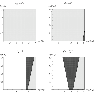
Figure 1: Regions in the $\Lambda_{\cal U}-M_{\cal U}$ plane corresponding to various freeze-out and thaw-in scenarios for $d_{\cal U}=3/2,~{}2,~{}3,~{}7/2$. Dark grey: SM-NP decoupling in the unparticle phase only; light grey: no SM-NP decoupling; in the white regions $T_{{\cal U}\hbox{\tiny-}f}<v$ ($\Lambda_{\cal U},~{}M_{\cal U}$ are in TeV units). We assumed $g_{\rm SM}=g_{{\cal B}{\cal Z}}=g_{{\cal U}}=100$, $g_{\rm SM}^{\prime}=4$, $g_{{\cal B}{\cal Z}}^{\prime}=50$ and $g_{{\cal U}}^{\prime}=d_{\cal U}$. For the ${{\cal B}{\cal Z}}$ phase: $n_{SM}=n_{NP}=2$, $d_{\rm SM}=2$ and $d_{NP}=3$, while for the ${\cal U}$ phase: $n_{SM}=2$, $n_{NP}=2(d_{\cal U}-1)$, $d_{\rm SM}=2$ and $d_{NP}=d_{\cal U}$.

For $d_{\cal U}<4.5-d_{\rm SM}$, $\Gamma/H$ has the singular property of increasing as $T$ drops, whence SM and NP will equilibrate for $T<T_{{\cal U}\hbox{\tiny-}f}$ (thaw-in); due to the constraints  on $d_{\cal U}$ ($d_{\cal U}<1$ is excluded  Grinstein:2008qk ) this can only happen for ${\cal O}_{\rm SM}=\phi^{\dagger}\phi$. The opposite occurs if $d_{\cal U}>4.5-d_{\rm SM}$ (freeze-out). For $d_{\cal U}=4.5-d_{\rm SM}$, the approximations (19), (24) are insufficient and a detailed calculation is required to determine freeze-out and/or thaw-in conditions; we will not consider this special case further.

There are various possible scenarios for decoupling of the NP sector. The situation in the very early Universe ($T>M_{\cal U}$) depends on the UV completion (including the mediator interactions) of the NP and will not be considered here. If (27) holds then we have a standard freeze-out scenario: the SM and NP sectors will be in equilibrium down to $T\sim T_{{{\cal B}{\cal Z}}\hbox{\tiny-}f}$ and decouple below this value; thereafter the two sectors evolve keeping their entropies separately conserved. Since no mass thresholds or phase transitions are crossed  the SM and NP temperatures remain equal down to $T\sim\Lambda_{\cal U}$.

The situation for $\Lambda_{\cal U}\,{\raise-3.0pt\hbox{$\sim$}}\!\!\!\!\!{\raise 2.0pt\hbox{$>$}}\,T$ is more complicated. If (30) holds (which defines a region in the $\Lambda_{\cal U}-M_{\cal U}$ plane), decoupling occurs in the unparticle phase. For $T>v$ the most relevant operator is ${\cal O}_{\rm SM}=\phi^{\dagger}\phi$, and both thaw-in (for $d_{\cal U}<2.5$) and freeze-out (for $d_{\cal U}>2.5$) may be present. For $v>T$ all the relevant SM operators have $d_{\rm SM}=4$, and only freeze-out is possible; in this case $T_{{\cal U}\hbox{\tiny-}f}$ may be significantly smaller than $v$.

Other parameter values lead to more complicated scenarios, e.g. a double decoupling: freeze-out in the ${{\cal B}{\cal Z}}$, thaw-in in the unparticle phase and then freeze out below $v$. In spite of the many possibilities, there is always a temperature below which the SM and NP decouple.

In Fig. 1 we show regions in the $(\Lambda_{\cal U},M_{\cal U})$ space that correspond to various freeze-out and thaw-in scenarios for a reasonable parameter choice. For this calculation we assumed that ${\cal O}_{\rm SM}=\phi^{\dagger}\phi$ is responsible for maintaining the equilibrium between the SM and NP (so $d_{\rm SM}=2$). For consistency that choice implied an additional constraint $T_{{\cal U}\hbox{\tiny-}f}>v$ (below $v$ other SM operators are relevant). For interactions with the ${{\cal B}{\cal Z}}$ phase an operator $\propto(\phi^{\dagger}\phi)(\bar{q}_{{{\cal B}{\cal Z}}}q_{{{\cal B}{\cal Z}}})$, was adopted (in which case ${d_{{\cal B}{\cal Z}}}=3$).

IV Big Bang Nucleosynthesis

The light-element abundances resulting from BBN are sensitive to the expansion rate that determines the temperature of the universe (see e.g. Iocco:2008va ), which can be used to restrict possible additional RDF, or, in our case, $g_{\rm IR}$. We express our results in terms of the number of extra neutrino species, $\Delta N_{\nu}$, defined through

$$\rho_{\rm NP}=\frac{3}{\pi^{2}}\frac{7}{4}\left(\frac{4}{11}\right)^{4/3}\Delta N_{\nu}T_{\gamma}^{4}\,,$$ (31)

which is valid for $T$ below the $e^{+}e^{-}$ annihilation ($T_{\gamma}$ stands for the photon temperature). For $\Delta N_{\nu}$ we adopt the recent bounds obtained in Iocco:2008va : $\Delta N_{\nu}=0.0\pm 0.3_{\rm stat}(2\sigma)\pm 0.3_{\rm syst}$.

We first consider the case where SM and NP were in equilibrium down to a temperature $T_{f}>v$, and decoupled thereafter. Then the entropy conservation for the NP and SM sectors implies

$$g_{\rm NP}^{\star}(T_{f})(T_{f}R_{f})^{3} = g_{\rm NP}^{\star}(T_{\rm NP})(T_{\rm NP}R)^{3}$$ (32)

$$g_{\rm SM}^{\star}(T_{f})(T_{f}R_{f})^{3} = g_{\rm SM}^{\star}(T_{\gamma})(T_{\gamma}R)^{3}$$ (33)

where $R_{f}$ is the scale factor at the decoupling while $R$ corresponds to temperature of photons $T_{\gamma}$ ($T_{\rm NP}$ is the corresponding NP temperature); $g_{\rm NP}^{\star}$ and $g_{\rm SM}^{\star}$ stand for the NP and SM effective numbers of RDF conventionally Kolb adopted for the entropy density. After $e^{+}e^{-}$ annihilation neutrinos and photons generate the dominant SM contribution, but their temperatures differ. Using standard expressions Kolb we find

$$g_{\rm SM}^{\star}(T_{\gamma})=g_{\gamma}\frac{g_{\gamma}+g_{e}+g_{\nu}}{g_{\gamma}+g_{e}}\,,$$ (34)

where $g_{i}$ stands for the number of RDF corresponding to the species $i$. Assuming that $g_{\rm NP}$ is almost constant in the temperature range we are interested in and neglecting possible right-handed neutrino decoupling effects, the two sectors had the same temperature down to the electroweak phase transition; thereafter the temperatures split as the SM crossed its various mass thresholds and the entropy was pumped into remaining species. Entropy conservation (33) in both sectors then implies

$$T_{\rm NP}=T_{\gamma}\left[\frac{g_{\gamma}}{g_{\gamma}+g_{e}}\frac{g(\gamma,e,\nu)}{g_{\rm SM}(v)}\right]^{1/3}$$ (35)

where $g_{\rm SM}(\gamma,e,\nu)\equiv g_{\gamma}+g_{e}+g_{\nu}$, while $g_{\rm SM}(v)$ stands for the total number of SM RDF active above $T=v$. Note that the above relation holds regardless if the decoupling happened during the ${{\cal B}{\cal Z}}$ or unparticle phase. Then combining with (31) we obtain

$$g_{\rm IR}=\frac{7}{4}\left[\frac{g_{\rm SM}(v)}{g_{\rm SM}(\gamma,e,\nu)}\right]^{4/3}\Delta N_{\nu}$$ (36)

Using the standard expressions for the SM quantities Kolb the BBN constraint on $\Delta N_{\nu}$ then implies $g_{\rm IR}\,{\raise-3.0pt\hbox{$\sim$}}\!\!\!\!\!{\raise 2.0pt\hbox{$<$}}\,20$ at 95% CL. It is worth mentioning here that $\Gamma$ measures the decay rate of unparticles into SM states. After decoupling, when $\Gamma<H$ these decays become very rare (the ${\rm NP}\to{\rm SM}$ life-time becomes larger than the age of the universe $\sim 1/H$).

More severe constraints could be obtained if NP and SM remained in equilibrium down to the BBN temperature. That occurs for $\Lambda_{\cal U},~{}M_{\cal U}\sim\hbox{TeV}$ and $d_{\cal U}\sim 1$; the relevant operator being $B_{\mu\nu}B^{\mu\nu}{\cal O}_{\cal U}$. Then, since temperatures of the NP and SM sectors are the same, one obtains

$$g_{\rm IR}=\frac{7}{4}\left(\frac{g_{\gamma}}{g_{\gamma}+g_{e}}\right)^{4/3}\Delta N_{\nu}$$ (37)

which leads to $g_{\rm IR}\,{\raise-3.0pt\hbox{$\sim$}}\!\!\!\!\!{\raise 2.0pt\hbox{$<$}}\,0.25$ at 95% CL.

When decoupling occurs between $v$ and $T_{\rm BBN}$ the bound on $g_{\rm IR}$ lies between $0.25$ and $20$. When the SM and NP are never in equilibrium the BBN constraints can be used to bound $\rho_{\rm NP}$, but not $g_{\rm IR}$ since $T_{\rm NP}$ is then not known. These bounds should be compared to $g_{\rm IR}\,{\raise-3.0pt\hbox{$\sim$}}\!\!\!\!\!{\raise 2.0pt\hbox{$>$}}\,100$ typical of specific models Banks:1981nn e.g. for an ${SU(3)}$ gauge theory with $16$ fundamental fermion multiplets, and expected from AdS/CFT correspondence Gubser:1999vj . We conclude that many unparticle models will have difficulties accounting for the observed light-element abundances.

V Summary

Using the trace anomaly we argue for a form of the equation of state for unparticles that contains power-like corrections to the expression for relativistic matter; this allows us to determine temperature dependence of the energy and entropy density for unparticles. We then derive the Boltzmann equation for the ${{\cal B}{\cal Z}}$ phase and postulate a plausible form for this equation for unparticles; using this we determine the conditions for NP-SM equilibrium. Finally we derive useful constrains on the NP effective number of degrees of freedom imposed by the BBN.

Appendix A Derivation of the reaction rate using the Kubo formalism

In this section we follow closely the arguments presented in Kubo:1957mj . We consider a thermodynamic system, not necessarily in equilibrium, with macroscopic observables $\{\alpha_{i}\}$ associated with operators $\{a_{i}\}$. We assume the thermodynamics of the system is described by a density matrix $\rho$

$$\rho=\exp\left[\beta\left(\Omega-H+\sum_{i}\mu_{i}a_{i}\right)\right]$$ (38)

where the $\mu_{i}$ and $\beta$ are parameters, and $\Omega=\Omega(\mu,\beta)$ is a function chosen such that tr$\rho=1$, that is

$$e^{-\beta\Omega}={\rm Tr}e^{-\beta\left(H-\sum_{i}\mu_{i}a_{i}\right)}$$ (39)

The $\mu_{i}$ are determined by the condition

$$\alpha_{i}={\rm Tr}\rho a_{i}=-\left(\frac{\partial\Omega}{\partial\mu_{i}}\right)$$ (40)

It is important to note that $\rho$ differs from the usual grand-canonical density operator in that the $a_{i}$ are not assumed to be conserved, so the $\alpha_{i}$ will not be constant:

$$\alpha_{i}(t)={\rm Tr}\{\rho\;a_{i}(t)\}={\rm Tr}\{\rho(t)\;a_{i}\};\qquad a_{i}(t)=e^{iHt}a_{i}e^{-iHt},~{}~{}\rho(t)=e^{-iHt}\rho e^{iHt}$$ (41)

$\alpha_{i}(t)$ denotes the average of $a_{i}$ at time $t$ for a distribution for which the average of $a_{i}$ at $t=0$ is $\alpha_{i}=\alpha_{i}(0)$.

We now assume the $\mu_{i}$ are small, then a straightforward calculation yields

$$\Omega=\Omega_{0}-\sum_{i}\mu_{i}\left\langle a_{i}\right\rangle+\cdots\,,$$ (42)

where, for any operator $\xi$,

$$\left\langle\xi\right\rangle={\rm Tr}\rho_{0}\xi;\qquad\rho_{0}=e^{\beta(\Omega_{0}-H)},~{}~{}e^{-\beta\Omega_{0}}={\rm Tr}e^{-\beta H}\,.$$ (43)

Now let

$$\alpha^{\prime}_{i}(t)={\rm Tr}\rho a^{\prime}_{i}(t)={\rm Tr}\left\{\rho e^{iHt}a_{i}^{\prime}e^{-iHt}\right\}\,;\quad a_{i}^{\prime}=a_{i}-\left\langle a_{i}\right\rangle\,,$$ (44)

so that, to first order in $\mu$,

$$\alpha^{\prime}_{i}(t)=\sum_{j}\int_{0}^{\beta}ds\left\langle a^{\prime}_{j}(-is)a^{\prime}_{i}(t)\right\rangle\mu_{j}$$ (45)

Using now the cyclic property of the trace, $\left\langle\xi(z)\eta(z^{\prime})\right\rangle=\left\langle\xi(z-z^{\prime})\;\eta\right\rangle=\left\langle\xi\;\eta(z^{\prime}-z)\right\rangle$ for any operators $\xi,~{}\eta$ and any complex times $z,~{}z^{\prime}$. From this it follows that

$$\frac{d^{2}}{dt^{2}}\left\langle a^{\prime}_{i}(-is)a^{\prime}_{j}(t)\right\rangle=-\left\langle\dot{a}_{i}^{\prime}(-is)\dot{a}^{\prime}_{j}(t)\right\rangle\,,$$ (46)

hence

$$\int_{0}^{\tau}dt\left(1-\frac{t}{\tau}\right)\left\langle\dot{a}_{i}^{\prime}(-is)\dot{a}^{\prime}_{j}(t)\right\rangle=\left\langle a_{i}^{\prime}(-is)\dot{a}^{\prime}_{j}(0)\right\rangle-\frac{1}{\tau}\left[\left\langle a_{i}^{\prime}(-is)a^{\prime}_{j}(\tau)\right\rangle-\left\langle a_{i}^{\prime}(-is)a^{\prime}_{j}\right\rangle\right]\,.$$ (47)

Next, using the definition

$$\dot{\xi}(t)=i\left[H,\xi(t)\right]$$ (48)

and the cyclic property of the trace,

$$\int_{0}^{\beta}ds\left\langle a_{i}^{\prime}(-is)\dot{a}^{\prime}_{j}\right\rangle=-i\left\langle[a_{i}^{\prime},a_{j}^{\prime}]\right\rangle=-i\left\langle[a_{i},a_{j}]\right\rangle\,.$$ (49)

Collecting all results and using $\dot{a}_{i}^{\prime}=\dot{a}_{i}$,

$$\frac{\alpha^{\prime}_{i}(\tau)-\alpha^{\prime}_{i}(0)}{\tau} = -\sum_{j}{\cal G}(\tau)_{ij}\mu_{j}$$ (50)

$${\cal G}(\tau)_{ij} = \int_{0}^{\beta}ds\int_{0}^{\tau}dt\left(1-\frac{t}{\tau}\right)\left\langle\dot{a}_{j}(-is)\dot{a}_{i}(t)\right\rangle+i\left\langle[a_{i},a_{j}]\right\rangle$$ (51)

which is the celebrated Kubo equation. It is important to note that the $\tau\to 0$ limit is subtle Kubo:1957mj .

Suppose that the system is composed of two sub-systems, labeled ‘$1$’ and ‘$2$’ with a Hamiltonian

$$H=H_{1}+H_{2}+\epsilon H^{\prime}\,;\qquad[H_{1},H_{2}]=0\,,~{}~{}\epsilon\ll 1$$ (53)

and take $a_{1}=H_{1}\,,~{}a_{2}=H_{2}$; in this case $\rho$ describes two systems at different temperatures that weakly interact through $\epsilon H^{\prime}$. Then

$$\alpha_{i}=\left\langle H_{i}\right\rangle=V\rho_{i}$$ (54)

where $\rho_{i}$ denotes the energy density and $V$ the space volume of the system. We imagine that each subsystem has a well defined temperature $T_{i}$ but that these change slowly due to the presence of $H^{\prime}$; we also require the systems to be close to equilibrium with each other so that $|T-T_{i}|\ll T$. In this case the left hand side of (LABEL:eq:Kubo) corresponds to $\dot{\alpha}_{i}^{\prime}$ while on the right hand side we can take the $\tau\to\infty$ limit since the integrand is damped at times larger than the characteristic times of systems $1$ and $2$; see Ref. Kubo:1957mj for details. In this case

$$\dot{\rho}_{i}=c_{i}\dot{\delta T}_{i}\,;\quad\delta T_{i}=T_{i}-T$$ (55)

where $c_{i}$ denote the heat capacities per unit volume at temperature $T$.

When $\epsilon=0$, the density matrix (38) becomes

$$\left.\rho\right|_{\epsilon=0}=e^{\beta\Omega-\beta(1-\mu_{1})H_{1}-\beta(1-\mu_{2})H_{2}}$$ (56)

which corresponds to non-interacting subsystems at temperatures $T_{i}=T/(1-\mu_{i})$, whence

$$\mu_{i}=\frac{1}{T}\delta T_{i}\,,\quad T=\frac{1}{\beta};\qquad(\epsilon=0)$$ (57)

Then (LABEL:eq:Kubo) gives

$$Vc_{i}\dot{\delta T}_{i}=-\frac{1}{T}\sum_{j}{\cal G}_{ij}\;\delta T_{j}\,;\qquad{\cal G}_{ij}=\int_{0}^{\beta}ds\int_{0}^{\infty}dt\left\langle\dot{H}_{j}(-is)\dot{H}_{i}(t)\right\rangle$$ (58)

where

$$\dot{H}_{i}=i[H,H_{i}]=i\epsilon[H^{\prime},H_{i}]{\quad\Rightarrow\quad}\dot{H}_{i}(z)=e^{izH}\dot{H}_{i}e^{-izH}=O(\epsilon)\,,$$ (59)

so that ${\cal G}$ is of order $\epsilon^{2}$; since we work to the lowest non-trivial order in $H^{\prime}$, this also justifies the use of (57).

Now we need to evaluate ${\cal G}$. Following (16), we assume

$$H^{\prime}=-\int d^{3}{\bf x}{\cal O}_{1}{\cal O}_{2}$$ (60)

then

$$i[H^{\prime},H_{1}]_{\epsilon=0}=\int d^{3}{\bf x}\;i[H_{1},{\cal O}_{1}]{\cal O}_{2}=\int d^{3}{\bf x}\dot{\cal O}_{1}{\cal O}_{2}$$ (61)

and, similarly, $i[H,H_{2}]=\int d^{3}{\bf x}\dot{\cal O}_{2}{\cal O}_{1}$ ¿From this

$$\left\{\frac{1}{\epsilon^{2}}\left\langle\dot{H}_{1}(-is)\dot{H}_{1}(t)\right\rangle\right\}_{\epsilon=0}=\int d^{3}{\bf x}\;d^{3}{\bf y}\left\langle\dot{\cal O}_{1}(-is,{\bf x})\dot{\cal O}_{1}(t,{\bf y})\right\rangle\left\langle{\cal O}_{2}(-is,{\bf x}){\cal O}_{2}(t,{\bf y})\right\rangle$$ (62)

$$\left\{\frac{1}{\epsilon^{2}}\left\langle\dot{H}_{1}(-is)\dot{H}_{2}(t)\right\rangle\right\}_{\epsilon=0}=\int d^{3}{\bf x}\;d^{3}{\bf y}\left\langle\dot{\cal O}_{1}(-is,{\bf x}){\cal O}_{1}(t,{\bf y})\right\rangle\left\langle{\cal O}_{2}(-is,{\bf x})\dot{\cal O}_{2}(t,{\bf y})\right\rangle$$ (63)

$$\left\{\frac{1}{\epsilon^{2}}\left\langle\dot{H}_{2}(-is)\dot{H}_{1}(t)\right\rangle\right\}_{\epsilon=0}=\int d^{3}{\bf x}\;d^{3}{\bf y}\left\langle{\cal O}_{1}(-is,{\bf x})\dot{\cal O}_{1}(t,{\bf y})\right\rangle\left\langle\dot{\cal O}_{2}(-is,{\bf x}){\cal O}_{2}(t,{\bf y})\right\rangle$$ (64)

$$\left\{\frac{1}{\epsilon^{2}}\left\langle\dot{H}_{2}(-is)\dot{H}_{2}(t)\right\rangle\right\}_{\epsilon=0}=\int d^{3}{\bf x}\;d^{3}{\bf y}\left\langle{\cal O}_{1}(-is,{\bf x}){\cal O}_{1}(t,{\bf y})\right\rangle\left\langle\dot{\cal O}_{2}(-is,{\bf x})\dot{\cal O}_{2}(t,{\bf y})\right\rangle$$ (65)

where the $\left\langle\cdots\right\rangle$ separates into a product because when $\epsilon=0$ averages separate into averages over systems $1$ and $2$ which are independent. For the case where the ${\cal O}_{i}$ are scalars and even under time reversal all the above correlators are equal up to a sign, so that

$${\cal G}=\epsilon^{2}GV\pmatrix{1&-1\cr-1&1}$$ (66)

where $V$ denotes the volume of space and

$$G=\int_{0}^{\beta}ds\int_{0}^{\infty}dt\int d^{3}{\bf x}\;\left\langle{\cal O}_{1}(-is,{\bf x})\dot{\cal O}_{1}(t,{\bf 0})\right\rangle\left\langle{\cal O}_{2}(-is,{\bf x})\dot{\cal O}_{2}(t,{\bf 0})\right\rangle$$ (67)

Substituting (66) in (58) gives $c_{1}\dot{\delta T}_{1}=-c_{2}\dot{\delta T}_{2}=-(\epsilon^{2}G/T)(\delta T_{1}-\delta T_{2})$, then

$$\partial_{t}({\delta T}_{1}-{\delta T}_{2})=-\Gamma({\delta T}_{1}-{\delta T}_{2})\,;\quad\Gamma=\left(\frac{1}{c_{1}}+\frac{1}{c_{2}}\right)\frac{(\epsilon^{2}G)}{T}$$ (68)

The quantity $G$ can be evaluated using the tools of finite-temperature field theory. To facilitate this let

$$J_{0}=-i{\cal O}_{1}\stackrel{{\scriptstyle\leftrightarrow}}{{\partial_{t}}}{\cal O}_{2}$$ (69)

then, setting $\epsilon=0$ and using invariance under space translations,

$$G = -\frac{1}{4}\int_{0}^{\beta}ds\int_{0}^{\infty}dt\int d^{3}{\bf x}\left\langle J_{0}(-is,{\bf x})J_{0}(t,{\bf 0})\right\rangle$$ (70)

$$= -\frac{1}{4}\Re\left\{\lim_{\omega,{\bf k}\to 0}\int_{0}^{\beta}ds\int d^{3}{\bf x}\;dt\;e^{-i(\omega t-{\bf k}\cdot{\bf x})}\theta(t)\left\langle J_{0}(-is,{\bf 0})J_{0}(t,{\bf x})\right\rangle\right\}$$ (71)

In this form $G$ can be evaluated in terms of the correlator of two $J_{0}$ currents. We took the real part, which is the one that yields the relevant width, and introduced $k$ as a regulating 4-momentum. The limit $\omega,~{}{\bf k}\to 0$ requires care, for the present case one should first set ${\bf k}=0$ and then take $\omega$ to zero mahan .

In order to compare this result to the one derived using the Boltzmann equation it proves convenient to do a Lehmann expansion of $G$, which involves matrix elements of the form $\left\langle n|J_{0}|m\right\rangle$. In terms of Feynman graphs, such matrix elements will include pieces that are not connected to $J_{0}$; these disconnected pieces factorize and cancel the factor $\exp(\beta\Omega_{0})$ mahan that appears in the definition of the average (43). We then find

$$G=\frac{1}{8}\sum e^{\beta(\Omega_{0}-E_{n})}\beta\left|\left\langle n|J_{0}|m\right\rangle_{\rm con}\right|^{2}(2\pi)^{4}\delta^{\left(4\right)}(p_{n}-p_{m})$$ (72)

Up to now we have assumed that the volume of the system is kept fixed, but this can be easily relaxed. The calculation involves obtaining the thermodynamic potential to order $\mu^{2}$ and will not be presented here, the final result is the expected one: the time evolution equation becomes $\dot{\rho}_{i}+4H\rho_{i}=-\sum{\cal G}_{ij}\delta T_{j}/T$ where $\dot{V}/V=-3H$.

Appendix B The Boltzmann equation

We again imagine two sectors, labeled 1 and 2; within each the interactions are strong enough to maintain equilibrium at temperatures $T_{1,2}$; the sectors interact only though (16). We denote by $\nu_{a^{\left(i\right)}}$ the distributions of particles $a$ in sector $i$; the corresponding Boltzmann equation is

$$p^{\alpha}\left(\frac{\partial\nu_{a^{\left(i\right)}}}{\partial x^{\alpha}}\right)-\Gamma^{\alpha}_{\beta\gamma}p^{\beta}p^{\gamma}\left(\frac{\partial\nu_{a^{\left(i\right)}}}{\partial p^{\alpha}}\right)={\bf C}[\nu_{a^{\left(i\right)}}]$$ (73)

where the right hand side  denotes the collision term.

We consider first a process of the form $X_{1}+X_{2}\to X_{1}^{\prime}+X_{2}^{\prime}$, where $X_{i},~{}X_{i}^{\prime}~{}~{}(i=1,2)$ denote states in system $i$. If a particle labeled by $a^{\left(1\right)}$ is in $X_{1}$, then the corresponding collision term ${\bf C}[\nu_{a^{\left(1\right)}}]$ is given by

$${\bf C}_{X,X^{\prime}}[\nu_{a^{\left(1\right)}}] = -\int d\Phi^{\prime}_{X,X^{\prime}}\frac{1}{2}\left|{\cal M}(X\to X^{\prime})\right|^{2}(2\pi)^{4}\delta(K_{1}+K_{2}-K_{1}^{\prime}-K_{2}^{\prime}){\cal N}_{X,X^{\prime}}$$ (74)

$${\cal N}_{X,X^{\prime}} = \left[\prod_{b^{\left(1\right)}\in X_{1}^{\prime}}\left(1\pm\nu_{b^{\left(1\right)}}\right)\prod_{c^{\left(2\right)}\in X_{2}^{\prime}}\left(1\pm\nu_{c^{\left(2\right)}}\right)\prod_{d^{\left(1\right)}\in X_{1}}\nu_{d^{\left(1\right)}}\prod_{e^{\left(2\right)}\in X_{2}}\nu_{e^{\left(1\right)}}\right]-$$ (76)

$$\qquad\qquad\left[\prod_{b^{\left(1\right)}\in X_{1}}\left(1\pm\nu_{b^{\left(1\right)}}\right)\prod_{c^{\left(2\right)}\in X_{2}}\left(1\pm\nu_{c^{\left(2\right)}}\right)\prod_{d^{\left(1\right)}\in X_{1}^{\prime}}\nu_{d^{\left(1\right)}}\prod_{e^{\left(2\right)}\in X_{2}^{\prime}}\nu_{e^{\left(1\right)}}\right]$$

$$K_{i} = (E_{i},{\bf K}_{i}),\quad E_{i}=\sum_{a^{\left(i\right)}\in X_{i}}E_{a^{\left(i\right)}}\qquad{\bf K}_{i}=\sum_{a^{\left(i\right)}\in X_{i}}{\bf k}_{a^{\left(i\right)}}$$ (78)

$$K_{i}^{\prime} = (E_{i}^{\prime},{\bf K}_{i}^{\prime}),\quad E_{i}^{\prime}=\sum_{a^{\left(i\right)}\in X_{i}^{\prime}}E_{a^{\left(i\right)}}\qquad{\bf K}_{i}^{\prime}=\sum_{a^{\left(i\right)}\in X_{i}^{\prime}}{\bf k}_{a^{\left(i\right)}}$$ (79)

where $d\Phi^{\prime}_{X,X^{\prime}}$ denotes the corresponding invariant phase space measure for all particles except $a^{\left(1\right)}$ (as indicated by the prime), ${\cal M}$ the Lorentz-invariant matrix element, and $E_{a},~{}{\bf k}_{a}$ denote the energy an momentum of particle $a$. The upper sign corresponds to bosons, the lower to fermions.

We will assume spatial homogeneity, so that the $\nu$ will depend only on time and energy, and also assume kinetic equilibrium, so that the density functions take the usual Fermi-Dirac or Bose-Einstein form, but with time dependent temperature and, possibly, chemical potential. Then

$${\cal N}_{X,X^{\prime}} = \left(e^{-E_{1}/T_{1}-E_{2}/T_{2}}-e^{-E_{1}^{\prime}/T_{1}-E_{2}^{\prime}/T_{2}}\right)\nu_{X,X^{\prime}};$$ (80)

$$\nu_{X,X^{\prime}} = \prod_{b^{\left(2\right)}\in X_{2},X_{2}^{\prime}}\left(1\pm\nu_{b^{\left(2\right)}}\right)\prod_{c^{\left(1\right)}\in X_{1},X_{1}^{\prime}}\left(1\pm\nu_{c^{\left(1\right)}}\right);$$ (81)

Using this we can derive the time dependence of the energy density; for simplicity we will carry out the calculation in flat space. The energy density associated with the $a^{\left(1\right)}$ is

$$\rho_{a^{\left(1\right)}}=\int\frac{d^{3}{\bf p}}{(2\pi)^{3}}E_{a^{\left(1\right)}}\nu_{a^{\left(1\right)}}=2\int d\Phi_{a^{\left(1\right)}}E_{a^{\left(1\right)}}^{2}\nu_{a^{\left(1\right)}}$$ (82)

Integrating (73) over p we find

$$\left.\partial_{t}\rho_{a^{\left(1\right)}}\right|_{X,X^{\prime}}=-\int d\Phi_{X,X^{\prime}}E_{a^{\left(1\right)}}\left|{\cal M}(X\to X^{\prime})\right|^{2}(2\pi)^{4}\delta(K_{1}+K_{2}-K_{1}^{\prime}-K_{2}^{\prime}){\cal N}_{X,X^{\prime}}\,,\quad d\Phi_{X,X^{\prime}}=d\Phi_{X,X^{\prime}}^{\prime}d\Phi_{a^{\left(1\right)}}\,;$$ (83)

where the notation on the left hand side  indicates that this corresponds to the change in $\rho_{a^{\left(1\right)}}$ generated by this particular $X\to X^{\prime}$ reaction. The total time derivative is obtained by summing over all states $X,X^{\prime}$ such that $a^{\left(1\right)}\in X_{1}$:

$$\dot{\rho}_{a^{\left(1\right)}}=-\sum_{X,X^{\prime};\;(a^{\left(1\right)}\in X_{1})}\int d\Phi_{X,X^{\prime}}E_{a^{\left(1\right)}}\left|{\cal M}(X\to X^{\prime})\right|^{2}(2\pi)^{4}\delta(K_{1}+K_{2}-K_{1}^{\prime}-K_{2}^{\prime}){\cal N}_{X,X^{\prime}}$$ (84)

The time derivative of the total energy density for each sector is then obtained by now summing over all $a^{\left(1\right)}$:

$$\dot{\rho}_{1}=-\sum_{X,X^{\prime}}\int d\Phi_{X,X^{\prime}}E_{1}\left|{\cal M}(X\to X^{\prime})\right|^{2}(2\pi)^{4}\delta(K_{1}+K_{2}-K_{1}^{\prime}-K_{2}^{\prime}){\cal N}_{X,X^{\prime}}$$ (85)

To make this look more symmetric consider the contribution with $X$ and $X^{\prime}$ exchanged. Since $|{\cal M}|^{2}$ is the same but ${\cal N}$ changes sign we can write

$$\dot{\rho}_{1}=-\frac{1}{2}\sum_{X,X^{\prime}}\int d\Phi_{X,X^{\prime}}(E_{1}-E_{1}^{\prime})\left|{\cal M}(X\to X^{\prime})\right|^{2}(2\pi)^{4}\delta(K_{1}+K_{2}-K_{1}^{\prime}-K_{2}^{\prime}){\cal N}_{X,X^{\prime}}$$ (86)

The corresponding expression for $\dot{\rho}_{2}$ is obtained by switching the $1$ and $2$ subscripts.

We are interested in cases where the Maxwell-Boltzmann statistics are adequate, so $\nu_{X,X^{\prime}}\simeq 1$, and when the temperatures are similar: $T_{i}=T+\delta T_{i}$. Using the energy conservation condition $E_{1}+E_{2}=E_{1}^{\prime}+E_{2}^{\prime}$, we find

$${\cal N}_{X,X^{\prime}}\simeq-e^{-(E_{1}+E_{2})/T}\frac{E_{1}-E_{1}^{\prime}}{T^{2}}\left(\delta T_{1}-\delta T_{2}\right)$$ (87)

Also, ignoring non-relativistic contributions to the energy density

$$\dot{\rho}_{i}=c_{i}\dot{\delta}T_{i}$$ (88)

where $c_{i}$ is the heat capacity per unit volume. Collecting all expressions gives

$$\partial_{t}\left(\delta T_{1}-\delta T_{2}\right)=-\Gamma\left(\delta T_{1}-\delta T_{2}\right)\,,$$ (89)

(90)

$$\Gamma=\left(\frac{1}{c_{1}}+\frac{1}{c_{2}}\right)\frac{1}{2T}\sum_{X^{\prime},X}\int d\Phi_{X,X^{\prime}}\beta(E_{1}-E_{1}^{\prime})^{2}e^{-\beta E_{X}}\left|{\cal M}(X\to X^{\prime})\right|^{2}(2\pi)^{4}\delta(K_{X}-K_{X^{\prime}})\,.$$ (91)

In order to compare this with the Kubo formula we use

$${\cal M}(X\to X^{\prime}) = \left\langle X^{\prime}|{\cal L}_{\rm int}|X\right\rangle=\epsilon\left\langle X^{\prime}|{\cal O}_{1}{\cal O}_{2}|X\right\rangle$$ (92)

where we work to lowest non-trivial order in the interaction. Using $J_{0}$, defined in (69), we find

$$\left\langle X^{\prime}|J_{0}|X\right\rangle_{\epsilon=0}=2(E_{1}-E_{1}^{\prime})\left\langle X^{\prime}|{\cal O}_{1}{\cal O}_{2}|X\right\rangle_{\epsilon=0}$$ (93)

where we took $\epsilon=0$ since we are interested only in the leading contributions to $\Gamma$. Then

$$\Gamma=\left(\frac{1}{c_{1}}+\frac{1}{c_{2}}\right)\frac{\beta^{2}\epsilon^{2}}{8}\sum_{X^{\prime},X}\int d\Phi_{X,X^{\prime}}e^{-\beta E_{X}}\left|\left\langle X^{\prime}|J_{0}|X\right\rangle\right|^{2}(2\pi)^{4}\delta(K_{X}-K_{X^{\prime}})$$ (94)

Using then the Lehmann expansion (72) we find

$$\Gamma=\left(\frac{1}{c_{1}}+\frac{1}{c_{2}}\right)\frac{\epsilon^{2}|G|}{T}$$ (95)

exactly as in the Kubo formalism .

Despite its intuitive appeal the Boltzmann approach contains conceptual difficulties for the case of strongly interacting theories, for which concepts such as the particle densities $\nu_{a}$ are ill defined. In this case the definition of $\Gamma$ (68) obtained through the Kubo equation is preferable where the relevant matrix elements can, at least in principle, be obtained numerically.

References

(1)
H. Georgi,
Phys. Rev. Lett. 98, 221601 (2007)
(2)
H. Georgi,
Phys. Lett. B 650, 275 (2007)
(3)
J. J. van der Bij and S. Dilcher,
Phys. Lett. B 638, 234 (2006)
(4)
T. Banks and A. Zaks,
Nucl. Phys. B 196, 189 (1982).
(5)
H. Davoudiasl,
arXiv:0705.3636 [hep-ph].
(6)
J. McDonald,
arXiv:0709.2350 [hep-ph].
(7)
I. Lewis,
arXiv:0710.4147 [hep-ph].
(8)
S. L. Chen, X. G. He, X. P. Hu and Y. Liao,
arXiv:0710.5129 [hep-ph].
(9)
T. Kikuchi and N. Okada,
arXiv:0711.1506 [hep-ph].
(10) See, e.g.,
J. M. Maldacena,
arXiv:hep-th/0309246;
O. Aharony, S. S. Gubser, J. M. Maldacena, H. Ooguri and Y. Oz,
Phys. Rept. 323, 183 (2000)
and references therein.
(11)
J. C. Collins, A. Duncan and S. D. Joglekar,
Phys. Rev. D 16, 438 (1977).
(12)
S. S. Gubser,
Phys. Rev. D 63, 084017 (2001)
(13)
B. Svetitsky,
arXiv:0901.2103 [hep-lat].
(14)
E. W. Kolb and M. S. Turner,
Addison-Wesley (1990)
(15)
M. A. Stephanov,
Phys. Rev. D 76, 035008 (2007)
(16)
A. Rajaraman,
arXiv:0806.1533 [hep-ph].
(17)
B. Grinstein, K. Intriligator and I. Z. Rothstein,
Phys. Lett. B 662, 367 (2008)
G. Mack,
Commun. Math. Phys. 55, 1 (1977).
(18)
F. Iocco, G. Mangano, G. Miele, O. Pisanti and P. D. Serpico,
arXiv:0809.0631 [astro-ph].
(19)
R. Kubo,
J. Phys. Soc. Jap. 12, 570 (1957).
R. Kubo, M. Yokota and S. Kakajima,
J. Phys. Soc. Jap. 12, 1203 (1957).
(20)
J. Bernstein, Kinetic theory in the expanding universe
Cambridge monographs on mathematical physics,
(Cambridge University Press, New York, 1988).
(21)
G. D. Mahan, Many-particle physics
(Plenum, New York, 1990)