Technicolor Walks at the LHC

Abstract

We analyze the potential of the Large Hadron Collider (LHC) to observe signatures of phenomenologically viable Walking Technicolor models. We study and compare the Drell-Yan (DY) and Vector Boson Fusion (VBF) mechanisms for the production of composite heavy vectors. We find that the heavy vectors are most easily produced and detected via the DY processes. The composite Higgs phenomenology is also studied. If Technicolor walks at the LHC its footprints will be visible and our analysis will help uncovering them.

I Introduction

Dynamical electroweak symmetry breaking (DEWSB) has a fair chance to constitute the correct extension of the Standard Model (SM). However, electroweak precision data (EWPD) and constraints from flavor changing neutral currents (FCNC) both disfavor underlying gauge dynamics resembling too closely a scaled-up version of Quantum Chromodynamics (QCD) (see Sannino:2008ha ; Hill:2002ap for recent reviews). With QCD-like dynamics ruled out, what kind of four dimensional gauge theory can be a realistic candidate for DEWSB?

Based on recent progress Sannino:2004qp ; Dietrich:2006cm ; Ryttov:2007sr ; Ryttov:2007cx ; Dietrich:2005jn ; Sannino:2008ha in the understanding of Walking Technicolor (WT) dynamics Holdom:1981rm ; Holdom:1984sk ; Eichten:1979ah ; Lane:1989ej various phenomenologically viable models have been proposed. Primary examples are: i) the $SU(2)$ theory with two techniflavors in the adjoint representation, known as Minimal Walking Technicolor (MWT); ii) the $SU(3)$ theory with two flavors in the two-index symmetric representation which is called Next to Minimal Walking Technicolor (NMWT). These gauge theories have remarkable properties Sannino:2004qp ; Hong:2004td ; Dietrich:2005jn ; Dietrich:2006cm ; Ryttov:2007sr ; Ryttov:2007cx and alleviate the tension with the EWPD when used for DEWSB Sannino:2004qp ; Dietrich:2005jn ; Foadi:2007ue ; Foadi:2007se . First principle lattice simulations already started Catterall:2007yx ; Catterall:2008qk ; Shamir:2008pb ; DelDebbio:2008zf ; DelDebbio:2008wb giving preliminary support to the claim that these theories are indeed (near) conformal. The finite temperature properties of these models have been recently studied in Cline:2008hr in connection with the order of the electroweak phase transition.

We focus the present analysis on NMWT since this theory possesses the simplest global symmetry (SU(2)${}_{\rm L}\times$SU(2)_R) yielding fewer composite particles than MWT (with its SU(4) global symmetry) . Following our construction in Ref. Foadi:2007ue we provide a comprehensive Lagrangian for this model. Key ingredients are (i) the global symmetries of the underlying gauge theory, (ii) vector meson dominance, (iii) walking dynamics, and (iv) the “minimality” of the theory, that is the small number of flavors and thus a small $S$ parameter. Based on (i) and (ii) we use for the low-energy physics a chiral resonance model containing spin zero and spin one fields. Some of the coefficients of the corresponding Lagrangian are then constrained using (iii) and (iv) through the modified Weinberg’s sum rules (WSR’s) Appelquist:1998xf . Given that we cannot compute the entire set of the coefficients of the effective Lagrangian directly from the underlying gauge theory we use the practical approach of studying the various LHC observables for different values of the unknown parameters. In this respect our low-energy theory can also be seen as a template for any strongly coupled theory which may emerge at the LHC. An analysis of unitarity of the longitudinal WW scattering versus precision measurements, within the effective Lagrangian approach, can be found in Ref. Foadi:2008ci , and shows that it is possible to pass the precision tests while simultaneously delay the onset of unitarity violation.

Clean signatures of the NMWT model come from the production of spin one resonances and the composite Higgs, followed by their decays to SM fields. In particular in this work we focus on Drell-Yan (DY) and vector boson fusion (VBF) production of the vector resonances. We also study the associate Higgs production together with a $W$ or a $Z$ boson. This channel is interesting due to the interplay among the SM gauge bosons, the heavy vectors and the composite Higgs.

In Section II we introduce the model and impose constraints on its parameter space from LEP and Tevatron. We also use information from the underlying gauge dynamics in the form of the generalized WSRs. The LHC phenomenology is studied in Section III. More specifically we investigate the heavy vector production as well as the associate composite Higgs production. We summarize our results in Section IV.

II The Simplest Model of Walking Technicolor

We have explained that NMWT has the simplest chiral symmetry, $SU(2)_{\rm L}\times SU(2)_{\rm R}$since it is expected to be near walking with just two Dirac flavors. The low energy description of this model can be encoded in a chiral Lagrangian including spin one resonances. Following Ref. Foadi:2007ue and Appelquist:1999dq we write:

$${\cal L}_{\rm boson} = -\frac{1}{2}{\rm Tr}\left[\widetilde{W}_{\mu\nu}\widetilde{W}^{\mu\nu}\right]-\frac{1}{4}\widetilde{B}_{\mu\nu}\widetilde{B}^{\mu\nu}-\frac{1}{2}{\rm Tr}\left[F_{{\rm L}\mu\nu}F_{\rm L}^{\mu\nu}+F_{{\rm R}\mu\nu}F_{\rm R}^{\mu\nu}\right]$$ (1)

$$+ m^{2}\ {\rm Tr}\left[C_{{\rm L}\mu}^{2}+C_{{\rm R}\mu}^{2}\right]+\frac{1}{2}{\rm Tr}\left[D_{\mu}MD^{\mu}M^{\dagger}\right]-\tilde{g^{2}}\ r_{2}\ {\rm Tr}\left[C_{{\rm L}\mu}MC_{\rm R}^{\mu}M^{\dagger}\right]$$

$$- \frac{i\ \tilde{g}\ r_{3}}{4}{\rm Tr}\left[C_{{\rm L}\mu}\left(MD^{\mu}M^{\dagger}-D^{\mu}MM^{\dagger}\right)+C_{{\rm R}\mu}\left(M^{\dagger}D^{\mu}M-D^{\mu}M^{\dagger}M\right)\right]$$

$$+ \frac{\tilde{g}^{2}s}{4}{\rm Tr}\left[C_{{\rm L}\mu}^{2}+C_{{\rm R}\mu}^{2}\right]{\rm Tr}\left[MM^{\dagger}\right]+\frac{\mu^{2}}{2}{\rm Tr}\left[MM^{\dagger}\right]-\frac{\lambda}{4}{\rm Tr}\left[MM^{\dagger}\right]^{2}$$

where $\widetilde{W}_{\mu\nu}$ and $\widetilde{B}_{\mu\nu}$ are the ordinary electroweak field strength tensors, $F_{{\rm L/R}\mu\nu}$ are the field strength tensors associated to the vector meson fields $A_{\rm L/R\mu}$ , and the $C_{{\rm L}\mu}$ and $C_{{\rm R}\mu}$ fields are

$$C_{{\rm L}\mu}\equiv A_{{\rm L}\mu}-\frac{g}{\tilde{g}}\widetilde{W_{\mu}}\ ,\quad C_{{\rm R}\mu}\equiv A_{{\rm R}\mu}-\frac{g^{\prime}}{\tilde{g}}\widetilde{B_{\mu}}\ .$$ (2)

The 2$\times$2 matrix $M$ is

$$M=\frac{1}{\sqrt{2}}\left[v+H+2\ i\ \pi^{a}\ T^{a}\right]\ ,\quad\quad a=1,2,3$$ (3)

where $\pi^{a}$ are the Goldstone bosons produced in the chiral symmetry breaking, $v=\mu/\sqrt{\lambda}$ is the corresponding VEV, $H$ is the composite Higgs, and $T^{a}=\sigma^{a}/2$, where $\sigma^{a}$ are the Pauli matrices. The covariant derivative is

$$D_{\mu}M = \partial_{\mu}M-i\ g\ \widetilde{W}_{\mu}^{a}\ T^{a}M+i\ g^{\prime}\ M\ \widetilde{B}_{\mu}\ T^{3}\ .$$ (4)

When $M$ acquires its VEV, the Lagrangian of Eq. (1) contains mixing matrices for the spin one fields. The mass eigenstates are the ordinary SM bosons, and two triplets of heavy mesons, of which the lighter (heavier) ones are denoted by $R_{1}^{\pm}$ ($R_{2}^{\pm}$) and $R_{1}^{0}$ ($R_{2}^{0}$). These heavy mesons are the only new particles, at low energy, relative to the SM.

Some remarks should be made about the Lagrangian of Eq. (1). First, the new strong interaction preserves parity, which implies invariance under the transformation

$$\quad M\leftrightarrow M^{\dagger}\ ,\quad C_{\rm L}\leftrightarrow C_{\rm R}\ .$$ (5)

Second, we have written the Lagrangian in a “mixed” gauge. As explained in the appendix of Ref. Foadi:2007ue , the Lagrangian for this model can be rewritten by interpreting the vector meson fields as gauge fields of a “mirror” gauge group SU(2)${}^{\prime}_{\rm L}\times$SU(2)${}^{\prime}_{\rm R}$. This is equivalent to the idea of Hidden Local Symmetry Bando:1984ej ; Bando:1987br , used in a similar context for the BESS models Casalbuoni:1995qt . In Eq. (1) the vector mesons have already absorbed the corresponding pions, while the SU(2)$\times$U(1) gauge fields are still transverse. Finally, Eq. (1) contains all ${\cal O}(p^{2})$ operators of dimension two and four.

Now we must couple the SM fermions. The interactions with the Higgs and the spin one mesons are mediated by an unknown ETC sector, and can be parametrized at low energy by Yukawa terms, and mixing terms with the $C_{\rm L}$ and $C_{\rm R}$ fields. Assuming that the ETC interactions preserve parity, the most general form for the quark Lagrangian is 

$${\cal L}_{\rm quark} = \bar{q}^{i}_{L}\ i\not{D}q_{iL}+\bar{q}^{i}_{R}\ i\not{D}q_{iR}$$ (6)

$$+ \tilde{g}\ \bar{q}^{i}_{L}\ K_{i}^{j}\ \not{C}_{\rm L}\ q_{jL}+\tilde{g}\ \bar{q}^{i}_{R}\ K_{i}^{j}\ \not{C}_{\rm R}\ q_{jR}$$

$$- \left[\bar{q}^{i}_{L}\ (Y_{u})_{i}^{j}\ M\ \frac{1+\tau^{3}}{2}\ q_{jR}+\bar{q}^{i}_{L}\ (Y_{d})_{i}^{j}\ M\ \frac{1-\tau^{3}}{2}\ q_{jR}+{\rm h.c.}\right]\ ,$$

where $i$ and $j$ are generation indices, $i=1,2,3$, $q_{iL/R}$ are electroweak doublets, $K$ is a 3$\times$3 Hermitian matrix, $Y_{u}$ and $Y_{d}$ are 3$\times$3 complex matrices. The covariant derivatives are the ordinary electroweak ones,

$$\not{D}q_{iL} = \left(\not{\partial}-i\ g\ \not{\widetilde{W}}^{a}\ T^{a}-i\ g^{\prime}\not{\widetilde{B}}Y_{\rm L}\right)q_{iL}\ ,$$

$$\not{D}q_{iR} = \left(\not{\partial}-i\ g^{\prime}\not{\widetilde{B}}Y_{\rm R}\right)q_{iR}\ ,$$ (7)

where $Y_{\rm L}=1/6$ and $Y_{\rm R}={\rm diag}(2/3,-1/3)$. One can exploit the global symmetries of the kinetic and $K$-terms to reduce the number of physical parameters in the Yukawa matrices. Thus we can take

$$Y_{u}={\rm diag}(y_{u},y_{c},y_{t})\ ,\quad Y_{d}=V\ {\rm diag}(y_{d},y_{s},y_{b})\ ,$$ (8)

and

$$q^{i}_{L}=\left(\begin{array}[]{c}u_{iL}\\ V_{i}^{j}d_{jL}\end{array}\right)\ ,\quad q^{i}_{R}=\left(\begin{array}[]{c}u_{iR}\\ d_{iR}\end{array}\right)\ ,$$ (13)

where $V$ is the CKM matrix. In principle one could also have a mixing matrix for the right-handed fields, due to the presence of the $K$-terms. However at this point this is an unnecessary complication, and we set this mixing matrix equal to the identity matrix. Finally, we also set

$$K=\kappa\ {\bf 1}_{3\times 3}\ ,$$ (14)

to prevent flavor changing neutral currents (FCNC) to show up at tree-level. A more precise approach would require taking the experimental bounds on FCNC and using these to constrain $K-\kappa\ {\bf 1}_{3\times 3}$.

II.1 Weinberg Sum Rules

In its general form Eq. (1) describes any model of DEWSB with a spontaneously broken SU(2)${}_{\rm L}\times$SU(2)_R chiral symmetry. In order to make contact with the underlying gauge theory, and discriminate between different classes of models, we make use of the WSRs. In Ref. Appelquist:1998xf it was argued that the zeroth WSR – which is nothing but the definition of the $S$ parameter –

$$S=4\pi\left[\frac{F_{V}^{2}}{M_{V}^{2}}-\frac{F_{A}^{2}}{M_{A}^{2}}\right]\ ,$$ (15)

and the first WSR,

$$F_{V}^{2}-F_{A}^{2}=F_{\pi}^{2}\ ,$$ (16)

do not receive significant contributions from the near conformal region, and are therefore unaffected. In these equations $M_{V}$ ($M_{A}$) and $F_{V}$ ($F_{A}$) are mass and decay constant of the vector-vector (axial-vector) meson, respectively, in the limit of zero electroweak gauge couplings. $F_{\pi}$ is the decay constant of the pions: since this is a model of DEWSB, $F_{\pi}=246$ GeV. The Lagrangian of Eq. (1) gives

$$M_{V}^{2} = m^{2}+\frac{\tilde{g}^{2}\ (s-r_{2})\ v^{2}}{4}$$

$$M_{A}^{2} = m^{2}+\frac{\tilde{g}^{2}\ (s+r_{2})\ v^{2}}{4}\ ,$$ (17)

and

$$F_{V} = \frac{\sqrt{2}M_{V}}{\tilde{g}}\ ,$$

$$F_{A} = \frac{\sqrt{2}M_{A}}{\tilde{g}}\chi\ ,$$

$$F_{\pi}^{2} = \left(1+2\omega\right)F_{V}^{2}-F_{A}^{2}\ ,$$ (18)

where

$$\omega\equiv\frac{v^{2}\tilde{g}^{2}}{4M_{V}^{2}}(1+r_{2}-r_{3})\ ,\quad\quad\chi\equiv 1-\frac{v^{2}\ \tilde{g}^{2}\ r_{3}}{4M_{A}^{2}}\ .$$ (19)

Then Eqs. (15) and (16) give

$$S=\frac{8\pi}{\tilde{g}^{2}}\left(1-\chi^{2}\right)\ ,$$ (20)

$$r_{2}=r_{3}-1\ .$$ (21)

The second WSR does receive important contributions from the near conformal region, and is modified to

$$F_{V}^{2}M_{V}^{2}-F_{A}^{2}M_{A}^{2}=a\frac{8\pi^{2}}{d(R)}F_{\pi}^{4}\ ,$$ (22)

where $a$ is expected to be positive and ${\cal O}(1)$, and $d(R)$ is the dimension of the representation of the underlying fermions Appelquist:1998xf . For each of these sum rules a more general spectrum would involve a sum over vector and axial states.

In the effective Lagrangian we codify the walking behavior in $a$ being positive and ${\cal O}(1)$, and the minimality of the theory in $S$ being small. A small $S$ is both due to the small number of flavors in the underlying theory and to the near conformal dynamics, which reduces the contribution to $S$ relative to a running theory Appelquist:1998xf ; Sundrum:1991rf ; Kurachi:2006mu . In NMWT (three colors in the two-index symmetric representation) the naive one-loop $S$ parameter is $S=1/\pi\simeq 0.3$: this is a reasonable input for $S$ in Eq. (15).

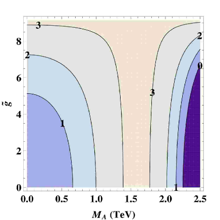
Figure 1: Contour plot for $a$ in the $(M_{A},\tilde{g})$ plane, for $S=0.3$ in NMWT ($d({\rm R})=6$). We plot contours for $a=0,1,2,3$, and $3\leq a\leq a_{\rm max}=d({\rm R})/(2\pi S)\simeq 3.18$ (central region). The running regime corresponds to the $a=0$ contour, which is on the lower right of the parameter space. Walking dynamics requires $a={\cal O}(1)>0$, which is achieved for a large portion of the parameter space.

Fig. 1 displays a contour plot of $a$ in the $(M_{A},\tilde{g})$ plane for $S=0.3$, in NMWT ($d({\rm R})=6$). This plot is obtained after imposing Eqs. (15) and (16). Notice that $a={\cal O}(1)$ for a large portion of the parameter space, since the maximum value of $a$ is found to be $a_{\rm max}=d({\rm R})/(2\pi S)$, and this gives 3.18 for $S=0.3$ and $d({\rm R})=6$. The running regime, $a=0$, is only attained for large values of $M_{A}$. However walking regimes, $a={\cal O}(1)$, are also compatible with smaller values of $M_{A}$. For example, if we require $1<a<2$ with $S=0.3$ in NMWT, from Fig (1) we see that this is both possible for $M_{A}\gtrsim$ 2.0 TeV and $M_{A}\lesssim$ 1.0 TeV. Although a walking regime with large values of $M_{A}$ is more plausible, since this is more naturally achieved by moving away from a running regime, a walking scenario with small values of $M_{A}$ cannot be excluded based solely on the WSRs analysis.

II.2 Electroweak Parameters

If the $\kappa$ parameter of Eq. (14) is negligibly small, then the fermion Lagrangian of Eq. (6) describes a “universal” theory, in the sense that all the corrections to the electroweak observables show up in gauge current correlators. If this is the case the new physics effect on the low-energy observables are fully accounted for by the Barbieri et. al. parameters Barbieri:2004qk . In our model these are

$$\hat{S} = \frac{g^{2}(1-\chi^{2})}{2\tilde{g}^{2}+g^{2}(1+\chi^{2})}\ ,$$

$$\hat{T} = 0\ ,$$

$$W = M_{W}^{2}\frac{g^{2}\left(M_{A}^{2}+M_{V}^{2}\ \chi^{2}\right)}{\left(2\tilde{g}^{2}+g^{2}(1+\chi^{2})\right)M_{A}^{2}M_{V}^{2}}\ ,$$

$$Y = M_{W}^{2}\frac{{g^{\prime}}^{2}\left(M_{A}^{2}+M_{V}^{2}\ \chi^{2}\right)}{\left(2\tilde{g}^{2}+{g^{\prime}}^{2}(1+\chi^{2})\right)M_{A}^{2}M_{V}^{2}}\ ,$$

$$\hat{U} = 0\ ,$$

$$V = 0\ ,$$

$$X = gg^{\prime}\frac{M_{W}^{2}}{M_{A}^{2}M_{V}^{2}}\frac{M_{A}^{2}-M_{V}^{2}\ \chi^{2}}{\sqrt{\left(2\tilde{g}^{2}+g^{2}(1+\chi^{2})\right)\left(2\tilde{g}^{2}+{g^{\prime}}^{2}(1+\chi^{2})\right)}}\ .$$ (23)

It is important to notice that these are the electroweak parameters from the pure technicolor sector only. Important negative contributions to $\hat{S}$ (or $S$) and positive contributions to $\hat{T}$ (or $T$) can arise from a mass splitting between the techniup and the technidown fermions (which can arise from the ETC sector) or from new nondegenerate lepton doublets, with either Majorana or Dirac neutrinos. A new lepton doublet is actually required in MWT, where it is introduced to cure the SU(2) Witten anomaly, and suffices to bring $S$ and $T$ to within 1$\sigma$ of the experimental expectation value Foadi:2007ue . Without these extra contributions, if the underlying gauge theory is NMWT (with three colors in the two-index symmetric representation), the naive one-loop contribution to $S$ is $S=1/\pi\simeq 0.3$. Taking this as the true value of $S$, the prediction for $\hat{S}$ is almost everywhere in the parameter space within 2$\sigma$ for a light Higgs and 3$\sigma$ for a heavy Higgs. If NMWT is very close to the conformal window $S$ can even be smaller: this scenario was considered in Ref. Foadi:2007se , where $\hat{S}$ was taken as a viable input (within 1$\sigma$), and the other electroweak parameters, like $Y$ and $W$, were shown to impose lower bounds on $M_{A}$ and $\tilde{g}$.

II.3 Parameter Space of NMWT

In our analysis we will take zero $\kappa$, since it affects the tree-level anomalous couplings highly constrained by experiments. We take $S=0.3$ corresponding to its naive value in NMWT.

The remaining parameters are $M_{A},\ \tilde{g},\ s$ and $M_{H}$, with $s$ and $M_{H}$ having a sizable effect in processes involving the composite Higgs .

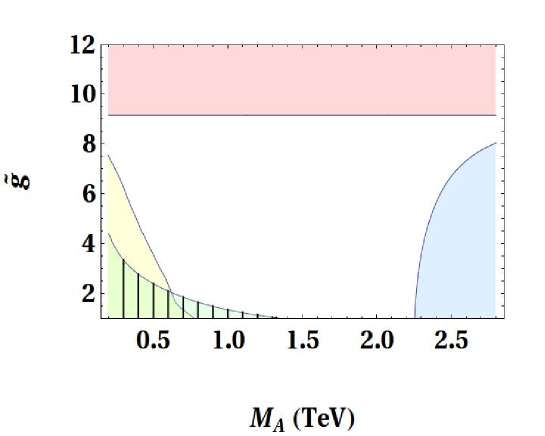
Figure 2: Bounds, for $S=0.3$, in the $(M_{A},\tilde{g})$ plane from: (i) CDF direct searches of $R_{1}^{0}$ at Tevatron, in $p\bar{p}\rightarrow e^{+}e^{-}$, for $s=1$ and $M_{H}=200$ GeV. The forbidden regions is the uniformly shaded one in the left corner. The parameters $M_{H}$ and $s$ affect indirectly the Tevatron bounds by changing the BR of the $Z$ boson decay to two composite Higgsses. However, we have checked that the effects on the constraints coming from varying the parameter $s$ and $M_{H}$ are small. (ii) Measurement of the electroweak parameters W and Y at 95% confidence level. The forbidden region is the striped one in the left corner. (iii) The constraint $a>0$, where $a$ is defined in Eq. (22). The corresponding limiting curve is given by Eq. (25). The forbidden region is the shaded one in the right corner. (iv) Consistency of the theory: no imaginary numbers for physical quantities like $F_{V}$ and $F_{A}$ . The forbidden region is the horizontal stripe in the upper part of the figure. The limiting curve here is given by Eq. (24). We repeat that the shaded regions are excluded.

CDF imposes lower bounds on $M_{A}$ and $\tilde{g}$ from direct searches of $R_{1}^{0}$ in the $p\bar{p}\rightarrow e^{+}e^{-}$ process, as shown by the uniformly shaded region in the lower left of Fig 2. To present this bound we have applied the CDF public results of Ref. CDF-limit to our model. Additional lower bounds on $M_{A}$ and $\tilde{g}$ come from the electroweak parameters $W$ and $Y$, as explained in Ref. Foadi:2007se . The measurements of $W$ and $Y$ exclude the striped region on the lower left in Fig 2 at 95% confidence level (which corresponds roughly to the $2\sigma$ limit of a one-dimensional distribution).

The upper bound for $\tilde{g}$,

$$\tilde{g}<\sqrt{\frac{8\pi}{S}}\ ,$$ (24)

is dictated by the internal consistency of the model. For $S=0.3$ this gives $\tilde{g}\lesssim 9.15$, and is shown by the upper horizontal line in Fig 2. The upper bound for $M_{A}$ corresponds to the value for which both WSR’s are satisfied in a running regime, and above which $a$ in Eq. (22) becomes negative:

$$M_{A}^{2}<\frac{4\pi F_{\pi}^{2}}{S}\left(1+\frac{1}{\sqrt{1-\frac{\tilde{g}^{2}S}{8\pi}}}\right)\ .$$ (25)

This is shown by the lower right curve in Fig 2.

III Phenomenology

We use the CalcHEP package Pukhov:2004ca since it is a convenient tool to investigate collider phenomenology. The LanHEP package Semenov:2008jy has been used to derive the Feynman rules for the model.

We tested the CalcHEP model implementation in different ways. We have implemented the model in both unitary and t’Hooft-Feynman gauge, and checked the gauge invariance of the physical output. We investigated the Custodial Technicolor (CT) limit Foadi:2007se of the model, corresponding to $r_{2}=r_{3}=0$, for which $S=0$ and $M_{A}=M_{V}$. If we further require $s=0$ this model is then identical to the degenerate BESS model (D-BESS) Casalbuoni:1995qt for which results are available in the literature Casalbuoni:2000gn . We find agreement with the latter for the widths and BR’s.

New physics signals are expected from the vector meson and the composite Higgs sectors. Here we focus on the production at LHC of the vector mesons through DY and VBF channels, as well as the production of the composite Higgs in association with a weak gauge boson. We compare our results with the ones for Higgsless models Birkedal:2005yg ; He:2007ge and on the associate Higgs production with the analysis done by Zerwekh Zerwekh:2005wh .

III.1 Heavy Vectors: Masses, Decay Widths and Branching Ratios

One important consequence of the failure of the second WSR Appelquist:1998xf ; Foadi:2007ue is the possible mass spectrum inversion of the vector and axial spin one mesons.

Figure 3: Mass splittings $M_{V}-M_{A}$ (left) and $M_{R_{2}^{\pm}}-M_{R_{1}^{\pm}}$ (right). The dotted lines are for $\tilde{g}=5$ while the solid lines are for $\tilde{g}=2$.

In Fig. 3 (left) we plot $M_{V}-M_{A}$ as a function of $M_{A}$ for two reference values of $\tilde{g}$ and $S=0.3$. For generic values of $S$ the inversion occurs for

$${M}^{\rm inv}=\sqrt{\frac{4\pi}{S}}F_{\pi}\ .$$ (26)

This gives ${M}^{\rm inv}\simeq 1.6$ TeV for $S=0.3$, as clearly shown in the plot. Fig. 3 (right) shows $M_{R_{2}^{\pm}}-M_{R_{1}^{\pm}}$ as a function of $M_{R_{1}^{\pm}}$, where $R_{1}^{\pm,0}$ ($R_{2}^{\pm,0}$) are the lighter (heavier) vector resonances, with tree-level electroweak corrections included. This mass difference is always positive by definition, and the mass inversion becomes a kink in the plot. Away from ${M}^{\rm inv}$ $R_{1}$ ($R_{2}$) is an axial (vector) meson for $M_{A}<{M}^{\rm inv}$, and a vector (axial) meson for $M_{A}>{M}^{\rm inv}$. The mass difference in Fig. 3 is proportional to $\tilde{g}^{2}$, and becomes relatively small for $\tilde{g}=2$. The effects of the electroweak corrections are larger for small $\widetilde{g}$ couplings. For example, the minimum of $M_{R_{2}^{\pm}}-M_{R_{1}^{\pm}}$ is shifted from ${M}^{\rm inv}\simeq 1.59$ TeV to about 1 TeV for $\tilde{g}=2$. To help the reader we plot in Fig. 4 the actual spectrum for the vector boson masses versus $M_{A}$. Preliminary studies on the lattice of MWT and the mass inversion issue appeared in Ref. DelDebbio:2008zf .

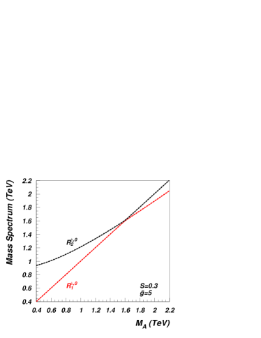
Figure 4: The mass spectrum of the $M_{R^{\pm,0}_{1,2}}$ vector mesons versus $M_{A}$ for $\tilde{g}=2$ (left) and $\tilde{g}=5$ (right). The masses of the charged vector mesons are denoted by solid lines, while the masses of the neutral mesons are denoted by dashed lines.

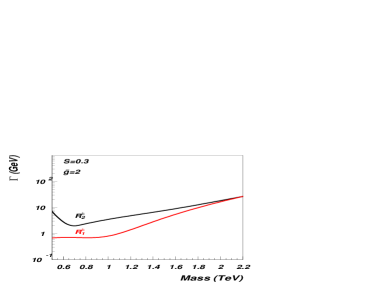
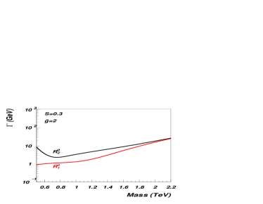
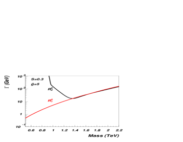
Figure 5: Decay width of the charged (first row) and neutral (second row) vector mesons for $S=0.3$ and $\tilde{g}=2,5$. We take $M_{H}=0.2\ \textrm{TeV},\ s=0$.

The widths of the heavy vectors are displayed in Fig. 5. The lighter meson, $R_{1}$, is very narrow. The heavier meson, $R_{2}$, is very narrow for small values of $\tilde{g}$. In fact in this case $M_{R_{2}}\simeq M_{R_{1}}$, forbidding decays of $R_{2}$ to $R_{1}$ (+anything). For large $\tilde{g}$, $R_{2}$ is very narrow for large masses, but then becomes broader when the $R_{2}\to R_{1},X$ channels open up, where $X$ is a SM gauge boson. It becomes very broad when the $R_{2}\to 2R_{1}$ decay channel opens up. The former are only important below the inversion point, where $R_{1}$ is not too heavy. The latter is only possible when $R_{2}$ is essentially a spin one vector and $M_{R_{2}}>2M_{R_{1}}$.

The narrowness of $R_{1}$ (and $R_{2}$, when the $R_{2}\to R_{1},X$ channels are forbidden) is essentially due to the small value of the $S$ parameter. In fact for $S=0$ the trilinear couplings of the vector mesons to two scalar fields of the strongly interacting sector vanish. This can be understood as follows: the trilinear couplings with a vector resonance contain a derivative of either the Higgs or the technipion, and this can only come from $r_{3}$ in Eq. (1). Since $r_{3}=0$ implies $S=0$, as Eqs. (20) and (19) show explicitly, it follows that the decay width of $R_{1}$ and $R_{2}$ to two scalar fields vanishes as $S\rightarrow 0$. As a consequence, for $S=0$ the vector meson decays to the longitudinal SM bosons are highly suppressed, because the latter are nothing but the eaten technipions. (The couplings to the SM bosons do not vanish exactly because of the mixing with the spin one resonances.) A known scenario in which the widths of $R_{1}$ and $R_{2}$ are highly suppressed is provided by the D-BESS model Casalbuoni:2000gn , where the spin one and the spin zero resonances do not interact. Therefore, in D-BESS all couplings involving one or more vector resonances and one or more scalar fields vanish, not just the trilinear coupling with one vector field. The former scenario requires $r_{2}=r_{3}=s=0$, the latter only requires $r_{3}=0$. A somewhat intermediate scenario is provided by CT, in which $r_{2}=r_{3}=0$ but $s\neq 0$. Narrow spin one resonances seems to be a common feature in various models of dynamical electroweak symmetry breaking. (see for example Ref. Brooijmans:2008se ). Within our effective Lagrangian (1) this property is linked to having a small $S$ parameter. If it turns out that broader spin one resonances are observed at the LHC this fact can be accounted for by including operators of mass dimension greater than four, as shown in Sec. III.5.

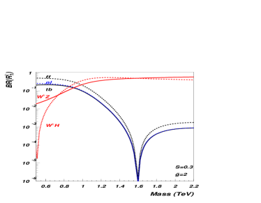
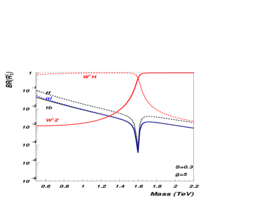
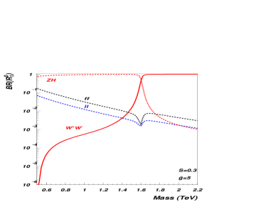
Figure 6: Branching ratios of the charged (first row) and neutral (second row) $R_{1}$ resonance for $S=0.3$ and $\tilde{g}=2,5$. We take $M_{H}=0.2\ \textrm{TeV},s=0$

The $R_{1}$ branching ratios are shown in Fig. 6. The wild variations observed in the plots around $1.6$ TeV reflects the mass inversion discussed earlier. Here the mixing between $R_{1}^{a}$ and $\widetilde{W}^{a}$, with $a=0,\pm$, vanishes, suppressing the decay to SM fermions.

The other observed structure for the decays in $ZH$ and $WH$, at low masses, is due to the opposite and competing contribution coming from the technicolor and electroweak sectors. This is technically possible since the coupling of the massive vectors to the longitudinal component of the gauge bosons and the composite Higgs is suppressed by the small value of S.

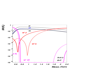
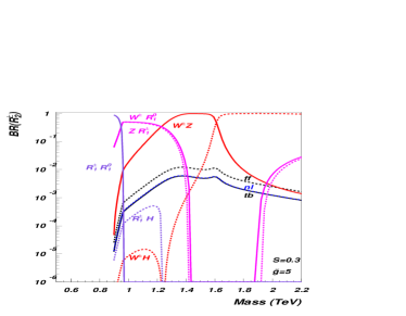
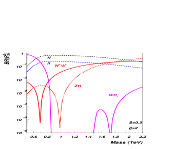
Figure 7: Branching ratios of the charged (first row) and neutral (second row) $R_{2}$ resonance for $S=0.3$ and $\tilde{g}=2,5$ . We take $M_{H}=0.2\ \textrm{TeV},s=0$

Now we consider the $R_{2}$ BR’s displayed in Fig. 7. Being $R_{2}$ heavier than $R_{1}$ by definition, new channels like $R_{2}\rightarrow 2R_{1}$ and $R_{2}\rightarrow R_{1}X$ show up, where $X$ denotes a SM boson. Notice that there is a qualitative difference in the $R_{2}$ decay modes for small and large values of $\tilde{g}$. First, for small $\tilde{g}$ the $R_{2}-R_{1}$ mass splitting is not large enough to allow the decays $R_{2}\rightarrow 2R_{1}$ and $R_{2}\rightarrow R_{1}H$, which are instead present for large $\tilde{g}$. Second, for small $\tilde{g}$ there is a wide range of masses for which the decays to $R_{1}$ and a SM vector boson are not possible, because of the small mass splitting. The BR’s to fermions do not drop at the inversion point, because the $R_{2}-\widetilde{W}$ mixing does not vanish.

III.2 Drell-Yan Production: $p,p\to R_{1,2}$

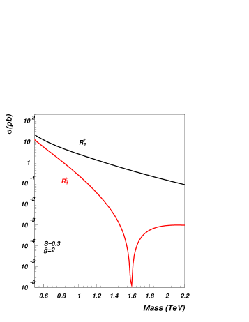
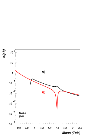
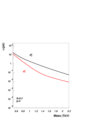
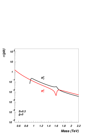
Figure 8: Drell-Yan production of the $R_{1,2}^{\pm}$ (first row) and $R_{1,2}^{0}$ (second row) resonances, with $S=0.3$ and $\tilde{g}=2,5$.

Spin one resonances can be produced at LHC through the DY processes $pp\to R_{1,2}$. The corresponding cross sections are shown in Fig. 8. Consider first the production of $R_{2}^{\pm}$, since the latter is less affected than $R_{1}^{\pm}$ by the presence of the mass inversion point. The cross section decreases as $\tilde{g}$ grows, because of the reduced $R_{2}-\widetilde{W}$ mixing. In going from $\tilde{g}=2$ to $\tilde{g}=5$ the decrease in the production cross-section of $R_{2}^{\pm}$ is roughly one or two orders of magnitude. This is expected since the leading order contribution to the coupling between $R_{2}^{\pm}$ and fermions is explicitly proportional to $\tilde{g}^{-2}$, as it is in the D-BESS model Casalbuoni:2000gn .

As explained in Sec. III.1 the $R_{1}^{\pm}$ resonance becomes fermiophobic at the inversion point, causing the corresponding DY production to drop. In our model the new vectors are fermiophobic only at the mass inversion point differentiating it from a class of Higgsless model in which the charged $W^{\prime}$ resonance is taken to have strongly suppressed couplings to the light fermions for any value of the vector masses.

To estimate the LHC reach for DY production of the $R_{1,2}^{0}$ and $R_{1,2}^{\pm}$ resonances we study the following lepton signatures:

• $\ell^{+}\ell^{-}$ signature from the process $pp\to R^{0}_{1,2}\to\ell^{+}\ell^{-}$

• $\ell+{/\!\!\!\!\!\>E}_{T}$ signature from the process $pp\to R^{\pm}_{1,2}\to\ell^{\pm}\nu$

• $3\ell+{/\!\!\!\!\!\>E}_{T}$ signature from the process $pp\to R^{\pm}_{1,2}\to ZW^{\pm}\to 3\ell\nu$ ,

where $\ell$ denotes a charged lepton – electron or muon and ${/\!\!\!\!\!\>E}_{T}$ is the missing transverse energy. We apply detector acceptance cuts of $|\eta^{\ell}|<2.5$ and $p_{T}^{\ell}>15$ GeV on the rapidity and transverse momentum of the leptons. For signature (1) we use the di-lepton invariant mass distribution $M_{\ell\ell}$ to separate the signal from the background. For signatures (2) and (3) we use instead the transverse mass variables $M^{T}_{\ell}$ and $M^{T}_{3\ell}$ bagger :

$$(M^{T}_{\ell})^{2}=[\sqrt{M^{2}(\ell)+p_{T}^{2}(\ell)}+|{/\!\!\!\!\!\>p}_{T}|]^{2}-|\vec{p}_{T}(\ell)+{/\!\!\!\!\!\>\vec{p}}_{T}|^{2}$$ (27)

$$(M^{T}_{3\ell})^{2}=[\sqrt{M^{2}(\ell\ell\ell)+p_{T}^{2}(\ell\ell\ell)}+|{/\!\!\!\!\!\>p}_{T}|]^{2}-|\vec{p}_{T}(\ell\ell\ell)+{/\!\!\!\!\!\>\vec{p}}_{T}|^{2}$$ (28)

We also add a cut on the transverse missing energy ${/\!\!\!\!\!\>E}_{T}>15$ GeV. We consider the representative parameter space points $\tilde{g}=2,5$ and $M_{A}=0.5,1,1.5,2$ TeV for our plots and discussion.

The invariant mass and transverse mass distributions for signatures (1)-(3) are shown in Figs. 9-11.

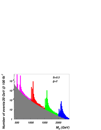
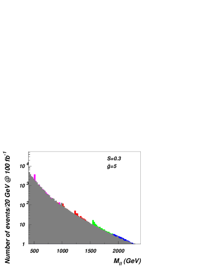
Figure 9: Dilepton invariant mass distribution $M_{\ell\ell}$ for $pp\to R^{0}_{1,2}\to\ell^{+}\ell^{-}$ signal and background processes. We consider $\tilde{g}=2,5$ respectively and masses $M_{A}=0.5$ Tev (purple), $M_{A}=1$ Tev (red), $M_{A}=1.5$ Tev (green) and $M_{A}=2$ Tev (blue).

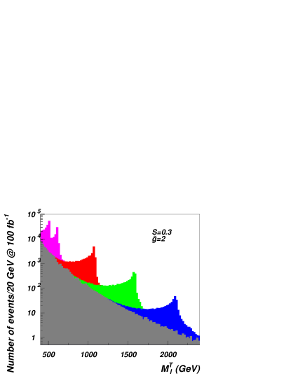
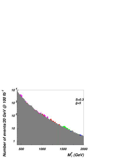
Figure 10: $M^{T}_{\ell}$ mass distribution for $pp\to R^{\pm}_{1,2}\to\ell^{\pm}\nu$ signal and background processes. We consider $\tilde{g}=2,5$ respectively and masses $M_{A}=0.5$ Tev (purple), $M_{A}=1$ Tev (red), $M_{A}=1.5$ Tev (green) and $M_{A}=2$ Tev (blue).

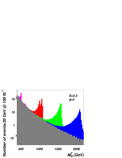
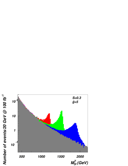
Figure 11: $M^{T}_{3\ell}$ mass distribution for $pp\to R^{\pm}_{1,2}\to ZW^{\pm}\to 3\ell\nu$ signal and background processes. We consider $\tilde{g}=2,5$ respectively and masses $M_{A}=0.5$ Tev (purple), $M_{A}=1$ Tev (red), $M_{A}=1.5$ Tev (green) and $M_{A}=2$ Tev (blue).

In the left frames of Figs. 9 and  10, corresponding to $\tilde{g}=2$, clear signals from the leptonic decays of $R^{0}_{1,2}$ and $R^{\pm}_{1,2}$ are seen even for 2 TeV resonances. Moreover Fig. 9 demonstrates that for $\tilde{g}=2$ both peaks from $R^{0}_{1}$ and $R^{0}_{2}$ may be resolved. The lepton energy resolution effects should not visibly affect the presented distributions. In the case of signature (2) a double-resonance peak is also seen at low mass, but the transverse mass distribution $M^{T}_{\ell}$ is not able to resolve the signal pattern as well as the $M^{\ell\ell}$ distribution for signature (1), because of the presence of missing transverse momenta from the neutrino. This analysis must be improved via a full-detector simulation. However, for larger masses only a single resonance is visible because the $R^{\pm}_{1}$ coupling to fermions is strongly suppressed. This is a distinguishing footprint of the NMWT model at higher masses closer to the inversion point: only a single peak from the $R_{2}^{\pm}$ will appear in the single lepton channel while a double peak should be visible in the di-lepton channel.

Let us now turn to the case of $\tilde{g}=5$ in the right frames of Figs. 9 and 10. For large $\tilde{g}$ the $Rff$ couplings are suppressed, so observing signatures (1) and (2) could be problematic (quantative results for the LHC reach for all signatures are presented below). However, for large $\tilde{g}$, the triple-vector coupling is enchanced, so one can observe a clear signal in the $M^{T}_{3\ell}$ distribution presented in Fig. 11. At low masses the decays of the heavy vector mesons to SM gauge bosons are suppressed and the signal disappears. This mass range can, however, be covered with signatures (1) and (2) as we demonstrate below.

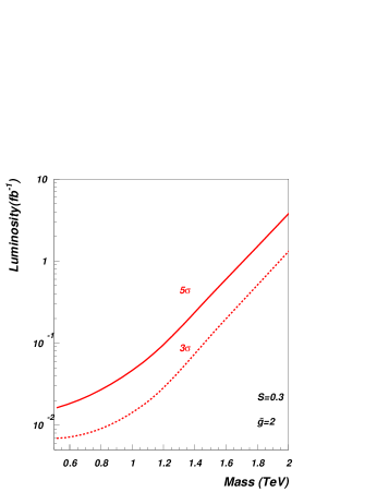
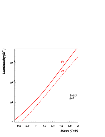
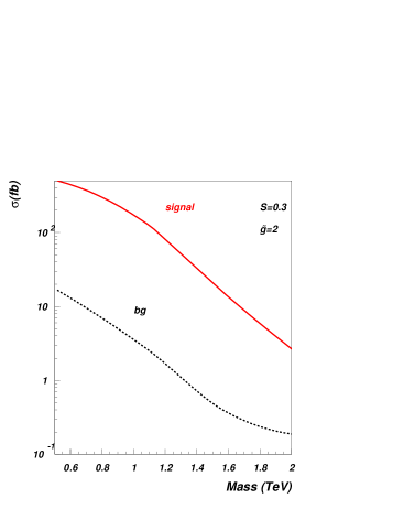
Figure 12: LHC reach for the $R^{0}_{1,2}$ resonance signal in $pp\to R^{0}_{1,2}\to e^{+}e^{-}$ with $S=0.3$ and $\tilde{g}=2,5$. Top row: the required integrated luminosisty for achieveing a 5$\sigma$ and a 3$\sigma$ significance. Bottom row: the signal and background cross sections for this process.

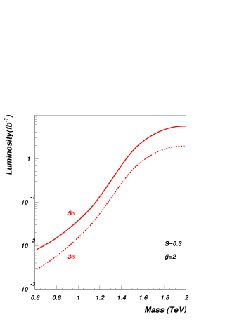
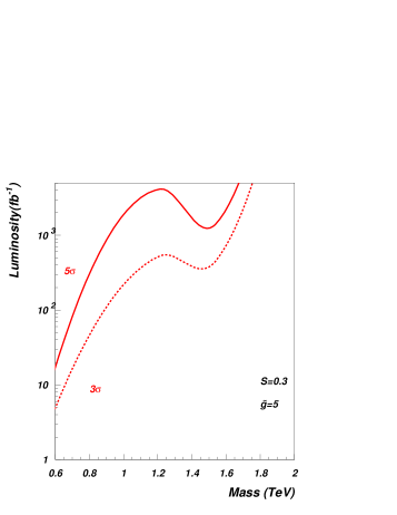
Figure 13: LHC reach for the $R^{\pm}_{1,2}$ resonance signal in $pp\to R^{\pm}_{1,2}\to\ell{/\!\!\!\!\!\>E}_{T}$ signature with $S=0.3$ and $\tilde{g}=2,5$. Top row: the required integrated luminosisty for achieveing a 5$\sigma$ and a 3$\sigma$ significance. Bottom row: the signal and background cross sections for this process.

We end this section by quantifying the LHC reach for signatures (1)-(3) in terms of the luminosity required to observe the $R_{1,2}$ mass peaks at a significance of 3 and 5 sigma. To do so we define the signal as the difference between the NMWT cross section and the SM cross section in a certain mass window around the peak. We optimize the invariant or transverse mass window cuts, on a case by case basis, for each signature and parameter space point. For example, signatures (2) and (3) require assymetric mass window cuts since the transverse one- and tri-lepton mass distribution have low-end tails. We single out the most significant peak when applying the mass window cut. The significance of the signal is then defined as the number of signal events divided by the square root of the number of background events when the number of events is large, while a Poisson distribution is used when the number of events is small.

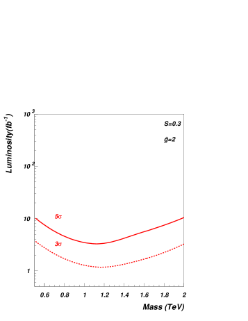
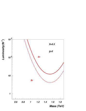
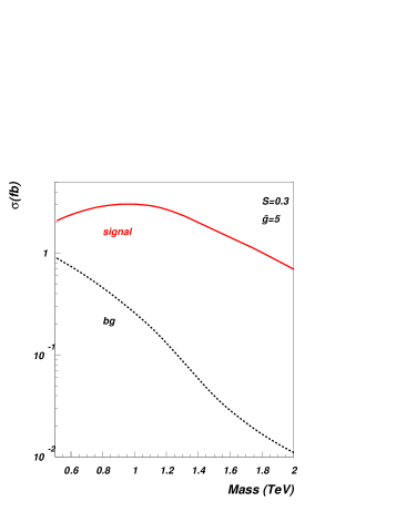
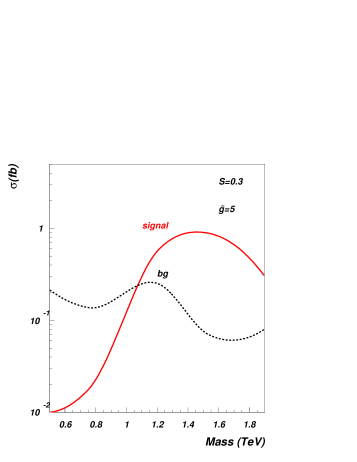
Figure 14: LHC reach for the $R^{\pm}_{1,2}$ resonance signal in $pp\to R^{\pm}_{1,2}\to W^{\pm}Z\to 3\ell{/\!\!\!\!\!\>E}_{T}$ signature with $S=0.3$ and $\tilde{g}=2,5$. Top row: the required integrated luminosisty for achieveing a 5$\sigma$ and a 3$\sigma$ significance. Bottom row: the signal and background cross sections for this process.

The luminosity required for 5$\sigma$ and 3$\sigma$ significance for signature (1) is shown in the first row of plots in Fig. 12 as a function of the mass of the resonance while the signal and background cross sections are shown in the second row of plots. For $\tilde{g}=2$ one can see that even for 5 fb^-1 of integrated luminosity LHC will observe vector mesons up to 2 TeV mass through signature (1). On the other hand, for $\tilde{g}=5$ even with 100 fb^-1 integrated luminosity one would not be able to observe vector mesons heavier than 1.4 TeV in this channel. The reach of the LHC for signature (2) is quite similar to the one for signature (1) for $\tilde{g}=2$ but less promising for $\tilde{g}=5$ as one can see in Fig. 13.

The LHC reach for signature (3) is presented in Fig. 14. For $\tilde{g}=2$ the LHC will cover the whole mass range under study with 10 fb^-1 of integrated luminosity through signature (3). For $\tilde{g}=5$ it will be able to cover the large mass region inaccessible to signatures (1) and (2) through signature (3) with an integrated luminosity of 10-50 fb^-1 while the low mass region could be covered by signatures (1) and (2) with an integrated luminosity of 10-100 fb^-1. Thus signature (3) is, in a very important way, complementary to signatures (1) and (2).

III.3 Vector Boson Fusion production: $p,p\to R_{1,2},j,j$

VBF is potentially an important channel for vector meson production, especially in theories in which the vector resonances are quasi fermiophobic.

We consider VBF production of the charged $R_{1}$ and $R_{2}$ vectors. We impose the following kinematical cuts on the jet transverse momentum $p^{j}_{T}$, energy $E^{j}$, and rapidity gap $\Delta\eta^{jj}$, as well as rapidity acceptance $|\eta^{j}|$ He:2007ge ; Birkedal:2005yg :

$$|\eta^{j}|<4.5\ ,\quad p^{j}_{T}>30\mbox{ GeV}\ ,\quad E^{j}>300\mbox{ GeV}\ ,\quad\Delta\eta^{jj}>4\ .$$ (29)

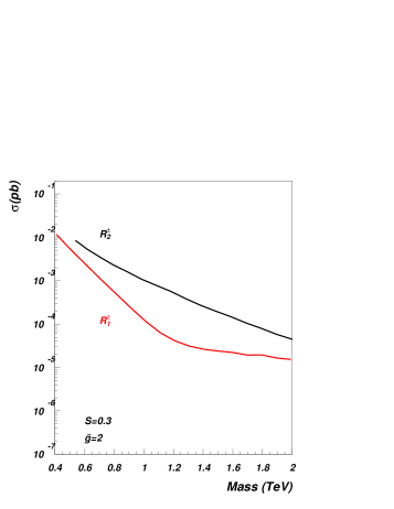
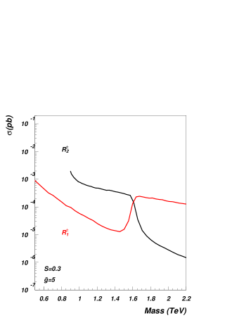
Figure 15: Vector boson fusion production cross sections for the $R_{1,2}^{\pm}$ resonances, with $S=0.3$ and $\tilde{g}=2,5$. The jet cuts are: $|\eta^{j}|<4.5$, $p^{j}_{T}>30$ GeV, $E^{j}>300$ GeV, $\Delta\eta^{jj}>4$. See text for details.

The VBF production cross section for the charged $R_{1}$ and $R_{2}$ vector resonances is shown in Fig. 15 for the set of cuts given by Eq. 29. An interesting feature of the VBF production is the observed crossover around the mass degeneracy point for $\widetilde{g}=5$. This is a direct consequence of the fact that the $R_{1,2}$ resonances switch their vector/axial nature at the inversion point. For smal $\tilde{g}$ the crossover does not occur due to the interplay between the electroweak and the Technicolor corrections. In D-BESS VBF processes are not very relevant, since there are no direct interactions between the heavy mesons and the SM vectors. However in fermiophobic Higgsless models VBF is the main production channel of the heavy resonances. Since the production rate of $R^{\pm}_{1,2}$ is below 1 fb VBF is not a promising channel at the LHC.

III.4 Composite Higgs Phenomenology

The composite Higgs phenomenology is interesting due to its interactions with the new massive vector bosons and their mixing with SM gauge bosons. We first analyze the Higgs coupling to the $W$- and $Z$- gauge bosons. In Fig. 16 (left) we present the $g_{HWW}/g_{HWW}^{SM}$ ratio as a function of $M_{A}$. The behaviour of the $g_{HZZ}$ and $g_{HWW}$ couplings are identical. We keep fixed $S=0.3$ and consider two values of $\tilde{g}$, 2 (solid line) and 5 (dashed line). We repeat the plots for three choices of the $s$ parameter $(+1,0,-1)$ depicted in black, blue and green colors respectively. The deviation of $g_{HWW}$ from $g_{HWW}^{SM}$ increases with $M_{A}$ due to the fact that we hold the $S$ parameter fixed.

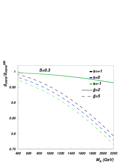
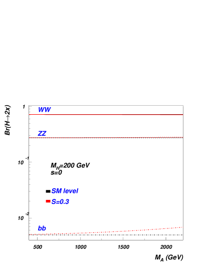
Figure 16: Left: $g_{HWW}/g_{HWW}^{SM}$ ratio as a function of $M_{A}$. The behavior of the $g_{HZZ}$ coupling is identical to the $g_{HWW}$ one. Results are presented for $S=0.3$, $\tilde{g}$=2 and 5 (solid and dashed lines respectively), and for $s=(+1,0,-1)$ (black, blue and green colors respectively).
Right: branching ratios of the composite Higgs (red) and SM Higgs (black) as function $M_{A}$ with $s=0$. $M_{H}$= 200 GeV.

One reaches deviations from the SM couplings of 20$\%$ when $M_{A}\simeq 2$ TeV. This is reflected in the small deviations of the Higgs branching ratios when compared with the SM ones as shown in Fig. 16 (right). Here we used as reference point $s=0$.

The presence of the heavy vectors is prominent in the associate production of the composite Higgs with SM vector bosons, as first pointed out in Zerwekh:2005wh . Parton level Feynman diagrams for the $pp\to WH$ and $pp\to ZH$ processes are shown in Fig. 17 (left) and Fig. 17 (right) respectively.

Figure 17: Feynman diagrams for the composite Higgs production in association with SM gauge bosons.

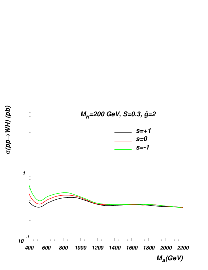
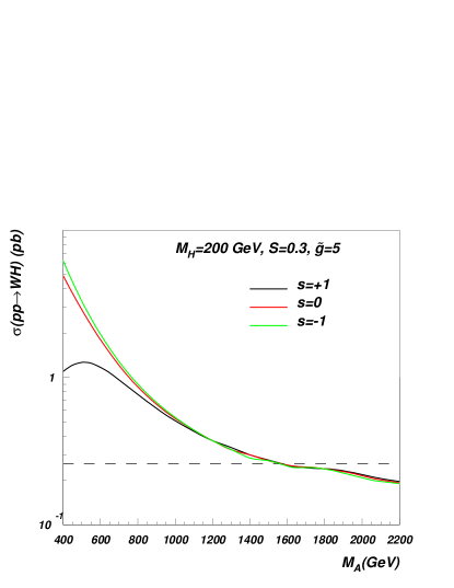
Figure 18: The cross section for $pp\to WH$ production ($W^{+}H$ and $W^{-}H$ modes are summed up) versus $M_{A}$ for $S=0.3$, $s=(+1,0,1)$ and $\tilde{g}=2$ (left) and $\tilde{g}=5$ (right). The dashed line at the bottom indicates the SM cross section level.

The resonant production of heavy vectors can enhance $HW$ and $ZH$ production by a factor 10 as one can see in Fig. 18 (right). This enhancement occurs for low values of the vector meson mass and large values of $\tilde{g}$. This behavior is shown in Fig. 18 (right) for $\tilde{g}=5$. These are values of the parameters not excluded by Tevatron data (see Fig. 2).

The contribution from heavy vector to $pp\to VH$ ($V=W^{\pm},Z$ can be clearly identified from the peaks in the invariant mass distributions of $WZZ$ or $ZZZ$ presented in Fig. 19.

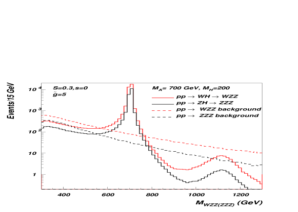
Figure 19: Invariant mass distributions of $WZZ$ or $ZZZ$ for signal (solid lines) and background (dashed lines) for 100 fb^-1.

One should consider these distributions as qualitative ones, since at the experimental level $WZZ$ or $ZZZ$ invariant masses will be reconstructed from leptons and jets in the final state with appropriate acceptance cuts applied. However, one can eventually expect that visibility of the signal will remain. Taking into account leptonic branching ratios of the two $Z$-bosons and the hadronic branching ratios for the third gauge boson (W or Z) we estimate about 40 clean events under the peak with negligible background. The second broader vector peak will not be observed.

Figure 20: Composite Higgs production cross section via the VBF mechanism.

We have also analyzed the composite Higgs production in vector boson fusion processes $pp\to Hjj$. We find that it is not enhanced with respect to the corresponding process in the SM as it is clear from Fig. 20. The behavior of the $\sigma(pp\to Hjj)$ as function of $M_{A}$ traces the one of the Higgs-gauge bosons coupling shown in Fig. 16.

III.5 Extending the Parameter Space

In Sec. III.1 we saw that the vector resonances are very narrow. The only exception occurs for the $R_{2}$ meson, when the $R_{2}\to R_{1},X$ and $R_{2}\to 2R_{1}$ channels are important ($X$ denotes a SM gauge boson). The origin of this can be attributed to the fact that in writing Eq. (1) we used only renormalizable operators. Consider for example the operator Kaymakcalan:1984bz ; Sannino:2008ha :

$$-\frac{2\gamma}{v^{2}}{\rm Tr}\left[F_{{\rm L}\mu\nu}MF_{\rm L}^{\mu\nu}M^{\dagger}\right]\ .$$ (30)

This operator was introduced many years ago by Kaymakcalan and Schechter in Kaymakcalan:1984bz and appeared for the first time in DEWSB effective Lagrangians in Sannino:2008ha . The effects of a similar Lagrangian term has been also recently discussed, in the context of four-site Higgsless model, by Chivukula and Simmons Chivukula:2008gz . This term affects several couplings. For example the $g_{V\pi\pi}$ coupling reads

$$g_{V\pi\pi}=\frac{F_{V}M_{V}}{2F_{\pi}^{2}}\left[1-\frac{1+\gamma}{1-\gamma}\frac{F_{A}^{2}}{M_{A}^{2}}\frac{M_{V}^{2}}{F_{V}^{2}}\right]\ .$$ (31)

Taking either the $M_{A}\to\infty$ or the $\gamma\to-1$ limit returns the known formula for $g_{\rho\pi\pi}$ in QCD. To better appreciate the physical content of this term we combine Eq. (30) and Eq. (1) yielding the following kinetic terms for the vector and axial states:

$$-\frac{1+\gamma}{4}(\partial_{\mu}V_{\nu}-\partial_{\nu}V_{\mu})^{2}-\frac{1-\gamma}{4}(\partial_{\mu}A_{\nu}-\partial_{\nu}A_{\mu})^{2}$$ (32)

From this it follows that requiring the vector mesons to be non-tachyonic propagating fields implies $-1<\gamma<1$. Moreover it is unreasonable to take $\gamma$ too close to either $-1$ or $1$, because this would naturally lead to infinitely large masses for the vector mesons.

Taking a value of $\gamma$ not close to $\pm 1$ but different from zero has anyway a large impact on the meson widths. In Fig. 21 the $R_{1}$ and $R_{2}$ widths are shown for both $\gamma=0$ (solid lines) and $\gamma=-0.5$ (dashed lines). The widths can increase by two orders of magnitude.

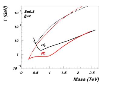
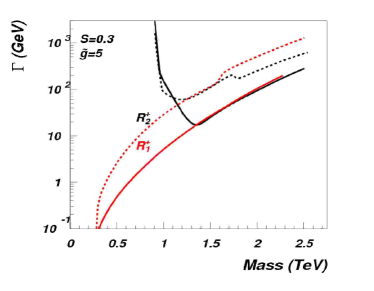
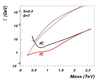
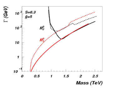
Figure 21: Decay width of the charged (first row) and neutral (second row) vector mesons for $S=0.3$ and $\tilde{g}=2,5$. The solid lines correspond to $\gamma=0$, the dashed lines correspond to $\gamma=-0.5$. We take $M_{H}=0.2\ \textrm{TeV},\ s=0$.

The DY production of the heavy vectors is unaffected by $\gamma$, at the tree level, since the fermion couplings to the vector mesons do not depend on it. We have also checked that the contributions from this term do not substantially affect the other results.

IV Conclusions

We have analyzed the potential of the Large Hadron Collider (LHC) to observe signatures of phenomenologically viable Walking Technicolor models. We studied and compared the Drell-Yan (DY) and Vector Boson Fusion (VBF) mechanisms for the production of composite heavy vectors. The DY production mechanism constitutes the most promising way to detect and study the technicolor spin one states.

We have compared, when possible, with earlier analysis and shown that our description reproduces all of the earlier results while extending them by incorporating basic properties of walking dynamics such as the mass relation between the vector and axial spin one resonances.

LHC can be sensitive to spin one states as heavy as 2 TeV. One TeV spin one states can be observed already with 100 pb^-1 integrated luminosity in the di-lepton channel. The VBF production of heavy mesons is, however, suppressed and will not be observed. The enhancement of the composite Higgs production is another promising signature.

We identified distinct DY signatures which allow to cover at the LHC, in a complementary way, a great deal of the model’s parameter space.