Boundary field induced first-order transition in the 2D Ising model: numerical study
Abstract
In a recent paper, Clusel and Fortin [J. Phys. A.: Math. Gen. 39 (2006) 995] presented an analytical study of a first-order transition induced by an inhomogeneous boundary magnetic field in the two-dimensional Ising model. They identified the transition that separates the regime where the interface is localized near the boundary from the one where it is propagating inside the bulk. Inspired by these results, we measured the interface tension by using multimagnetic simulations combined with parallel tempering to determine the phase transition and the location of the interface. Our results are in very good agreement with the theoretical predictions. Furthermore, we studied the spin-spin correlation function for which no analytical results are available.
1 Introduction
Wetting transitions are phase transitions in the surface layer of bulk systems which are induced by symmetry-breaking surface fields [1, 2]. The Ising model with a boundary magnetic field is a simple model for such a wetting problem, because Ising ferromagnets have the same critical behaviour as the analogous case of gas-fluid transitions, as has been pointed out by Nakanishi and Fisher [3]. The use of the Ising model with short range interactions for wetting studies has not only the advantage that one can use all the advanced simulation techniques which have been developed in the past years. Especially in two dimensions (2D), there are also a lot of theoretical results available for comparison.
The Ising model with a uniform boundary magnetic field on one side of a square lattice has been completely solved by McCoy and Wu [4], whereas the Ising model with a uniform bulk field can only be solved at the critical temperature [5]. For situations with fixed boundary spins or equivalently infinite boundary magnetic fields [6], or finite boundary magnetic fields [7] some exact results have also been found. In a recent paper, Clusel and Fortin [8] presented an alternative method to that developed by McCoy and Wu for obtaining some exact results for the 2D Ising model with a general boundary magnetic field and for finite-size systems. Their method is based on the fermion representation of the Ising model using a Grassmann algebra. They applied this method to study the first-order transition induced by an inhomogeneous boundary magnetic field in the 2D Ising model [9]. To be more precise, the boundary magnetic field acts on the column of spins, being positive in the lower and negative in the upper halve. By taking the thermodynamic limit exactly for a given geometry of the lattice, they obtained a simple equation for the transition line and also a threshold for the aspect ratio , where this line moves into the complex plane. This vanishing of the transition line indicates the crossover from 1D behaviour for to 2D behaviour at large , which is reflected in the behaviour of the boundary spin-spin correlation function.
The aim of this work is to check some of the predictions by carrying out Monte Carlo simulations of this model and to extend the results to parameter ranges and for observables where analytic solutions cannot be obtained. The rest of the paper is organized as follows. In Section 2 we give the definition of the model and briefly summarize the theoretical predictions. A description of the employed simulation techniques and the results of our Monte Carlo simulations are presented in Section 3, and concluding remarks can be found in Section 4.
2 Model and Theoretical Predictions
We consider a 2D Ising model with a non-homogeneous magnetic field located on one boundary of the system. The Hamiltonian is given by
| (1) |
with free boundaries in the -direction and periodic boundary conditions in the -direction. To compare our results with the theoretical predictions of Clusel and Fortin [9], we consider the same profile of the boundary magnetic field acting on the column of spins: for and for , with .

In the limit of zero temperature, by using simple energetic arguments, Clusel and Fortin [9] showed that for small all spins are aligned in one direction as in the bulk case for , see also Figure 1. With increasing , however, depending on the aspect ratio two different interfaces can be formed. If the interface is localized near the boundary, whereas for the interface is propagating inside the bulk. The critical ratio marks the crossover from a 1D behaviour for towards a 2D behaviour at large . For and non-zero temperatures , with the abbreviations and , the equation for the first-order transition line in the -plane turns out to be a quadratic equation in [9]:
| (2) | |||
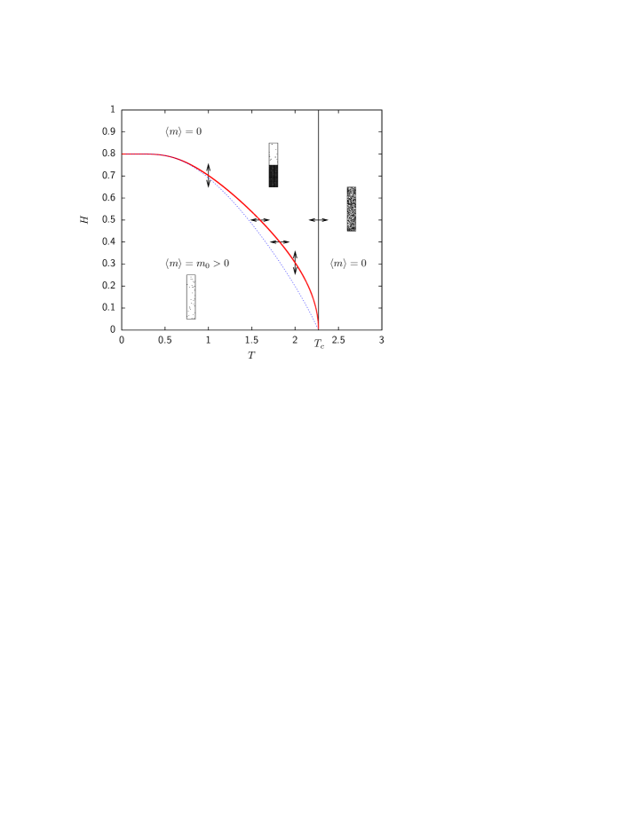
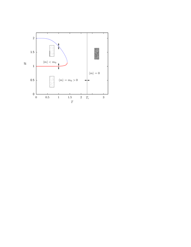
In Figure 2 we show the phase diagram for a system with aspect ratio (and ). In the low-temperature regime we can approximate the above expression by comparing the energy of the interface with the energy induced by the magnetic field. This leads to , where and are the known interface tension and the spontaneous magnetization of the pure 2D Ising model, respectively. This approximation reproduces the exact low- expansion, , and works very well for as one can see in Figure 2 (thin dashed line). Since vanishes much faster than as , also this point is reproduced exactly, but the slope of the approximate transition line at does not diverge as for the exact solution.
Due to the first-order transition induced by the inhomogeneous boundary magnetic field, the second-order phase transitions across the vertical line at are transitions from a region where an interface in the bulk separates two ordered domains of opposite magnetization from a disordered regime above the transition temperature. Therefore, the system undergoes a transition without a change in the magnetization which is zero in both phases, cf. Figure 2, but the width of the magnetization distribution does change.
3 Numerical Results
Since we are primarily interested in the location of the interface induced by the boundary field, we first performed simulations at low temperatures to generate a well-defined interface. To overcome the slow dynamics at low temperatures we developed a combination of the multimagnetic algorithm with the parallel tempering method [10] for which we used two different schemes: In the first scheme, we kept the magnetic field value fixed and simulated replica of the system at different temperatures . In the second scheme, we kept the temperature fixed and used different values of the magnetic field .
To construct the weight function for the multimagnetic part of the algorithm, we employed an accumulative recursion, described in detail in Refs. [10] and [11]. Statistical averages were taken over runs of Monte Carlo (MC) steps, where one MC step consists of one full multimagnetical lattice sweeps for all 32 replica and one attempted parallel tempering exchange of all adjacent replica. With this method we were able to study systems with to spins for aspect ratios , and , for further details see Table 1.
| method | measurements | ||||
|---|---|---|---|---|---|
| 0.2 | 0.4 | 1.6 – 2.2 | 80 – 2000 | PT | |
| 0.2 | 0.5 | 1.4 – 1.9 | 80 – 2000 | PT | |
| 0.2 | 0.5 | 2.1 – 2.3 | 80 – 180500 | SC | – |
| 0.2 | 0.7 – 0.9 | 1.0 | 80 – 640 | PT | |
| 0.2 | 0.285 – 0.316 | 2.0 | 80 – 2000 | PT | |
| 0.25 | 0.4 | 1.9 – 2.1 | 256 – 2500 | PT | |
| 0.25 | 0.5 | 1.5 – 1.9 | 64 – 2000 | PT | |
| 0.25 | 0.5 | 2.0 – 2.3 | 64 – 6400 | SC | – |
| 0.25 | 0.7 – 0.8 | 1.5 | 64 – 1600 | PT | |
| 0.5 | 0.5 | 2.2 – 2.35 | 50 – 3200 | PT | |
| 0.5 | 0.9 – 1.1 | 1.0 | 50 – 5000 | PT | |
| 0.5 | 1.5 – 2.0 | 1.0 | 50 – 3872 | PT |
Let us first discuss the data obtained for the case . For this value of the aspect ratio, the phase diagram as predicted by Clusel and Fortin [9] is shown in Figure 2. The thick line indicates the first-order transitions from the fully magnetized state with to the mixed state with an interface extending across the bulk. To check the nature of these transitions we measured the probability density of the magnetization at four points along the transition line. In the first two cases, we kept the boundary magnetic field constant ( and ) and varied the temperature to locate the transition point, and in the other two cases, we fixed the temperature ( and ) and varied the boundary magnetic field. These points are indicated by the double-headed arrows in Figure 2.
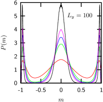
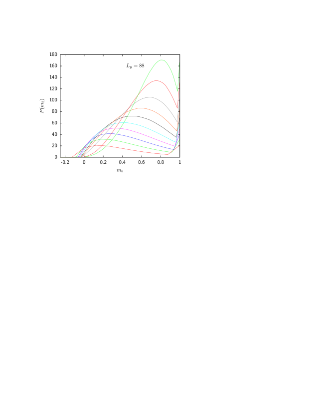
In the following we illustrate our procedure for obtaining the first-order transition point and the associated interface tension for the case of fixed . A level plot of the magnetization density as a function of temperature is shown in Figure 3 (left). For each lattice size, a pseudo-transition point can be defined by varying the temperature until the peaks at and are of equal height, which can be achieved by histogram reweighting. The interface tension can then be estimated from [12]
| (3) |
where is the value of the peaks and denotes the minimum in between, see Figure 3 (right). The length of the interface is denoted by , which is in the case of .
The thus defined pseudo-transition temperatures approach the infinite-volume transition temperature as , and for the final estimate of , we performed a fit according to
| (4) |
At fixed one proceeds analogously by varying the magnetic field , i.e., the roles of and are just interchanged. For all four cuts at constant surface field or temperature we find a good agreement with the infinite-volume transition points derived from Equation (2) and a clearly nonzero interface tension, see Table 2.
| (exact) | ||||
|---|---|---|---|---|
| 0.2 | 0.4 | 1.84(1) | 1.82252 | 0.18(1) |
| 0.2 | 0.5 | 1.60(1) | 1.59497 | 0.32(2) |
| 0.25 | 0.5 | 1.91(1) | 1.95845 | 0.09(1) |
| (exact) | ||||
| 0.2 | 1.0 | 0.72(1) | 0.702352 | 0.82(2) |
| 0.2 | 2.0 | 0.305(3) | 0.305928 | 0.12(1) |
| 0.25 | 1.5 | 0.73(1) | 0.762807 | 0.24(1) |
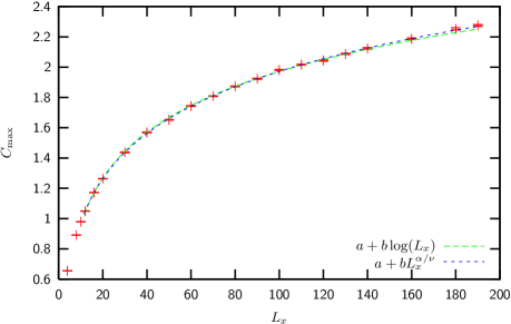
We also checked the critical behaviour along the line of second-order transitions at . To this end we run at single-cluster simulations (suitably adapted to the surface field) for systems with to spins and performed a finite-size scaling (FSS) analysis to determine the transition point and some critical exponents. This particular value of the magnetic field has been chosen because of the relatively large temperature gap between the boundary field induced first-order transition and the bulk phase transition. Between each measurement we performed one sweep, which here consists of single-cluster updates with chosen such that , where is the average cluster size. For every run we generated sweeps, and recorded the time series of the energy density and the magnetization density. Using these time series, we can compute the specific heat, , the (finite lattice) susceptibility, , and the Binder cumulant in the vicinity of the simulation point by reweighting.
In this way we can use the maxima of the (finite lattice) susceptibility to detect the pseudo-critical points and can obtain an estimate for from a linear least-square fit of their scaling behaviour, , assuming thus the exact value according to the universality class of the 2D Ising model. This leads to an estimate for the critical temperature, , which is in very good agreement with the exact value. The FSS ansatz for the (finite lattice) susceptibility maxima is taken as usual as . From a (linear) least-square fit, we find that is in perfect agreement with the exact value . Concerning the specific heat we expect in the case of the Onsager exponent a logarithmic divergence of the form . Indeed, the data can be fitted nicely with this ansatz, cf. Figure 4. We also tried an unbiased fit using the power-law ansatz , which gives us , verifying the expected value.
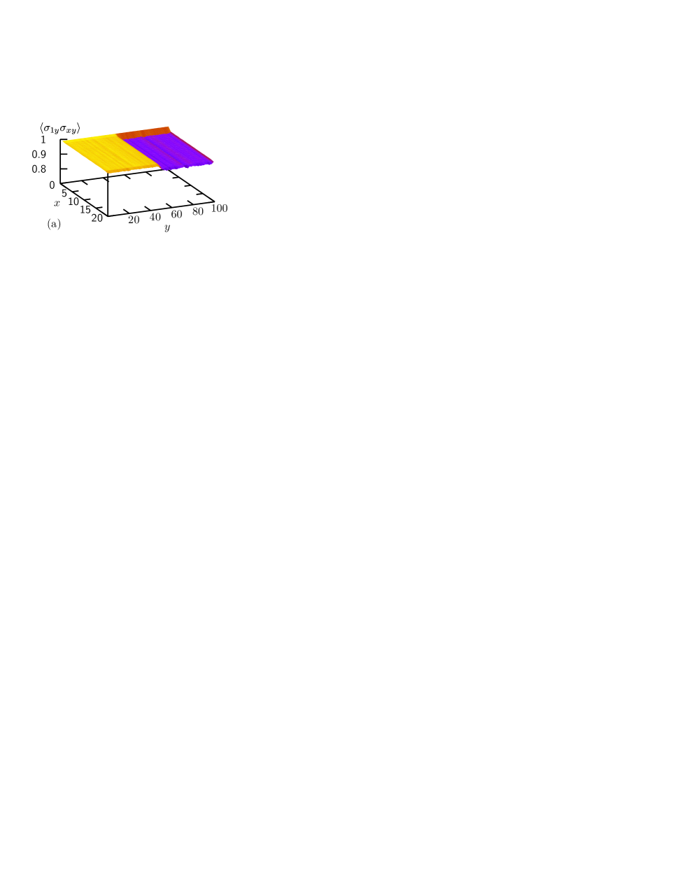
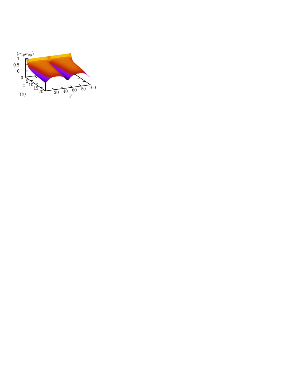
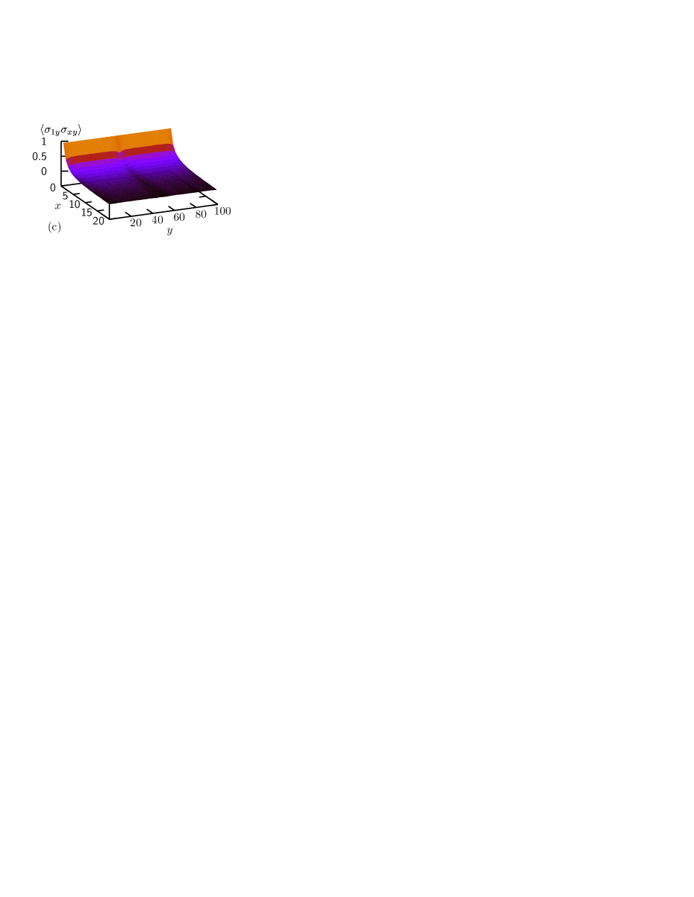
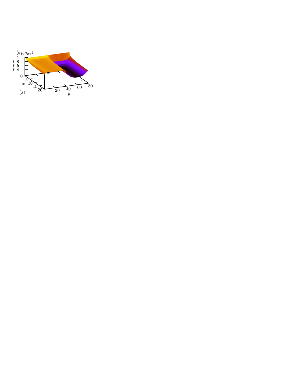
For the aspect ratio , we also sampled the spin-spin correlation functions and in - and -direction, respectively. In the ordered regime where nearly all spins are aligned in the same direction (, say) we find for and (where ) almost constant values near unity as one expects. The fast decay of the spin-spin correlation function to a slightly smaller value in the upper half of the system indicates that the interface is localized near the boundary, cf. Figure 5 (a). In the regime with an interface in the bulk along the -direction we find a symmetric shape of as a function of which is a clear signal for the phase separation, see Figure 5 (b). The opening angle between the plus and minus phases for and , respectively, is a measure for the fluctuations of the interface, e.g. a stiff interface shows an acute angle. For temperatures above the critical temperature, i.e. in the disordered phase, we observe a similar vanishing of the spin-spin correlation functions as in the pure 2D Ising model, see Figure 5 (c).
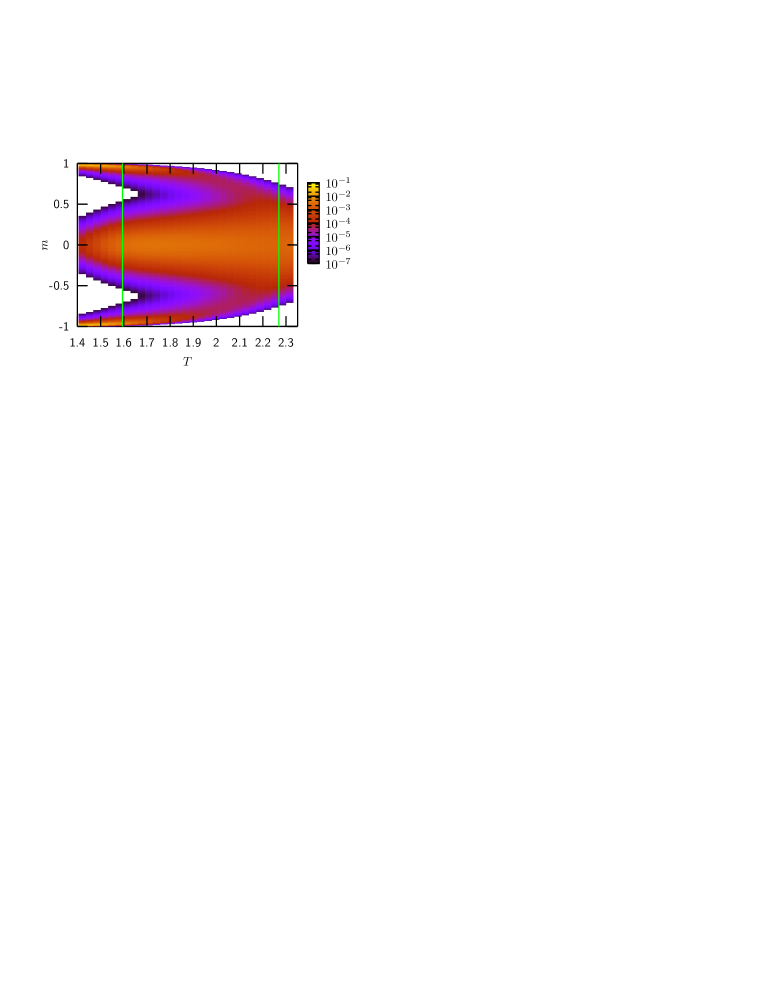
At zero temperature, for aspect ratios larger than the critical ratio and strong fields , the interface is localized on the boundary, cf. Figure 1. Although for no real solution of Equation (2) exists near , one can solve the equation for small temperatures111Here we are in disagreement with Ref. [9] where no solution was found, because of a mistake in the discriminant of Equation (2). and finds in the case the phase diagram shown in Figure 6. The zero temperature limit is consistent with the energetic arguments in Ref. [9], see also Figure 1. The lower line starting at , can also be detected by means of computer simulations, but as one can see in the right plot of Figure 6, for the dip between the two maxima in the boundary magnetization density vanishes with increasing lattice sizes. Therefore, there is no signal for a first-order transition between these two regimes. One can argue that there is no phase transition at all, because in the infinite-volume limit only the ordered phase survives. The dashed line in the left plot of Figure 6 starting at , is not visible in simulations, because this second solution of Equation (2) would correspond to the boundary between the bulk magnetized state and configurations with an interface propagating inside the bulk which, however, have a higher free energy then configurations with an interface localized near the boundary and hence are suppressed. Therefore the phase diagram for consists only of two phases, namely the ordered low-temperature phase and the disordered high-temperature phase as in the pure 2D Ising model. We hence conclude that for the inhomogeneous boundary magnetic field only leads to finite-size effects.
Finally, let us come to the special case of . While the transition line disappears for as the solutions of Equation (2) move to the complex plane, for we still do see different peaks associated with the two phases and, therefore, a finite interface tension, cf. Table 2. The numerically estimated transition points for and also contained in Table 2 are again seen to be in good agreement with Equation (2). Furthermore, we analysed for the spin-spin correlation functions and in - and -direction, respectively. Slightly below the transition from the ordered phase with to the phase with an interface propagating inside the bulk and therefore , shows an asymmetric shape and a fast decay near the boundary, indicating that the interface is localized near the boundary, cf. Figure 7 (a). With increasing boundary magnetic field we cross the first-order line at , where the interface starts moving into the bulk and, therefore, the profile of becomes symmetric in . Right at the transition line where we have two coexisting phases we find both the fast decay near the boundary as well as the opening angle between the two almost symmetric halves, see Figure 7 (b). When the boundary magnetic field is increased further, this mixed-phase effect vanishes and the interface in the bulk becomes stable. In this case we find a symmetric shape of the spin-spin correlation function, cf. Figure 7 (c), similar to in Figure 5 (b).
4 Summary
Our Monte Carlo data clearly confirm the theoretical considerations of Clusel and Fortin [9] and extend their exact results by studying the cases equal and larger than the critical value . The observed finite-size scaling behaviour fits nicely with their predictions for the infinite system, cf. our results in Table 2. We also find that for a large aspect ratio some interesting finite-size effects can be observed, such as, for example, a regime in the – plane with two states separated by an energy gap which vanishes in the infinite-volume limit. Furthermore, we studied the spin-spin correlation function for which analytical results are not yet available. Since this observable turned out to be quite sensitive to the interface location, it would be a challenging enterprise to pursue further analytical considerations in this direction.
Acknowledgments
We gratefully acknowledge financial support from the Deutsche Forschungsgemeinschaft (DFG) under Grant No. JA 483/23-1, the DFG Research Group FOR877, and the EU RTN-Network ‘ENRAGE’: Random Geometry and Random Matrices: From Quantum Gravity to Econophysics under Grant No. MRTN-CT-2004-005616.


References
References
- [1] J.W. Cahn, J. Chem. Phys. 66, 3667 (1977).
- [2] C. Ebner and W.F. Saam, Phys. Rev. Lett. 38, 1486 (1977).
- [3] H. Nakanishi and M.E. Fisher, J. Chem. Phys. 78, 3279 (1983).
- [4] B.M. McCoy and T.T. Wu, The Two-Dimensional Ising Model (Harvard Univ. Press, Cambridge, Mass., 1973).
- [5] A.B. Zamolodchikov, Adv. Stud. Pure Math. 19, 641 (1989); Int. J. Mod. Phys. A 4, 4235 (1989).
- [6] D.B. Abraham, Phys. Rev. Lett. 44, 1165 (1980); Phys. Rev. B 25, 4922 (1982); Phys. Rev. B 37, 3835 (1988).
- [7] H. Au-Yang and M.E. Fisher, Phys. Rev. B 11, 3469 (1975).
- [8] M. Clusel and J.-Y. Fortin, J. Phys. A 38, 2849 (2005).
- [9] M. Clusel and J.-Y. Fortin, J. Phys. A 39, 995 (2006).
- [10] W. Janke, Histograms and all that, in: Computer Simulations of Surfaces and Interfaces, NATO Science Series, II. Mathematics, Physics and Chemistry – Vol. 114, edited by B. Dünweg, D.P. Landau, and A.I. Milchev (Kluwer, Dordrecht, 2003); pp. 137–157.
- [11] B.A. Berg, J. Stat. Phys. 82, 323 (1996).
- [12] W. Janke, First-order phase transitions, in: Computer Simulations of Surfaces and Interfaces, NATO Science Series, II. Mathematics, Physics and Chemistry – Vol. 114, edited by B. Dünweg, D.P. Landau, and A.I. Milchev (Kluwer, Dordrecht, 2003); pp. 111–135.