Dynamic phase transition in the two-dimensional kinetic Ising model in an oscillating field: Universality with respect to the stochastic dynamic

Abstract

We study the dynamical response of a two-dimensional Ising model subject to a square-wave oscillating external field. In contrast to earlier studies, the system evolves under a so-called soft Glauber dynamic [P. A. Rikvold and M. Kolesik, J. Phys. A: Math. Gen. 35, L117 (2002)], for which both nucleation and interface propagation are slower and the interfaces smoother than for the standard Glauber dynamic. We choose the temperature and magnitude of the external field such that the metastable decay of the system following field reversal occurs through nucleation and growth of many droplets of the stable phase, i.e., the multidroplet regime. Using kinetic Monte Carlo simulations, we find that the system undergoes a nonequilibrium phase transition, in which the symmetry-broken dynamic phase corresponds to an asymmetric stationary limit cycle for the time-dependent magnetization. The critical point is located where the half-period of the external field is approximately equal to the metastable lifetime of the system. We employ finite-size scaling analysis to investigate the characteristics of this dynamical phase transition. The critical exponents and the fixed-point value of the fourth-order cumulant are found to be consistent with the universality class of the two-dimensional equilibrium Ising model. As this universality class has previously been established for the same nonequilibrium model evolving under the standard Glauber dynamic, our results indicate that this far-from-equilibrium phase transition is universal with respect to the choice of the stochastic dynamics.

I Introduction

Kinetic Ising or lattice-gas models with stochastic dynamics have been successfully applied to study a number of dynamical physical phenomena, including metastable decay Rikvold et al. (1994); Ramos et al. (1999); Berthier et al. (2004a, b); FRAN05 ; Frank and Rikvold (2006), hysteretic responses Sides et al. (1998, 1999); Korniss et al. (2001), and magnetization switching in nanoscale ferromagnets Richards et al. (1995); Novotny et al. (2002). Among the dynamic phenomena in such models that have attracted particular attention in recent years, is the dynamic phase transition (DPT) observed in systems with Ising-like symmetry that are driven far from equilibrium by an oscillatory applied force (typically a magnetic field or (electro)chemical potential). This phenomenon was first observed in kinetic simulations of a mean-field model Tomé and de Oliveira (1990); Mendes and Lage (1991) and later studied intensively by mean-field Zimmer (1993); BUEN98 ; Acharyya and Chakrabarti (1995); Chakrabarti and Acharyya (1999), Monte Carlo Lo and Pelcovits (1990); Acharyya and Chakrabarti (1995); Chakrabarti and Acharyya (1999); Sides et al. (1998, 1999); Korniss et al. (2001, 2002); Robb et al. (2007), and analytical Fujisaka et al. (2001); Tutu and Fujiwara (2004); Meilikhov (2004); Dutta (2004) methods. In this transition, the dynamic order parameter, which is the cycle-averaged magnetization, vanishes in a singular fashion at a critical value of the period of the applied field. Recently, strong experimental evidence has emerged that this nonequilibrium phase transition is observable in magnetic thin-film systems Robb et al. (2008), and an analogous phenomenon has been observed in simulations of a model of the heterogeneous catalytic oxidation of CO Machado et al. (2005); Buendía et al. (2006a).

Perhaps the most fascinating aspect of this far-from-equilibrium phase transition is that it belongs to the same universality class as the corresponding equilibrium Ising model. This result is predicted from symmetry arguments Grinstein et al. (1985); Bassler and Schmittmann (1994) and has been confirmed by exhaustive kinetic Monte Carlo simulations Sides et al. (1998, 1999); Korniss et al. (2001, 2002) and analytical results Fujisaka et al. (2001). Very recently, the field conjugate to the dynamic order parameter was identified as the cycle-averaged applied field, and a fluctuation-dissipation relation valid near the nonequilibrium critical point was numerically established Robb et al. (2007).

The physics of equilibrium phase transitions is well understood, and it is well established that structures arising from different dynamics that obey detailed balance and respect the same conservation laws exhibit universal asymptotic large-scale features. However, the mechanisms behind nonequilibrium phase transitions are not that well known, and the dependence on the specific dynamic is still an open question. Except for the study of the model of CO oxidation Machado et al. (2005); Buendía et al. (2006a), all previous kinetic Monte Carlo simulations in which this DPT was observed, were performed with the standard stochastic Glauber Glauber (1963) or Metropolis Metropolis et al. (1953) dynamics. All these studies, including the study of CO oxidation which used a very different dynamic, found critical exponent ratios consistent with the equilibrium Ising values, $\gamma/\nu=7/4$ and $\beta/\nu=1/8$. This gives a reasonable indication that this DPT is universal with respect to details of the model and the stochastic dynamics. However, a more direct test of just the universality with respect to the dynamics would be to use a significantly different stochastic dynamic for the two-dimensional kinetic Ising model. Such a test is the subject of the present paper.

All stochastic dynamics that respect detailed balance eventually lead to thermodynamic equilibrium Landau and Binder (2000), and all dynamics that obey the same conservation laws also give the same long-time dynamics (e.g., a $t^{1/2}$ dependence of the characteristic length for phase ordering with a non-conserved order parameter and a $t^{1/3}$ dependence for phase separation with a conserved order parameter Gunton et al. (1983)). However, it has recently been demonstrated that different stochastic dynamics give quantitatively dramatically different results for low-temperature nucleation Park et al. (2004); Buendía et al. (2004), as well as for the nanostructure and mobility of field-driven interfaces Rikvold and Kolesik (2002a, b, 2003); Buendía et al. (2006b, c). The differences are particularly striking between dynamics known as “hard,” in which the effects of the configurational and field-related (“Zeeman”) energy contributions in the transition rate do not factorize, and “soft,” for which such factorization is possible Rikvold and Kolesik (2002a); Park et al. (2004); Marro and Dickman (1999). The class of hard dynamics includes the standard Glauber and Metropolis dynamics, while the soft dynamics here will be represented by the “soft Glauber dynamic” introduced in Ref. Rikvold and Kolesik (2002a), whose transition rate is given in Sec. II. Briefly, the nanostructure of field-driven “hard” interfaces is characterized by a local interface width and mobility that increase dramatically with the strength of the applied field, while “soft” interfaces remain relatively smooth and slow-moving, independent of the field Rikvold and Kolesik (2002a). Similarly, low-temperature nucleation under hard dynamics becomes very fast for strong fields, while under soft dynamics it remains thermally activated and thus very slow, even for very strong fields Park et al. (2004). While the soft Glauber dynamic is probably not particularly relevant to any specific physical system, it is ideally suited for comparison with the standard, hard Glauber dynamic in investigating universal properties of the DPT.

The rest of this paper is organized as follows. The kinetic Ising model and its dynamics are introduced in Sec. II, and the numerical results and finite-size scaling analysis are presented in in Sec. III. A summary and conclusions are given in Sec. IV.

II Model and Dynamics

For this study we choose a kinetic, nearest-neighbor, Ising ferromagnet on a square lattice with periodic boundary conditions. The Hamiltonian is given by

$${\cal H}=-J\sum_{\langle ij\rangle}s_{i}s_{j}-H(t)\sum_{i}s_{i},$$ (1)

where $s_{i}=\pm 1$ is the state of the spin at the site $i$, $J>0$ is the ferromagnetic interaction, $\sum_{\langle ij\rangle}$ runs over all nearest-neighbor pairs, $\sum_{i}$ runs over all $L^{2}$ lattice sites, and $H(t)$ is an oscillating, spatially uniform applied field. The magnetization per site

$$m(t)=\frac{1}{L^{2}}\sum_{i=1}^{L^{2}}s_{i}(t),$$ (2)

is the density conjugate to $H(t)$. The temperature $T$ (in this paper given in units such that Boltzmann’s constant equals unity) is fixed below its critical value ($k_{B}T_{c}=J/\ln(1+\sqrt{2})$), so that, when there is no external field, the system has two degenerate equilibrium states with magnetizations of equal magnitude and opposite direction. When an external field is applied the degeneracy is lifted, and the equilibrium state is the one with magnetization in the same direction as the field. If the external field is not too strong, the state with opposite magnetization direction is metastable and eventually decays toward equilibrium Rikvold et al. (1994). This model is equivalent to a lattice-gas model with local occupation variables $c_{i}=(s_{i}+1)/2\in\{0,1\}$ and (electro)chemical potential $\mu\propto H$ (for further details, see Ref. Rikvold and Kolesik (2002b)).

The system evolves under the soft Glauber single-spin-flip (non-conservative) stochastic dynamic with updates at randomly chosen sites. In the lattice-gas representation, this corresponds to adsorption/desorption without lateral diffusion. The time unit is one Monte Carlo step per spin (MCSS). When the system is in contact with a heat bath at a temperature $T$, each proposed spin flip is accepted with probability

$$W_{\rm SG}=\frac{1}{1+\exp(\beta\Delta E_{J})}\frac{1}{1+\exp(\beta\Delta E_{H})}\;.$$ (3)

Here $\beta=1/T$, $\Delta E_{J}$ is the energy change corresponding to the interaction term, and $\Delta E_{H}$ is the energy change corresponding to the field term in the Hamiltonian, Eq. (1). This transition probability is to be contrasted with those of the standard, hard Glauber dynamic,

$$W_{\rm HG}=\frac{1}{1+\exp(\beta\Delta E)}\;,$$ (4)

and the Metropolis dynamic,

$$W_{\rm M}={\rm Min}[1,\exp(-\beta\Delta E)]\;,$$ (5)

where $\Delta E=\Delta E_{J}+\Delta E_{H}$ is the total energy change that would result from a transition.

The dynamical order parameter is the time-averaged magnetization over the $k$th cycle of the oscillating field Tomé and de Oliveira (1990),

$$Q_{k}=\frac{1}{2t_{1/2}}\int_{(k-1)2t_{1/2}}^{k2t_{1/2}}dt\,m(t)\;,$$ (6)

where $t_{1/2}$ is the half-period of the applied field. The cycle is chosen such that it starts when $H(t)$ changes sign. We also measured the normalized cycle-averaged internal energy,

$$\frac{E}{J}=-\frac{1}{2t_{1/2}}\int_{(k-1)2t_{1/2}}^{k2t_{1/2}}dt\frac{1}{L^{2}}\sum_{\langle ij\rangle}s_{i}(t)s_{j}(t)\;.$$ (7)

As previous studies indicate Sides et al. (1998, 1999); Korniss et al. (2001), the DPT transition essentially depends on the competition between two time scales: the average lifetime of the metastable phase, $\langle\tau(T,H_{0})\rangle$, and the half-period of the applied field, $t_{1/2}$. The metastable lifetime $\langle\tau\rangle$ is defined as the average time it takes the system to leave one of its two degenerate zero-field equilibrium states, when a field of magnitude $H_{0}$ opposite to the initial magnetization is applied. In practice the metastable lifetime is measured as the first-passage time to zero magnetization.

It is well known that metastable Ising models decay by different mechanisms depending on the magnitude of the applied field $H_{0}$, the system size $L$, and the temperature $T$. Detailed discussions of these different decays regimes are found in Ref. Rikvold et al. (1994). More recently it has also been shown that, contrary to some common beliefs, there is also a strong dependence on the specific stochastic dynamics Park et al. (2004); Buendía et al. (2004). For the purpose of this study the temperature, the system sizes and $H_{0}$ are chosen such that the metastable phase decays by random homogeneous nucleation of many critical droplets of the stable phase, which grow and coalesce, the so-called multidroplet (MD) regime. The metastable lifetime in the MD regime is independent of the system size Rikvold et al. (1994).

III Monte Carlo simulations

The numerical simulations reported in this work are performed on square lattices with $L$ between 64 and 256 at $T=0.8T_{c}$. The system is subjected to an square-wave field $H(t)$ of amplitude $H_{0}=0.3J$. The metastable lifetime was measured to be $\tau=145\pm 1$ MCSS, almost twice as long as for the kinetic Ising model evolving according to the standard (hard) Glauber dynamics under the same conditions Sides et al. (1998, 1999); Robb et al. (2007). This is consistent with earlier observations of slow nucleation Park et al. (2004) and interface growth Rikvold and Kolesik (2003) with this dynamic.

The system was initialized with all the spins up, and the square-wave external field started in the half-period in which $H=-H_{0}$. After the system relaxed, the magnetization and energy reached a limit cycle (except for thermal fluctuations), and all the period-averaged quantities became stationary stochastic processes. We discarded the first 2000 periods of the time series to exclude transients from the stationary-state averages.

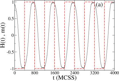
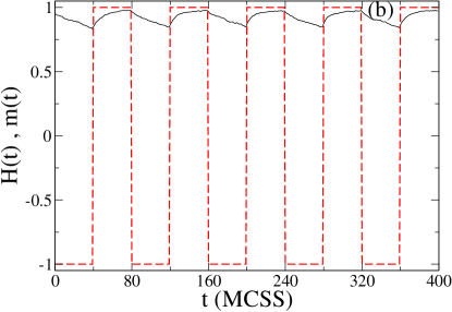
Figure 1: (Color online) Time series of the magnetization (solid curves) in the presence of a square-wave external field (dashed lines), for two values of the half-period $t_{1/2}$. (a) $t_{1/2}=400$ MCSS, corresponding to a dynamically disordered phase. (b) $t_{1/2}=40$ MCSS, corresponding to a dynamically ordered phase. The data were obtained for a system of size $L=128$ at $T=0.8T_{c}$ and field amplitude $H_{0}=0.3J$.

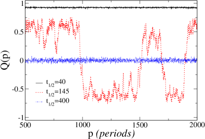
Figure 2: (Color online) Time series of the order parameter $Q$ for a system of size $L=128$ at $T=0.8T_{c}$ and $H_{0}=0.3J$. The horizontal trace near $Q=+1$ corresponds to a half-period of the field, $t_{1/2}=40$ MCSS, well into the dynamically ordered phase (see Fig. 1(b)). The strongly fluctuating trace corresponds to $t_{1/2}=145$ MCSS, very close to the DPT. The horizontal trace near $Q=0$ corresponds to $t_{1/2}=400$ MCSS, well into the dynamically disordered phase. (See Fig. 1(a)).

The time evolution of the magnetization is shown in Fig. 1. For slowly varying fields (Fig. 1(a)), the magnetization follows the field, switching every half-period. In this region, $Q\approx 0$. For rapidly varying fields (Fig. 1(b)), the magnetization does not have time to switch during a single half-period and remains nearly constant for many successive field cycles. As a result, the probability distribution of $Q$ becomes bimodal with two sharp peaks near the system’s spontaneous equilibrium magnetization, $\pm m_{\rm sp}(T)$, corresponding to the broken symmetry of the hysteresis loop. The transition between these two regimes is characterized by large fluctuations in $Q$. This behavior of the time series $Q_{k}$, shown in Fig. 2, is a clear indication of the existence of a dynamical phase transition between a disordered dynamic phase (the region where $Q\approx 0$), and an ordered dynamic phase (where $Q\neq 0$). Notice that the transition occurs at a critical value $\Theta_{\rm c}=t_{1/2}^{\rm c}/\tau$ that is very close to unity, the value at which the half-period of the external field is equal to the metastable lifetime of the system. To further explore the nature of the DPT, we perform a finite-size scaling analysis of the simulation data.

III.1 Finite-size scaling

Previous studies indicate that although scaling laws and finite-size scaling are tools designed for equilibrium systems with a well known Hamiltonian, they can be successfully applied to far-from-equilibrium systems like the one we are analyzing here Sides et al. (1998, 1999); Korniss et al. (2001); Machado et al. (2005); Robb et al. (2007).

Since for finite systems in the dynamically ordered phase the probability distribution of the order parameter is bimodal, in order to capture symmetry breaking, the order parameter is better defined as the average norm of $Q$, i.e., $\langle|Q|\rangle$. To characterize and quantify this transition by using finite-size scaling we must define quantities analogous to the susceptibility with respect to the field conjugate to the order parameter in equilibrium systems. The scaled variance of the dynamic order parameter,

$$\chi_{L}^{Q}=L^{2}(\langle Q^{2}\rangle_{L}-\langle|Q|\rangle_{L}^{2})\;.$$ (8)

has long been used as a proxy for the non-equilibrium susceptibility. A fluctuation-dissipation relation was recently demonstrated, which justifies this practice by connecting $\chi_{L}^{Q}$ to the susceptibility with respect to an applied bias field for a two-dimensional kinetic Ising model evolving under the standard Glauber dynamic Robb et al. (2007).

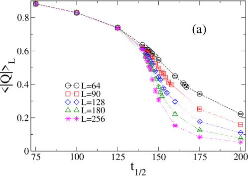
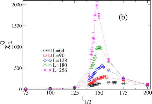
Figure 3: (Color online) Dependence on the half-period $t_{1/2}$ of the order parameter $\langle|Q|\rangle$ (a), and of its scaled variance $\chi_{L}^{Q}$ (b), shown for various system sizes, $L$. All the results correspond to $T=0.8T_{c}$ and $H_{0}=0.3J$.

In Fig. 3 we present the finite-size behavior of the order parameter and its fluctuations. Fig. 3(a) shows that this dynamic order parameter goes from unity to zero as $t_{1/2}$ increases, showing a sharp change around $t_{1/2}^{c}$, characterized by the peak in $\chi_{L}^{Q}$ shown in Fig. 3(b). The absence of finite-size effects below the critical point is the signature of the existence of a divergent length scale. The height and the location of the maximum in $\chi_{L}^{Q}$ change with $L$.

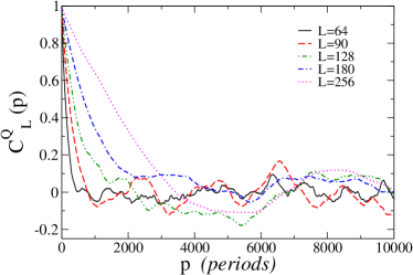
Figure 4: (Color online) Normalized autocorrelation function for the order parameter $Q$ for $t_{1/2}=145$ MCSS at $T=0.8T_{c}$ and $H_{0}=0.3J$, shown for different values of $L$.

In Fig. 4 we show the normalized time-autocorrelation function of the order parameter, defined as

$$C_{L}^{Q}(p)=\frac{\langle Q(i)Q(i+p)\rangle-\langle Q(i)\rangle^{2}}{\langle Q(i)^{2}\rangle-\langle Q(i)\rangle^{2}}.$$ (9)

The increasing correlation times with increasing system sizes are evidence of the critical slowing down of the system, and provides further support for the existence of a DPT.

We also measured the period-averaged internal energy, Eq. (7), and its scaled variance

$$\chi_{L}^{E}=L^{2}(\langle E^{2}\rangle_{L}-\langle E\rangle_{L}^{2})\;.$$ (10)

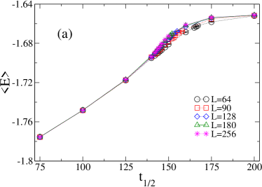
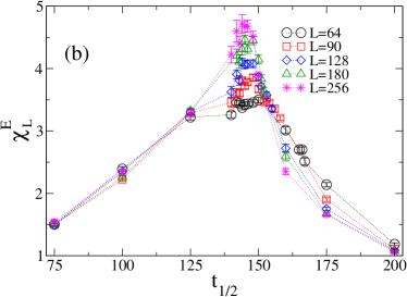
Figure 5: (Color online) Dependence on the half-period $t_{1/2}$ of the period-averaged internal energy $\langle E\rangle$ (a), and its scaled variance $\chi_{L}^{E}$ (b) for various system sizes, $L$. All the results correspond to $T=0.8T_{c}$ and $H_{0}=0.3J$.

Both quantities are shown in Fig. 5. Again, in the absence of a fluctuation-dissipation relation, we use the scaled variance as a proxy for the analog of the equilibrium heat capacity. The correlation time was used to estimate the proper sampling interval for estimating the fluctuation measures and their error bars as described in Ref. Landau and Binder (2000).

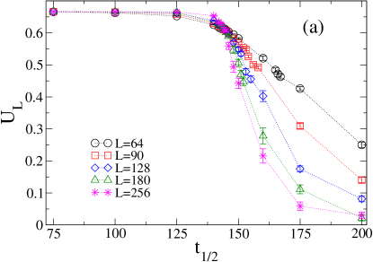
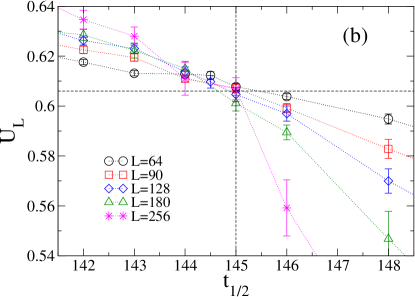
Figure 6: (Color online) (a) Dependence of the fourth-order cumulant $U_{L}$ on the half-period $t_{1/2}$, shown for various system sizes, $L$. (b) Enlargement of the region around the cumulant crossing. The horizontal and vertical dashed lines indicate the fixed point value $U^{*}\approx 0.606$ and the critical half-period, $t_{1/2}^{\rm c}=145$ MCSS, respectively. All the results correspond to $T=0.8T_{c}$ and $H_{0}=0.3J$.

It is very difficult to locate with precision the maxima of $\chi_{L}^{Q}$ and $\chi_{L}^{E}$ for the individual finite system sizes. A more accurate estimation of the critical point at which the transition occurs in an $\it{infinite}$ system can be obtained from the fourth-order cumulant intersection method. In Fig. 6 we plot the fourth-order cumulant $U_{L}$ defined as Landau and Binder (2000)

$$U_{L}=1-\frac{\langle Q^{4}\rangle_{L}}{3\langle Q^{2}\rangle^{2}_{L}}$$ (11)

as a function of $t_{1/2}$ for several system sizes. Our estimate is $t_{1/2}^{\rm c}=(145\pm 1)$ MCSS, with a fixed-point value $U^{*}=0.606\pm 0.004$ for the cumulant (Fig. 6(b)). The latter is consistent with the universal value for the two-dimensional equilibrium Ising model, $U^{*}=0.6106901(5)$ KAMI93 .

Finite size-scaling theory for equilibrium systems Privman and Fisher (1984); Privman (1990) predicts the following scaling forms at the critical point,

$$\langle|Q|\rangle_{L}\propto L^{-\beta/\nu},$$ (12)

$$\chi_{L}^{Q}\propto L^{\gamma/\nu},$$ (13)

which are also applicable to the far-from-equilibrium DPT Sides et al. (1998, 1999); Korniss et al. (2001); Robb et al. (2007). If the specific-heat critical exponent $\alpha=0$, as it is for the equilibrium Ising universality class, then we also expect the logarithmic divergence,

$$\chi_{L}^{E}\propto A+B\ln(L)\;.$$ (14)

These relations enable us to estimate the critical exponent ratios $\beta/\nu$ and $\gamma/\nu$ and verify the logarithmic divergence in the period-averaged internal energy fluctuations. In Fig. 7 we present the results obtained by plotting the logarithm of $\langle|Q|\rangle_{L}$ (Fig. 7(a)), the logarithm of $\chi_{L}^{Q}$ (Fig. 7(b)), and $\chi_{L}^{E}$ (Fig. 7(c)), in term of the logarithm of $L$ at $t_{1/2}^{\rm c}$. We also plot the peak of the fluctuations, $\chi_{L}^{Q}({\rm Peak})$ (Fig. 7(b)), and $\chi_{L}^{E}({\rm Peak})$ (Fig. 7(c)), since they asymptotically should follow the same scaling laws. After fitting the data with a weighted, linear least-squares algorithm, our estimates for the critical exponents are: $\beta/\nu=1.44\pm 0.06$, $\gamma/\nu=1.77\pm 0.04$ (from the data at $t_{1/2}^{\rm c}$ ), the data from $\chi_{L}^{Q}(Peak)$ gives $\gamma/\nu=1.79\pm.02$ which agree within statistical error. Also, the straight line in Fig. 7(c) gives evidence of the logarithmic divergence of $\chi_{L}^{E}$ at the critical point. These results, together with our estimate for $U^{*}$, give strong support to the hypothesis that the DPT observed is in the same universality class of the equilibrium two-dimensional Ising model.

IV Discussion and Conclusions

In this paper we have studied the dynamical response of a two-dimensional Ising model exposed to a square-wave oscillating external field. The system evolves under the so-called soft Glauber dynamic. In previous works it was established that, in the field and temperature regions when the metastable decay occurs via a multidroplet mechanism, this system evolving under a standard (hard) Glauber dynamics undergoes a continuous phase transition, with critical exponent ratios consistent with the equilibrium Ising values. The aim of the present study was to explore the universality of this far-from-equilibrium DPT with respect to the dynamics chosen to evolve the system.

Our numerical results clearly indicate the existence of a DPT in the multidroplet regime. The transition depends on the competition between two time scales: the half-period of the applied field and the metastable lifetime of the system. We found that the metastable lifetime of the system evolving under the soft Glauber dynamics is roughly twice that of the same system evolving under the standard Glauber dynamic. However, in both cases the transition occurs at a critical point where both times are of the same order of magnitude. If the half-period of the applied field increases much beyond the metastable lifetime, the system is in a dynamically disordered phase characterized by a vanishing dynamic order parameter. A study of the autocorrelation function of the order parameter at the critical point provides evidence of critical slowing down, showing increasing correlation times with increasing system sizes.

We applied the machinery of finite-size scaling, originally developed for equilibrium phase transitions, to estimate the critical point and the critical exponent ratios $\beta/\nu$ and $\gamma/\nu$ for system sizes between $64$ and $256$ at $T=0.8T_{c}$ and $H_{0}=0.3J$. Our estimates are $\beta/\nu\approx 1.44\pm 0.06$ and $\gamma/\nu\approx 1.77\pm 0.04$. These values are close to those of the two-dimensional equilibrium Ising model: $\beta/\nu=1/8=0.125$, $\gamma/\nu=7/4=1.75$. Furthermore, our data strongly indicate a slow logarithmic divergence with $L$ of the period-averaged energy fluctuations, consistent with the equilibrium Ising exponent $\alpha=0$. The fixed-point value of the fourth-order cumulant, $U^{*}$, is also close to its expected universal Ising value, near 0.611.

This study provides further evidence of the universality class of the dynamic phase transition in kinetic Ising systems driven by an oscillating field, extending its domain to systems that evolve under different stochastic dynamics that lead to interfaces with significantly different structures on the nanoscale.

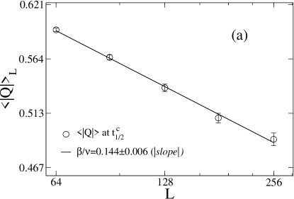
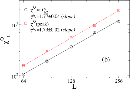
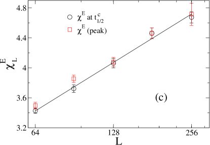
Figure 7: (Color online) Critical exponent estimates from the scaling relations. The symbols represent the MC data, the straight lines are weighted least-square fits. (a)Calculating $\beta/\nu$ from Eq. (12) calculating $\gamma/\nu$ from Eq. (13). (c) The logarithmic divergence of the period-averaged energy fluctuations, based on Eq. (14). From data at $t_{1/2}^{\rm c}=145$ MCSS, circles, at the peaks, squares.

References

- Rikvold et al. (1994) P. A. Rikvold, H. Tomita, S. Miyashita, and S. W. Sides, Phys. Rev. E 49, 5080 (1994).
- Ramos et al. (1999) R. A. Ramos, P. A. Rikvold, and M. A. Novotny, Phys. Rev. B 59, 9053 (1999).
- Berthier et al. (2004a) F. Berthier, B. Legrand, J. Creuze, and R. Tetot, J. Electroanal. Chem. 561, 37 (2004a).
- Berthier et al. (2004b) F. Berthier, B. Legrand, J. Creuze, and R. Tetot, J. Electroanal. Chem. 562, 127 (2004b).
- (5) S. Frank, D. E. Roberts, and P. A. Rikvold, J. Chem. Phys. 122, 064705 (2005).
- Frank and Rikvold (2006) S. Frank and P. A. Rikvold, Surf. Sci. 600, 2470 (2006).
- Sides et al. (1998) S. W. Sides, P. A. Rikvold, and M. A. Novotny, Phys. Rev. Lett. 81, 834 (1998).
- Sides et al. (1999) S. W. Sides, P. A. Rikvold, and M. A. Novotny, Phys. Rev. E 59, 2710 (1999).
- Korniss et al. (2001) G. Korniss, C. J. White, P. A. Rikvold, and M. A. Novotny, Phys. Rev. E 63, 016120 (2001).
- Richards et al. (1995) H. L. Richards, S. W. Sides, M. A. Novotny, and P. A. Rikvold, J. Magn. Magn. Mater. 150, 37 (1995).
- Novotny et al. (2002) M. A. Novotny, G. Brown, and P. A. Rikvold, J. Appl. Phys. 91, 6908 (2002).
- Tomé and de Oliveira (1990) T. Tomé and M. J. de Oliveira, Phys. Rev. A 41, 4251 (1990).
- Mendes and Lage (1991) J. F. F. Mendes and E. J. S. Lage, J. Stat. Phys. 64, 653 (1991).
- Zimmer (1993) M. Zimmer, Phys. Rev. E 47, 3950 (1993).
- (15) G. M. Buendía and E. Machado, Phys. Rev. E 58, 1260 (1998).
- Acharyya and Chakrabarti (1995) M. Acharyya and B. Chakrabarti, Phys. Rev. B 52, 6550 (1995).
- Chakrabarti and Acharyya (1999) B. Chakrabarti and M. Acharyya, Rev. Mod. Phys. 71, 847 (1999).
- Lo and Pelcovits (1990) W. S. Lo and R. A. Pelcovits, Phys. Rev. A 42, 7471 (1990).
- Korniss et al. (2002) G. Korniss, P. A. Rikvold, and M. A. Novotny, Phys. Rev. E 66, 056127 (2002).
- Robb et al. (2007) D. T. Robb, P. A. Rikvold, A. Berger, and M. A. Novotny, Phys. Rev. E 76, 021124 (2007).
- Fujisaka et al. (2001) H. Fujisaka, H. Tutu, and P. A. Rikvold, Phys. Rev. E 63, 036109 (2001); erratum: 63, 059903 (2001).
- Tutu and Fujiwara (2004) H. Tutu and N. Fujiwara, J. Phys. Soc. Jpn. 73, 2680 (2004).
- Meilikhov (2004) E. Z. Meilikhov, JETP Lett. 79, 620 (2004).
- Dutta (2004) S. B. Dutta, Phys. Rev. E 69, 066115 (2004).
- Robb et al. (2008) D. T. Robb, Y. H. Xu, A. Hellwig, A. Berger, M. A. Novotny, and P. A. Rikvold (2008), e-print arXiv:0705.4454.
- Machado et al. (2005) E. Machado, G. M. Buendía, P. A. Rikvold, and R. M. Ziff, Phys. Rev. E 71, 016120 (2005).
- Buendía et al. (2006a) G. M. Buendía, E. Machado, and P. A. Rikvold, J. Mol. Struct.: THEOCHEM 769, 189 (2006a).
- Grinstein et al. (1985) G. Grinstein, C. Jayaprakash, and Y. He, Phys. Rev. Lett. 55, 2527 (1985).
- Bassler and Schmittmann (1994) K. E. Bassler and B. Schmittmann, Phys. Rev. Lett. 73, 3343 (1994).
- Glauber (1963) R. J. Glauber, J. Math. Phys. 4, 294 (1963).
- Metropolis et al. (1953) N. Metropolis, A. W. Rosenbluth, M. N. Rosenbluth, A. H. Teller, and E. Teller, J. Chem. Phys. 21, 1087 (1953).
- Landau and Binder (2000) D. P. Landau and K. Binder, A Guide to Monte Carlo Simulations in Statistical Physics (Cambridge University Press, Cambridge, 2000).
- Gunton et al. (1983) J. D. Gunton, M. San Miguel, and P. S. Sahni, in Phase Transitions and Critical Phenomena, Vol. 8, edited by C. Domb and J. L. Lebowitz (Academic, London, 1983).
- Park et al. (2004) K. Park, P. A. Rikvold, G. M. Buendía, and M. A. Novotny, Phys. Rev. Lett. 92, 015701 (2004).
- Buendía et al. (2004) G. M. Buendía, P. A. Rikvold, K. Park, and M. A. Novotny, J. Chem. Phys. 121, 4193 (2004).
- Rikvold and Kolesik (2002a) P. A. Rikvold and M. Kolesik, J. Phys. A: Math. Gen. 35, L117 (2002a).
- Rikvold and Kolesik (2002b) P. A. Rikvold and M. Kolesik, Phys. Rev. E 66, 066116 (2002b).
- Rikvold and Kolesik (2003) P. A. Rikvold and M. Kolesik, Phys. Rev. E 67, 066113 (2003).
- Buendía et al. (2006b) G. M. Buendía, P. A. Rikvold, and M. Kolesik, Phys. Rev. B 73, 045437 (2006b).
- Buendía et al. (2006c) G. M. Buendía, P. A. Rikvold, and M. Kolesik, J. Mol. Struct.: THEOCHEM 769, 207 (2006c).
- Marro and Dickman (1999) J. Marro and R. Dickman, Nonequilibrium Phase Transitions in Lattice Models (Cambridge University Press, Cambridge, 1999).
- (42) G. Kamieniarz and H. W. J. Blöte, J. Phys. A: Math. Gen. 26, 201 (1993).
- Privman and Fisher (1984) V. Privman and M. E. Fisher, Phys. Rev. B 30, 322 (1984).
- Privman (1990) V. Privman, in Finite-Size Scaling and Numerical Simulation of Statistical Systems, edited by V. Privman (World Scientific, Singapore, 1990).