Infrared Imaging of SDSS Quasars:
Implications for the Quasar K correction

Abstract

We have imaged 45 quasars from the Sloan Digital Sky Survey (SDSS) with redshifts $1.85<z<4.26$ in $JHK_{s}$ with the KPNO SQIID imager. By combining these data with optical magnitudes from the SDSS we have computed the restframe optical spectral indices of this sample and investigate their relation to quasar redshift. We find a mean spectral index of $\langle\alpha_{o}\rangle=-0.55\pm 0.42$ with a large spread in values. We also find possible evolution of the form $\alpha_{o}=(0.148\pm 0.068)z-(0.964\pm 0.200)$ in the luminosity range $-28.0<M_{i}<-26.5$. Such evolution suggests changes in the accretion process in quasars with time and is shown to have an effect on computed quasar luminosity functions.

1 Introduction

The recent publication of large samples of quasars from the Sloan Digital Sky Survey (SDSS; Schneider et al., 2007) and the Two Degree Field QSO Redshift Survey (2QZ; Croom et al., 2004) allows the study of the evolution of the quasar population spanning long lookback times with large, homogenous catalogs of objects and the characterization of the quasar luminosity function (QLF). The Richards et al. (2006a) QLF formed from the SDSS Third Data Release Quasar Catalog (DR3QLF) is defined from 15,343 quasars over 1622 deg², spanning redshifts from $z=0$ to $5$ and reaching luminosities down to $M_{i}<-23$ in their lowest redshift bins. They find a peak in type 1 quasar activity between $z=2.2$ and $2.8$ and a general flattening of the slope of the bright-end QLF with increasing redshift. Hopkins et al. (2007) compute a bolmetric QLF, combining many quasars surveys, including the DR3QLF and the 2QZ. They find a peak in the quasar luminosity density at $z=2.15$ and an evolving QLF bright-end slope that becomes flatter at redshifts $z>3$.

One major difficulty in characterizing the evolution in quasar space densities is finding an appropriate way to calculate the absolute magnitudes of a survey sample and compare these magnitudes with other surveys, or even to objects within the same survey if it spans a large redshift range, i.e., how to calculate the appropriate K correction. Traditionally, absolute magnitudes were corrected back to the restframe $B$-band (Schmidt & Green, 1983; Boyle et al., 1987), as most early surveys for quasars included the measurement of flux around $4400\AA$, by assuming a power-law form for quasar spectra redward of Lyman-$\alpha$ of the form $f_{\nu}\propto\nu^{\alpha}$ and assuming an average spectral index, $\alpha$, for the survey sample. As surveys move to higher redshifts, beyond $z=3$, the observed $B$-band ceases to sample the quasar continuum effectively, as the Lyman-$\alpha$ line moves into and redward of that filter. In the recent past, research groups have adopted several methods for computing absolute magnitudes and have referenced their magnitudes to different restframe wavelengths. For instance, Schmidt, Schneider & Gunn (1995) and Kennefick et al. (1995) adopt an average spectral index of $\alpha=-0.5$ in their computations of $M_{B}$, while Warren, Hewett & Osmer (1994) avoid the adoption of a spectral index by computing the QLF as a function of $M_{C(1216)}$, the flux in the continuum under the Lyman-$\alpha$ line, from their direct measurements of the flux at that point in their survey spectra. More recently, Croom et al. (2004) present their QLF from the 2QZ at $0.4<z<2.1$ in terms of $M_{b_{J}}$, and Richards et al. (2006a) assume an average spectral index, but correct $i$-band magnitudes to $z=2$. The correction to $z=2$ is prompted by the desire to minimize the effects of extrapolating the assumed quasar powerlaw over large wavelengths, as suggested by Wisotzki (2000).

Such differences in the methods for computing absolute magnitudes has led to some discrepancies in computed quasar space densities in past surveys (Kennefick et al., 1997). The initial goals of this near-infrared (NIR) imaging program were to measure the restframe $B$-band flux for a set of quasars in several redshift ranges, to compare the differences in the absolute magnitudes, $M_{B}$, as computed from extrapolations of flux values at lower wavelengths to flux values measured directly, and to see how this changed with redshift. This is equivalent to measuring the restframe optical spectral index of the quasars from optical and NIR photometry. In this paper we report the initial results of a program to measure the restframe optical spectral index, $\alpha_{o}$, of a subset of SDSS quasars at $1.85<z<4.26$ using their reported optical magnitudes and NIR photometry obtained at the KPNO 2.1m telescope using the Simultaneous Quad Infrared Imaging Device (SQIID). In §2 we present the program design. The data used in the project, both archived and new observations, are described in §3. In §4 we give the program results, including computations of spectral indices and the implications for the resulting absolute magnitudes. We discuss our results further in §5.

2 Program Design

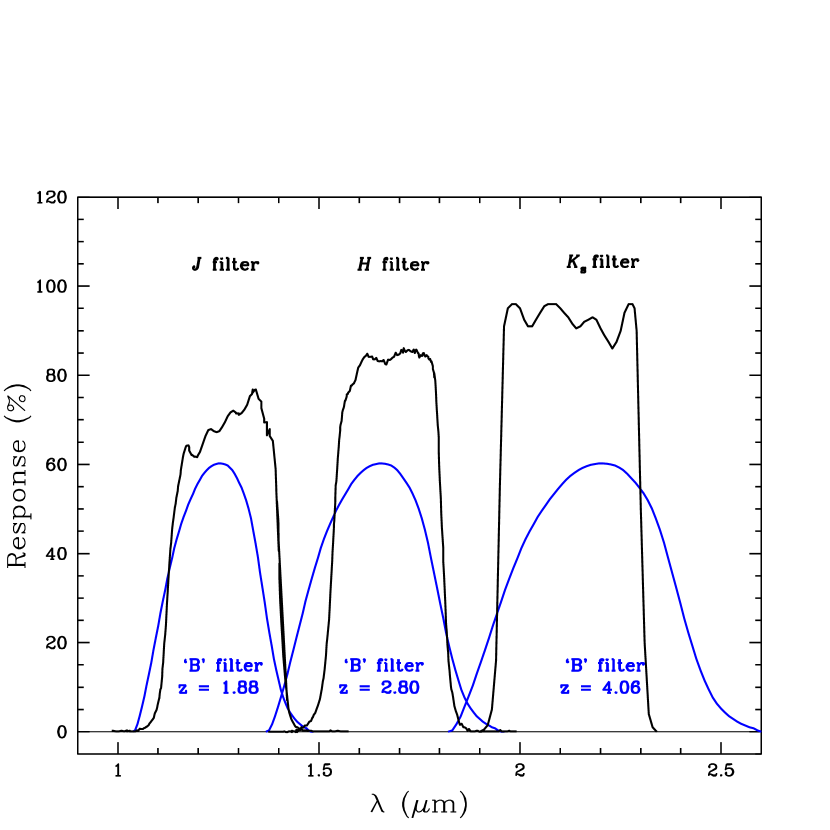
Figure 1: SQIID $JHK_{s}$ filters along with the Johnson $B$ filter “redshifted” to show where the restframe $B$-band flux of quasars at the given redshift would be with respect to the corresponding SQIID NIR filter.

The initial goal of this observing program was to measure the restframe $B$-band flux for a sample of quasars at a range of redshifts in order to essentially bypass the need to extrapolate a power-law over large wavelength ranges when applying a K correction in the computation of quasar absolute magnitudes, $M_{B}$. The central wavelength of the $J$-band is 1.27 microns, which corresponds to the restframe $B$-band (central wavelength of 4400 $\AA$) at $z=1.88$. Likewise, $H$-band corresponds to the restframe $B$-band at $z=2.80$, and $K_{s}$-band at $z=4.06$. Figure 1 shows the NIR $JHK_{s}$ filter curves, along with the “redshifted” Johnson $B$-band at these redshifts, that is, the portion of the spectrum you would like to measure to sample the restframe $B$-band at the given redshift. For this project, we targeted 45 quasars chosen from the SDSS quasar catalogs for NIR imaging centered around the above redshift ranges. We combine this NIR photometry with reported optical magnitudes to compute restframe optical spectral indices for the sample. Programatically, this can be achieved by fitting the photometric data to measure the slope of the spectral energy distribution, $\alpha$, as dicussed further below.

Richards et al. (2006a) has reported the DR3QLF computed from SDSS quasars as a function of $M_{i}$ corrected to a redshift of $z=2$, and the selection of the $B$-band for computations of the QLF has become less common as quasar surveys move to higher redshift. Here, we compute the optical spectral index, $\alpha_{o}$, for a subset of the SDSS quasars using optical and NIR photometry. We then explore possible correlations of $\alpha_{o}$ with redshift or luminosity and how that might affect the characterization of the QLF and its evolution.

3 Observations and Data Reductions

3.1 SQIID Near-Infrared Imaging

Forty-five quasars from the SDSS Third Data Release Quasar Catalog (DR3Q; Schneider et al., 2005) were imaged with SQIID on the KPNO 2.1m telescope during 2005 March 22-23. The SQIID Infrared Camera uses individual $512\times 512$ pixel quadrants of ALADDIN InSb arrays, with a pixel scale of 0.69″pixel^-1 at the KPNO 2.1m. The effective field of view is 304″$\times$ 317″. We configured SQIID to take images in the $JHK_{s}$ bands, which it acquires simultaneously by splitting the beam with a series of dichroics before sending the beam to separate NIR cameras optimized to perform over a limited wavelength range.

The observing strategy involved imaging each target quasar for a total of 600s, with five pointings of 120s, each the sum of fifteen 8s coadds, offset by roughly 45″ between pointings to improve background subtraction. Conditions were nonphotometric, with light cirrus over the course of the run. Seeing ranged from 1.3″ to 1.9″ over the two nights of the observing run.

The images were processed using the IRAF UPSQIID package. Dark frames were acquired for each combination of coadd and exposure time utilized during the run. A global flatfield for each night and each filter was constructed from the object frames using the USQFLAT routine, configured to subtract the dark current and then to perform a median combine of the frames. Image processing was performed using the MOVPROC routine to generate and subtract a moving sky image created from the 6 frames obtained closest to the object frame in time and to correct for pixel to pixel sensitivity differences by dividing by the appropriate flatfield. The final image of each quasar in each band was constructed by registering the five pointings using the USQMOS routines and combining the frames using the NIRCOMBINE routine.

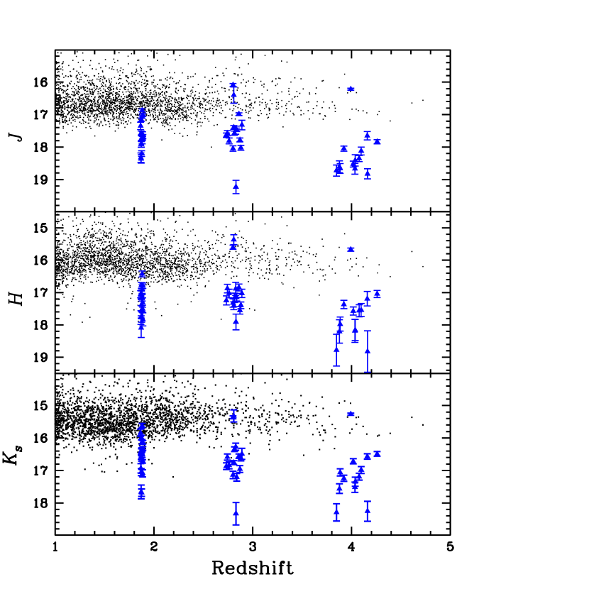
Figure 2: SQIID $JHK_{s}$ magnitudes for the sub-sample of SDSS quasars given in Table 1 (blue triangles) along with their associated errors. Also shown are the $JHK_{s}$ magnitudes of the 6192 quasars from the SDSS Third Data Release Quasar Catalog (Schneider et al., 2005) with measurable 2MASS detections (black dots). The SQIID data reach about $1^{m}$ to $2^{m}$ fainter than the 2MASS data.

Object detection and measurement was carried out using the Source Extractor software. The observations were made under fair but nonphotometric conditions. Calibration was performed through the use of stellar Two Micron All Sky Survey (2MASS; Cutri et al., 2003) sources in the object frames. The 2MASS images and catalogs were accessed through the National Virtual Observatory (NVO) Open SkyQuery and DataScope Query tools and manipulated using the Aladin multiview tool (Bonnarel et al., 2000). The $JHK_{s}$ magnitudes reported in Table 1 and used in the following analysis were derived from the flux inside circular apertures of radius 3.5″. The photometric zeropoints for the frames were calculated using stellar 2MASS sources in the frame of the quasar with measured $JHK_{S}$ aperture magnitudes. Typically five to seven calibration stars were used with magnitudes ranging from 14 to 16 in $J$ and $H$, and from 14 to 15 in $K_{s}$. The 2MASS aperture magnitudes were measured in a 4″ radius and “curve-of-growth” corrected out to an “infinite” aperture. Therefore, the magnitudes given in Table 1 are effectively aperture corrected by using these corrected 2MASS sources as standards. Near-infrared magnitudes, uncorrected for Galactic extinction, for the quasars are given in Table 1 and Figure 2, along with their associated errors, which include both measured photometric errors for the quasars and the errors introduced by the calibration process. The quasars in the subsample observed with SQIID are 1 to 2 magnitudes fainter than the SDSS quasars detected by 2MASS. The relatively few numbers of quasars in the highest redshift bin ($\sim 4.06$) meant that we had to choose fainter objects over a slightly wider redshift range than in the two lower redshift bins.

3.2 The SDSS Third Data Release Quasar Catalog

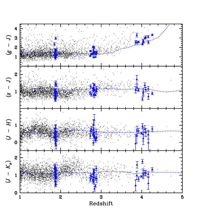
Figure 3: SDSS optical and SQIID $JHK_{s}$ colors for the sub-sample of SDSS quasars observed with SQIID given in Table 1 (blue triangles) along with their associated errors. Also shown are the colors of the 6192 quasars from the SDSS Third Data Release Quasar Catalog with measurable 2MASS detections (black dots). The dashed line shows the expected colors of quasars with spectral indices of $\alpha=-0.5$, including emission lines and Lyman-$\alpha$ forest continuum depression.

The SDSS uses a multicolor technique to select quasar candidates in the optical $ugriz$ bands over the redshift range $0.08<z<5.41$. The DR3Q contains 46,420 quasars with luminosities $M_{i}>-22$. Initially, we chose 60 quasars from the SDSS Early Data Release quasar catalog (EDR; Schneider et al., 2002) for NIR imaging. Quasars were selected from the EDR catalog randomly from those objects with r.a. between $9^{h}$ and $16^{h}$ and as close to the target redshifts as possible. Since the EDR contains more objects at lower redshifts, there is less spread in the sample redshifts at $z=1.88$, increasing slightly at $z=2.80$ and more pronounced at $z=4.06$ (see Figures 2 and 3). The mean redshifts for the three bins are $z=1.88$, $2.82$, and $4.03$. We obtained NIR imaging for 45 of these objects, chosen to sample our redshift ranges and with RA’s close to the local sidereal time during the observations. All of the imaged quasars are contained in the SDSS DR3Q catalog, and the optical photometry reported in Table 1 and used in the data analysis were taken from this later catalog.

The SDSS DR3Q has been matched to the 2MASS All-Sky Data Release Point Source Catalog (Cutri et al., 2003) and the 2MASS $JHK_{s}$ magnitudes and errors are reported for those SDSS quasars with 2MASS detections (columns 25-30 of the DR3Q.) We have used the 6192 quasars with 2MASS detections as a bright comparison sample to our fainter (1^m to 1.5^m) SQIID sample (Figures 2 and 3).

4 Results

4.1 Colors

The magnitudes were corrected for Galactic extinction using the value of $A_{u}$ for each object reported in the SDSS DR3Q catalog, column 15 (Schneider et al., 2005). These values were taken from the maps of Schlegel et al. (1998) which assumes an extinction to reddening ratio $R_{V}=3.1$. Extinctions in the Sloan $griz$ bands are then 0.736, 0.534, 0.405, and 0.287 times $A_{u}$, respectively. The value of $A/E(B-V)$ for the Sloan $u$-band is 5.155; consulting Schlegel et al. (1998) for the UKIRT $JHK$ values gives 0.902, 0.576, and 0.367, respectively. This gives values for the extinction in these bands of $A_{J}=0.175A_{u}$, $A_{H}=0.112A_{u}$, and $A_{K}=0.071A_{u}$. Colors computed from these extinction corrected magnitudes for the SQIID sample and the SDSS quasars detected by 2MASS are shown in Figure 3. The SQIID sample spans the same range in quasar colors as do the 2MASS detected quasars.

Also shown in Figure 3 are expected colors for quasars computed using synthetic quasar spectra generated with power law spectral indices and averaged over several different realizations of the Lyman-$\alpha$ forest. The colors were computed by passing the quasar spectra through SDSS and SQIID filters and calibrated with a comparison Vega spectrum from the Space Telescope Science Institute CALSPEC site. The $ugriz$ Vega based magnitudes were then converted to the SDSS $AB$ system using Holberg & Bergeron (2006). The dotted line in Figure 3 represents quasars with $\alpha=-0.5$. While the quasar colors do cluster around this line, the colors span a considerable range, larger than the errors in their colors. This is consistent with results found by Pentericci et al. (2003), who found a similar spread in optical/NIR colors in a sample of 45 SDSS quasars at $3.6<z<5.03$.

4.2 Optical Spectral Indices

In order to compute the restframe optical continuum slopes of the quasar spectral energy distributions, we have converted our NIR, Vega based photometry to the AB system. To accomplish this, we first constructed a NIR spectrum for Vega based on the absolute flux calibrations for Vega reported by Mégessier (1995) (see their Table 4,) constraining the blue end to have $f_{\nu}=2446JY$ at $\lambda=9000\AA$, as given in their formula for the blackbody fit to Vega (see their page 776.) We then compared the flux from this spectrum with a flat source with $f_{\nu}=3631Jy$, the zeropoint of the AB system (Oke & Gunn, 1983), for each 2MASS and SQIID $JHK_{s}$ filter. The offsets for the 2MASS filter set are: $J_{AB}=J+0.84$, $H_{AB}=H+1.33$, and $K_{AB}=K_{s}+1.79$. For the SQIID filter set they are: $J_{AB}=J+0.88$, $H_{AB}=H+1.35$, and $K_{AB}=K_{s}+1.75$.

If we assume that the optical flux for a quasar is given by $f_{\nu}=\nu^{\alpha_{o}}$, then we can rewrite the formula for the AB magnitude (Oke & Gunn, 1983)

$$AB=-2.5\log_{10}f_{\nu}-48.6$$ (1)

in the following form:

$$AB=-2.5\alpha_{o}\log_{10}\nu-48.6,$$ (2)

allowing us to compute $\alpha_{o}$ as the slope of a fit to straight line in AB magnitude vs. $\log\nu$. This was accomplished by using the Numerical Recipes routine FIT (Press et al., 1992). Spectral indices for each quasar observed with SQIID are given in Table 2. The mean spectral index for the sample is $\langle\alpha_{o}\rangle=-0.55\pm 0.42$. However, there appears to be a change in the mean slope with redshift in the SQIID sample, with quasars at lower redshifts having a steeper slope. In Figure 4, AB magnitudes transformed to the quasar restframe and normalized to 20.0 in the bluest band completely redward of Lyman-$\alpha$ are given along with a line showing the mean slope for that redshift range. The mean spectral index for each of the redshift bins is: $\langle\alpha_{o}\rangle_{1.88}=-0.71\pm 0.43$, $\langle\alpha_{o}\rangle_{2.82}=-0.49\pm 0.40$, $\langle\alpha_{o}\rangle_{4.03}=-0.40\pm 0.39$ (see also Table 3). These spectral indices were calculated using all available passbands. For consistency, if we only use those passbands available in all three redshift bins (from restframe $\sim 1500\AA$ out to $\sim 4500\AA)$, the computed spectral indices change very little, with means of: $\langle\alpha_{o}\rangle_{1.88}=-0.68$, $\langle\alpha_{o}\rangle_{2.82}=-0.50$, $\langle\alpha_{o}\rangle_{4.03}=-0.40$.

4.3 K corrections and Absolute Magnitudes

In order to compute a luminosity function for quasars, the absolute magnitude of each discovered object must be calculated. This can be a bolometric luminosity, the luminosity at a point in the continuum, or the flux in a passband. However, since the spectra of quasars are redshifted and even an individual survey can span a large range in redshift, the calculation must include a conversion from an observed band to an emitted band. This conversion from observed flux to restframe flux is referred to as the K correction (Humason, Mayall, & Sandage, 1956), defined as the “technical effect that occurs when a continuous energy distribution $F(\lambda)$ is redshifted through fixed spectral-response bands of a detector” (Oke & Sandage, 1968). If the spectral energy distribution (SED) is not flat, this will include both the effect of detecting light from a region of the emitted spectrum shifted from the effective wavelength of the detector and the effective squeezing of the detector bandpass in the emitted frame.

Following the formalism of Hogg et al. (2002), the K correction is defined as

$$M_{emitted}=m_{observed}-DM-K(z),$$ (3)

where $DM$ is the distance modulus, given as

$$DM=5\log_{10}\left[{D_{L}\over 10{\rm pc}}\right],$$ (4)

$K(z)$ is the K correction, which depends on the SED of the observed object (see Hogg et al., 2002, eq. 8), and $D_{L}$ is the luminosity distance. Following Hogg (2000) and assuming $\Omega_{M}+\Omega_{\Lambda}=1$, the luminosity distance is given by

$$d_{L}(z;\Omega_{M},\Omega_{\Lambda},H_{0})={c(1+z)\over H_{0}}\times$$

$$\int_{0}^{z}[(1+z^{\prime})^{2}(1+\Omega_{M}z^{\prime})-z^{\prime}(2+z^{\prime})\Omega_{\Lambda}]^{-1/2}dz^{\prime}.$$ (5)

We assume $H_{0}=$70km s^-1 Mpc^-1, $\Omega_{M}=0.3$, and $\Omega_{\lambda}=0.7$ throughout (Spergel et al., 2007).

For a power-law SED of the form $f_{\nu}\propto\nu^{\alpha}$ we can write

$$K(z)=-2.5\alpha\log(1+z)-2.5\log(1+z)$$ (6)

where the first term transforms from the emitted band to the observed band at z=0 and the second term corrects for the effective narrowing of the passband when observing redshifted objects. Quasar spectra also contain various broad emission lines, and their contribution to the K correction will be addressed below.

Table 2 (column 4) lists the absolute magnitude, $M_{i(z=0)}$, for each quasar as reported in the SDSS DR3Q catalog. These values were computed by correcting the SDSS $i$ magnitudes for Galactic extinction, assuming $H_{0}=$70km s^-1 Mpc^-1, $\Omega_{M}=0.3$, and $\Omega_{\lambda}=0.7$, and applying a standard continuum K correction by assuming a spectral index of $\alpha=-0.5$ and correcting to $z=0$.

The DR3QLF is computed as a function of $M_{i}$, but $K$ corrected to $z=2$, near the peak in the quasar distribution. They also correct for emission lines by convolving a composite spectrum created from 16,713 SDSS quasars with the continuum subtracted with the SDSS filters. Their values are reported in Table 2 (column 5) as $M_{i(z=2)}$. They compute a combined K correction, assuming a spectral index of $\alpha=-0.5$ (see their Table 4), which we will refer to here as $K_{2}$. We adopt the Richards et al. (2006a) methodology but employ the spectral index computed for our SQIID subsample in computing the $M_{i}$. This gives an expression for $K(z)$:

$$K(z)=K_{2}-2.5(\alpha_{o}-\alpha_{fix})\log_{10}(1+z)$$ (7)

where $\alpha_{fix}=-0.5$. Therefore $M_{i(\alpha_{o})}$ is given as

$$M_{i(\alpha_{o})}=m_{i}-5\log_{10}\left[D_{L}\over 10{\rm pc}\right]\\ -K_{2}+2.5(\alpha_{o}+0.5)\log_{10}(1+z).$$ (8)

The values of $\alpha_{o}$ and $M_{i(\alpha_{o})}$ for the SQIID sample are listed in Table 2 (columns 6 and 8), and the $M_{i(\alpha_{o})}$ are plotted vs. redshift in Figure 5. Because our imaged $z\sim 4$ quasars are fainter than those in the two lower redshift ranges, the program samples quasars of similar luminosity at all three redshifts, unlike the 2MASS crossmatches, which have a distinct dependence of luminosity on redshift, as would be expected for a flux limited survey.

4.4 Correlations

In order to investigate possible correlations of $\alpha_{o}$ with redshift or luminosity, we used the Astronomy SURVival Analysis tools (ASURV; LaValley et al., 1992), accessed through the IRAF STSDAS package. Linear regressions were performed using both the EM (estimate and maximize; Dempster et al., 1977) and the Buckley-James (Buckley & James, 1979) algorithms resulting in the following expressions for $\alpha_{o}$ in terms of $z$ and $M_{i(\alpha_{o})}$:

$$\alpha_{o}(z)=(0.148\pm\ 0.068)z-(0.964\pm\ 0.200)$$ (9)

$$\alpha_{o}(M_{i(\alpha_{o})})=(0.168\pm\ 0.083)M_{i(\alpha_{o})}+(4.084\pm\ 2.305)$$ (10)

$$\alpha_{o}(z,M_{i(\alpha_{o})})=(0.249\pm\ 0.065)z+(0.295\pm\ 0.080)M_{i(\alpha_{o})}+(6.891\pm\ 2.137).$$ (11)

The expressions for $\alpha_{o}(z)$ and $\alpha_{o}(M_{i(\alpha_{o})})$ are plotted along with the data in Figure 6. We have also computed the generalized Kendall’s tau correlation coefficent between these variables using the BHK method (LaValley et al., 1992). For the $\alpha_{o}$ and $z$ relation, we find $\tau=0.40$ with a 95% probability of a correlation. For $\alpha_{o}$ and $M_{i(\alpha_{o})}$, we find $\tau=0.30$ with an 85% probability of a correlation. We note, however, that the SQIID sample was not chosen to sample a broad range of absolute magnitude. Instead fainter sources were necessarily chosen at higher redshifts because fewer bright quasars are present at these very high redshifts in the SDSS sample due to the relatively fewer numbers of quasars at these epochs. We have also included an expression for $\alpha_{o}(z,M_{i(\alpha_{o})})$ and show the projections of the residuals of this fit along with the residuals from the expressions for $\alpha_{o}(z)$ and $\alpha_{o}(M_{i(\alpha_{o})})$ in Figure 7. The residuals in the two-dimensional expressions (top panels) are similar to those for the three-dimensional expression (lower panels).

The distributions of the spectral indices for the SQIID and 2MASS detected samples are shown in Figure 8 (left panel). Also shown are the separate distributions of the SQIID subsamples at $z\sim 1.88$, $2.82$, and $4.03$ (right panel). The $\alpha_{o}$ of the 2MASS detected SDSS quasars were computed using the same method as for the SQIID sample, using the optical bands completely redward of Lyman-$\alpha$ and the available 2MASS data from the DR3Q. Sample statistics are given in Table 3. The median of the complete SQIID sample distribution is flatter than the mean with a value of $-0.47$. The mean is shifted to steeper values by the presence of a red tail to the distribution. The median of the 2MASS sample distribution is $-0.57$. The mean is again shifted redward by a red tail to $\langle\alpha_{o}\rangle=-0.70\pm 0.53$. The distributions of the two samples look very similar. However, performance of a Kolmogorov-Smirnov (K-S; Babu & Feigelson, 1996; Press et al., 1992) test on the two data sets shows only a 38% probability that the two distributions are drawn from the same parent distribution. The differences could be due to dependence of $\alpha$ on luminosity, as has been suggested by this work and others (e.g. Steffen et al., 2006), as the SQIID and 2MASS samples cover different areas of luminosity/redshift space (Figure 5.) If we consider just those quasars from the 2MASS sample with $-28<M_{i(\alpha_{o})}<-26.5$ (where the bulk of the SQIID sample lies), then the mean of the distribution is $\langle\alpha_{o}\rangle=-0.54\pm 0.37$ and the median is -0.47, almost identical to the SQIID sample, even though the bulk of these quasars are at redshifts between 0.5 and 2 (Table 3).

As is clear from Figure 5, the 2MASS detected sample has a strong correlation of luminosity with redshift. While this is also true, to a lesser degree, for the SQIID sample, in order to select a statistically significant sample at high redshift and stay close to our desired redshift ranges, we had to observe fainter candidates at the higher redshift bins, as can be seen in Figure 2. This resulted in the SQIID subsamples having very similar mean luminosities of $M_{i(\alpha_{o})}=-27.15$, $-27.89$, and $-27.87$ at $z\sim 1.88$, $2.82$, and $4.03$, respectively. It is therefore not surprising that we see stronger evidence in favor of a correlation of $\alpha_{o}$ with $z$ than with luminosity, as our survey was designed to explore the relation with redshift. We do note, however, that if we limit the 2MASS detected sample to have similar absolute magnitudes to our sample, then the statistics for $\alpha_{o}$ become very similar (Table 3), even though the mean reshifts are $1.44$ and $2.81$. What we conclude is that there is evidence for evolution of $\alpha_{o}$ with both $z$ and luminosity, but that more data at a broader range of luminosities is needed to fully characterize its form.

Computing the difference in the absolute magnitudes in Table 2, one computed with an average spectral index as in Richards et al. (2006a), $M_{i(z=2)}$, and another where the value of $\alpha_{o}$ is used, $M_{i(\alpha_{o})}$, we can see in Figure 9 that there is a trend with redshift, due to the suggested evolution of $\alpha_{o}$ with redshift. When using a spectral index computed from the quasar photometry, the quasars at $z\sim 2$ are brighter on average with respect to the luminosity computed with $\alpha=-0.5$, while the quasars at $z\sim 4$ are fainter. The difference in computed luminosities in the SQIID sample can be as much as $\pm 1\fm 8$.

4.5 The Quasar Luminosity Function

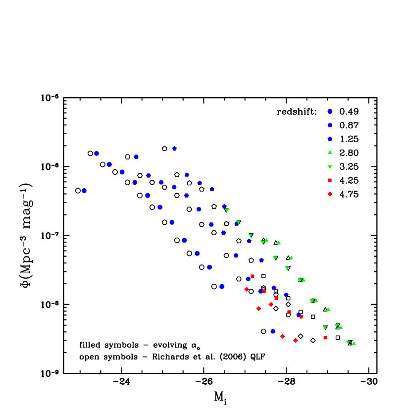
Figure 10: The QLF of Richards et al. (2006a) (black open symbols) and the same QLF but with the $M_{i}$ of the redshift bins calculated using an evolving $\alpha$ as given by Equation 9 and using the mean redshift of the quasars in the bin (colored filled symbols). Lower redshift quasars are found to be brighter and high redshift quasars are found to be fainter. This results in a steeper form for the evolution in quasar space densities.

If there is evolution in $\alpha$ with redshift or luminosity, this will have a direct effect on the evolution of the QLF. For example, the DR3QLF is shown in Figure 10 (open symbols). If we recompute the absolute magnitudes of the bins (see Richards et al., 2006a, Table 6) by using the mean redshift of the quasars in the bin in our Eq. 9 to compute an average $\alpha_{o}$ at this mean redshift, the absolute magnitudes will shift by an amount $\Delta M_{i}=2.5(\alpha_{o}+0.5)\log_{10}(1+z)$. This term will be zero where $\alpha_{o}=-0.5$, which corresponds to $z=3.1$. For redshifts significantly below this, the quasar SED is steeper on average, and $M_{i}$ is correspondingly brighter. For redshifts above $3.1$, the SED’s are on average flatter, and the $M_{i}$ are fainter.

This is shown graphically in Figure 10 where the DR3QLF is given along with points shifted in $M_{i}$ as described above. While the space density remains essentially unchanged near the peak of quasar activity at $z\sim 3$, the points shift towards brighter $M_{i}$ at lower redshift and towards fainter $M_{i}$ at higher redshifts. For cummulative space densities as a function of redshift, this would mean that at lower redshifts, more objects would have $M_{i}$ brighter than a given cutoff, increasing space densities, while at $z\sim 4$, fewer objects would make the cutoff, resulting in lower space densities. This would change the shape of the form in the number of quasars over time, giving rise to steeper growth at early times, with a more gradual decline locally.

5 Discussion

It has long been recognized that adopting an average spectral index for the power-law form of quasar spectral energy distributions can effect the evolution in the QLF (e.g. Giallongo & Vagnetti, 1992; Francis, 1996; Kennefick et al., 1997; Wisotzki, 1998; Richards et al., 2006a). However, the adoption of an average spectral index persists in most studies of the QLF, with $\alpha=-0.5$ being the most common value used. Recent work in the X-ray region has led to a general consensus that there is a dependence of quasar SED on luminosity (see Tang et al., 2007, for an exception). As for dependence on $z$, some groups find no evidence for the evolution of X-ray spectral indices, $\alpha_{ox}$, with redshift (e.g. Steffen et al., 2006), while others do see a linear dependence of optical to X-ray spectral indices with $z$ (Kelly et al., 2007). X-ray emission in AGN is generally taken to arise from a hot corona of optically thin gas heated by Compton scattering of thermal photons from a thick accretion disk, the likely source of the optical/UV emission. While emission from these two regions is likely related, there is little evidence for a direct link between the X-ray and optical/UV emission, and Kelly et al. (2007) find no evidence for a correlation between $\alpha_{UV}$ and $\alpha_{ox}$.

Previous attempts to study the optical spectral energy distributions of quasars include Francis (1996) who find $\alpha=-0.46\pm 0.30$ from a sample of LBQS quasars using optical and NIR photometry, Cristiani & Vio (1990) who compute K corrections as a function of redshift in $UBV$ and find $\alpha\approx-0.7$ at $1000-5500\AA$ from their composite quasar spectra, Vanden Berk et al. (2001) who construct a composite quasar spectrum from an SDSS quasar sample and find $\alpha=-0.46$ for the region Ly-$\alpha$ to H$\beta$, and Pentericci et al. (2003) who find $\langle\alpha\rangle=-0.57\pm 0.33$ from optical and NIR photometry of 45 $z>3.60$ SDSS quasars. There is considerable spread in the values of $\alpha$ within each sample, and the distribution of $\alpha$ found here and by the groups using optical and NIR photometry (Francis, 1996; Pentericci et al., 2003) are remarkably similar, each having a peak around -0.5 to -0.3 with a tail to the red that shifts the mean of the samples to steeper values. This could be consistent with the findings of Webster et al. (1995) in their comparison of optical to NIR colors of radio quiet and radio loud quasars, who predict quasars should have an SED with $\alpha=-0.3$ and that the distribution is caused by dust reddening in the host galaxies. Perhaps more important than the evolution of $\alpha_{o}$ with $z$ is the distribution of the spectral index values. La Franca & Cristiani (1997) have pointed out that, if there is a spread in the spectral slope, there will be a corresponding slower luminosity evolution and steeper QLF’s.

In general, the most desirable way to present the QLF is in terms of the bolometric luminosity. Richards et al. (2006b) demonstrate that computing bolometric luminosities from optical luminosities assuming a single mean quasar SED can lead to errors as large as 50%. Hopkins et al. (2007) have determined the bolometric QLF by combining the results of over two dozen quasar surveys from the hard X-ray to the mid-IR. They construct a model SED but allow for the distribution in the power-law components of the model, stressing that there is no “effective mean” SED. They also adopt the luminosity dependent value of $\alpha_{ox}$ of Steffen et al. (2006). However, they do not adopt a value of $\alpha_{ox}$ that depends on redshift as has been suggested by Kelly et al. (2007) and is supported by our findings in the restframe optical.

Given the brightness of our sample, we have not attempted to correct for the contribution of the host galaxy to the SED. The optical and NIR data were taken several years apart, and we have not considered variability in this sample. We have obtained NIR observations for $\sim 100$ more SDSS quasars in these redshift ranges, along with nearly simultaneous ($\sim 1$ month) optical imaging with the aim of adding to our survey sample and addressing the issue of variability. Richards et al. (2003) have stressed the need to correct for redshift dependent color effects when computing photometric spectral indexes, as failing to do so can lead to effects systematic with redshift. We have neglected the presence of emission lines in our photometric passbands. However, due to the nature of the sample - each quasar is sampled at essentially the same points in their SED’s as is clearly seen in Figure 5 - the apparent evolution would persist.

The generally accepted view of quasar activity is ascribed to the release of gravitational energy by accretion of matter on to a supermassive black hole. The UV/optical flux is seen as arising from a thin, optically thick accretion disk (see Koratkar & Blaes, 1999, for a review), so a correlation between $\alpha_{o}$ and $z$ implies evolution in the accretion process. More studies of the form and possible evolution of quasar SED’s are obviously still needed to constrain theoretical models of AGN structure and energy production mechanisms. While ever larger samples of quasars are discovered (e.g. Schneider et al., 2007), the form of the QLF cannot be fully characterized until we have a better understanding of quasar energy distributions and how they are affected by luminosity, redshift, and environment. Since we are now coming to understand how quasar activity might be related to galaxy formation and evolution, quantifying the shape of the QLF and its evolution remains a pressing problem. Here we have presented some evidence that quasar SED’s evolve with cosmic time and have shown that this has a direct effect on the evolution of their luminosity function.

Figure 4: AB magnitude vs. restframe wavelength for the SQIID sample. The $JHK$ magnitudes have been converted to the AB system (see text; the SDSS magnitudes are based on the AB system), and all magnitudes shifted to the restframe of the quasar. The magnitudes are also normalized to 20.0 in the bluest band completely redward of Lyman-$\alpha$, $g$ for the $\langle z\rangle=1.88$ sample, $r$ for the $\langle z\rangle=2.82$ sample, and $i$ for the $\langle z\rangle=4.03$ sample. A power law is fit to each unnormalized quasar SED separately and given in Table 2. The broken lines show the SED of a power law spectrum with a mean $\alpha_{o}$ for the sample.

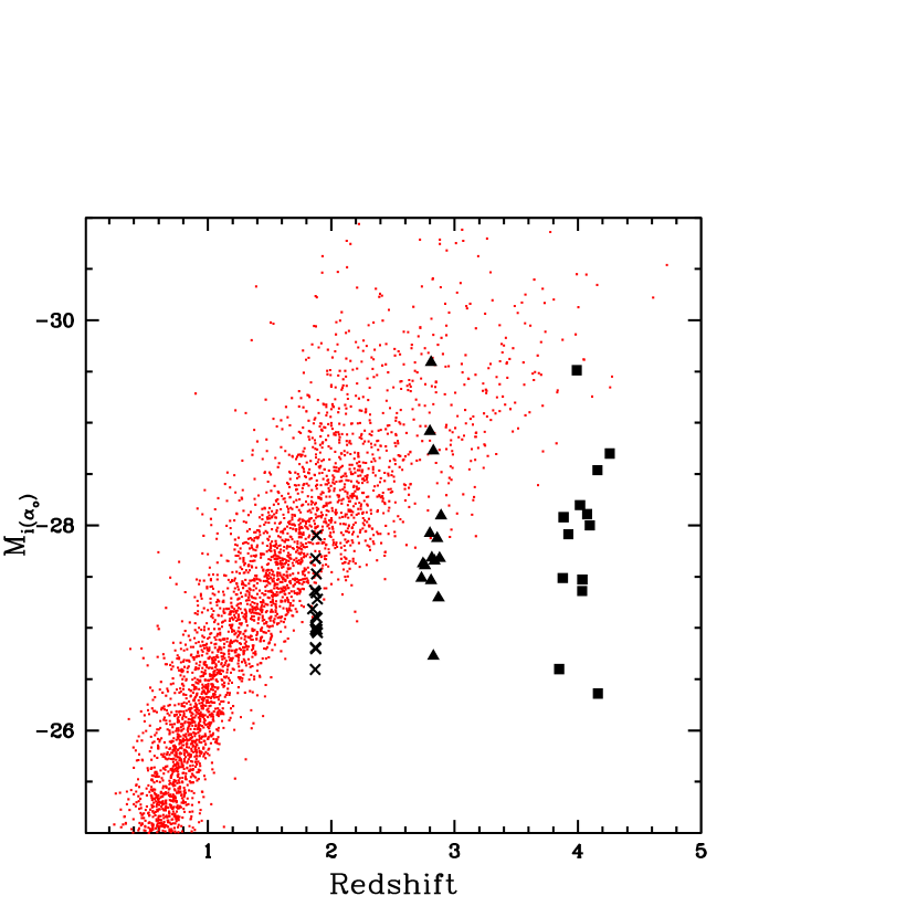
Figure 5: Absolute magnitude $M_{i(\alpha_{o})}$ vs. redshift for the SQIID sample (filled black symbols). Crosses represent quasars at $z\sim 1.88$, triangles at $z\sim 2.82$ and squares at $z\sim 4.03$. The red dots respresent SDSS quasars with 2MASS detections.

Figure 6: a) Spectral index $\alpha_{o}$ vs. redshift for the SDSS subsample observed with SQIID (closed symbols.) Also shown is the mean $\alpha_{o}$ for each redshift bin (open circles) with the value given below. The line is a linear fit to the sample given by the relation given at upper left. The mean for the sample as a whole is $\langle\alpha_{o}\rangle=-0.55\pm 0.42$. b) Spectral index $\alpha_{o}$ vs. $M_{i(\alpha_{o})}$ for the SQIID sample. The quasars at $z\sim 1.88$, $2.82$, and $4.03$ are shown as crosses, triangles, and squares, respectively. The fit to the data as a function of $M_{i(\alpha_{o})}$ is given in the upper left and shown as a solid line.

Figure 7: (Top panels) Residuals in $\alpha_{o}$ of the linear expressions given in Equations 9 and 10. (Bottom panels) Two dimensional projections of the residuals in $\alpha_{o}$ of the expression given in Equation 11. The residuals average to $\sim 0$, but exhibit strong scatter, with residuals as large as $\sim 1$ in all cases.

Figure 8: Left: (top) The distribution of restframe optical spectral indices, $\alpha_{o}$, for the SDSS quasars detected by 2MASS. The mean of the sample is $\langle\alpha\rangle=-0.70\pm 0.53$ and the median is $-0.57$. (bottom) The distribution of $\alpha_{o}$ for the SQIID sample. The mean of the sample is $\langle\alpha\rangle=-0.55\pm 0.42$ and the median is $-0.47$. Right: The distribution of $\alpha_{o}$ for the SQIID sample in each redshift bin. See Table 3 for sample statistics.

Figure 9: a) The difference in absolute magnitude, $M_{i}$, assuming $\alpha=-0.5$ and the $\alpha_{o}$ from Table 2, as a function of redshift, for the SQIID sample. Also given are the average difference in magnitude for each redshift interval. There is a trend with redshift reflecting the trend toward flatter contiuum slopes at higher redshifts for the sample, as demonstrated in Figure 6a. b) The same difference as a function of $M_{i}(\alpha_{o})$. The quasars at $z\sim 1.88$, $2.82$, and $4.03$ are shown as crosses, triangles, and squares, respectively.

Table 1: SQIID Sample Quasar Near-IR Photometry

SDSS DR3 designation	Redshift	$i^{*}$	$J$	$H$	$K_{s}$
SDSS 095048.48$-$000017.7	1.8802	19.562$\pm$0.024	17.778$\pm$0.121	16.909$\pm$0.153	16.513$\pm$0.089
SDSS 095938.28$-$003500.8	1.8753	18.593$\pm$0.018	17.728$\pm$0.100	17.374$\pm$0.210	16.630$\pm$0.085
SDSS 101119.94$-$004145.3	1.8879	19.098$\pm$0.020	17.676$\pm$0.064	17.831$\pm$0.201	16.323$\pm$0.058
SDSS 102517.58$+$003422.0	1.8879	18.091$\pm$0.014	17.011$\pm$0.051	16.787$\pm$0.083	16.134$\pm$0.051
SDSS 103204.74$-$001119.1	1.8715	18.690$\pm$0.021	17.915$\pm$0.089	17.563$\pm$0.156	17.052$\pm$0.111
SDSS 103427.57$-$002233.9	1.8698	19.153$\pm$0.024	18.366$\pm$0.128	18.089$\pm$0.302	17.659$\pm$0.214
SDSS 110725.70$+$003353.8	1.8732	18.581$\pm$0.018	17.896$\pm$0.103	17.071$\pm$0.147	16.434$\pm$0.102
SDSS 115115.38$+$003826.9	1.8805	17.593$\pm$0.016	16.869$\pm$0.047	16.423$\pm$0.091	15.617$\pm$0.066
SDSS 121655.39$+$001415.3	1.8706	18.233$\pm$0.014	17.570$\pm$0.061	17.079$\pm$0.127	16.581$\pm$0.075
SDSS 123505.91$-$003022.3	1.8804	18.584$\pm$0.016	17.062$\pm$0.048	17.144$\pm$0.115	16.120$\pm$0.079
SDSS 123514.94$+$004740.7	1.8747	19.000$\pm$0.018	18.199$\pm$0.087	17.755$\pm$0.159	17.684$\pm$0.115
SDSS 123947.61$+$002516.2	1.8483	19.585$\pm$0.035	18.326$\pm$0.147	17.770$\pm$0.213	16.934$\pm$0.142
SDSS 132742.92$+$003532.6	1.8736	18.337$\pm$0.016	17.155$\pm$0.049	16.778$\pm$0.089	15.986$\pm$0.071
SDSS 135605.41$-$010024.4	1.8860	18.812$\pm$0.015	17.722$\pm$0.063	17.504$\pm$0.111	16.720$\pm$0.051
SDSS 141015.36$-$001418.9	1.8758	18.673$\pm$0.017	17.743$\pm$0.087	17.055$\pm$0.133	16.379$\pm$0.074
SDSS 143641.24$+$001558.9	1.8659	18.401$\pm$0.015	17.347$\pm$0.114	17.055$\pm$0.109	15.839$\pm$0.110
SDSS 145838.04$+$002417.9	1.8847	18.520$\pm$0.015	17.602$\pm$0.069	17.309$\pm$0.142	17.086$\pm$0.110
SDSS 094745.26$-$004113.2	2.8287	18.922$\pm$0.017	17.480$\pm$0.124	16.883$\pm$0.202	16.270$\pm$0.109
SDSS 100423.27$-$004042.9	2.7320	18.627$\pm$0.014	17.637$\pm$0.067	17.245$\pm$0.142	16.869$\pm$0.103
SDSS 102832.09$-$004607.0	2.8592	17.839$\pm$0.017	16.986$\pm$0.041	16.842$\pm$0.109	16.560$\pm$0.068
SDSS 105808.47$+$003930.5	2.8149	18.392$\pm$0.023	17.568$\pm$0.065	17.161$\pm$0.145	16.342$\pm$0.073
SDSS 121323.94$+$010414.7	2.8292	20.185$\pm$0.038	19.229$\pm$0.203	17.910$\pm$0.245	18.329$\pm$0.345
SDSS 121920.26$+$010736.1	2.8005	19.453$\pm$0.022	18.047$\pm$0.083	17.323$\pm$0.128	17.137$\pm$0.116
SDSS 121933.25$+$003226.4	2.8791	19.342$\pm$0.030	18.023$\pm$0.079	17.394$\pm$0.104	16.611$\pm$0.095
SDSS 122730.37$-$010446.1	2.8701	18.798$\pm$0.026	17.780$\pm$0.063	17.554$\pm$0.114	16.954$\pm$0.105
SDSS 124551.44$+$010505.0	2.8088	17.896$\pm$0.014	16.397$\pm$0.252	15.368$\pm$0.153	15.321$\pm$0.184
SDSS 125241.55$-$002040.6	2.8909	18.520$\pm$0.013	17.320$\pm$0.150	17.023$\pm$0.129	16.492$\pm$0.171
SDSS 131128.35$+$004929.7	2.8090	18.726$\pm$0.015	17.395$\pm$0.059	17.408$\pm$0.120	16.757$\pm$0.062
SDSS 133647.14$-$004857.1	2.7997	17.413$\pm$0.020	16.091$\pm$0.049	15.600$\pm$0.064	15.360$\pm$0.047
SDSS 143307.40$+$003319.0	2.7432	19.176$\pm$0.022	17.571$\pm$0.082	16.877$\pm$0.131	16.587$\pm$0.094
SDSS 145754.03$+$003639.0	2.7603	18.820$\pm$0.019	17.810$\pm$0.092	17.027$\pm$0.134	16.840$\pm$0.105
SDSS 150611.23$+$001823.6	2.8377	18.832$\pm$0.016	17.466$\pm$0.053	17.145$\pm$0.119	17.209$\pm$0.121
SDSS 094822.96$+$005554.4	3.8777	20.083$\pm$0.037	18.605$\pm$0.183	18.203$\pm$0.362	17.559$\pm$0.150
SDSS 104837.40$-$002813.6	3.9918	19.094$\pm$0.068	16.219$\pm$0.030	15.672$\pm$0.049	15.265$\pm$0.033
SDSS 105254.59$-$000625.8	4.1619	19.535$\pm$0.024	18.823$\pm$0.153	18.824$\pm$0.643	18.255$\pm$0.309
SDSS 105602.37$+$003222.0	4.0361	19.411$\pm$0.028	18.409$\pm$0.176	18.160$\pm$0.324	17.349$\pm$0.140
SDSS 105902.73$+$010404.0	4.0978	19.208$\pm$0.021	18.122$\pm$0.123	17.541$\pm$0.200	16.984$\pm$0.108
SDSS 110813.85$-$005944.5	4.0175	19.254$\pm$0.020	18.523$\pm$0.091	17.571$\pm$0.126	16.717$\pm$0.077
SDSS 111224.18$+$004630.3	4.0346	19.647$\pm$0.026	18.667$\pm$0.170	18.184$\pm$0.361	17.519$\pm$0.160
SDSS 120138.56$+$010336.2	3.8475	19.867$\pm$0.028	18.723$\pm$0.172	18.781$\pm$0.491	18.291$\pm$0.263
SDSS 121531.55$-$004900.4	3.8842	19.863$\pm$0.037	18.660$\pm$0.150	17.975$\pm$0.219	17.058$\pm$0.107
SDSS 122600.68$+$005923.6	4.2586	18.859$\pm$0.021	17.836$\pm$0.064	17.044$\pm$0.111	16.490$\pm$0.073
SDSS 131052.50$-$005533.2	4.1585	18.847$\pm$0.023	17.650$\pm$0.129	17.193$\pm$0.225	16.569$\pm$0.084
SDSS 135828.74$+$005811.3	3.9225	19.318$\pm$0.022	18.048$\pm$0.079	17.368$\pm$0.132	17.240$\pm$0.096
SDSS 141315.36$+$000032.3	4.0760	19.700$\pm$0.027	18.352$\pm$0.092	17.562$\pm$0.186	17.188$\pm$0.106

Note. — Table 1 Optical $i^{*}$ photometry and redshift data are taken from the SDSS DR3Q (Schneider et al., 2005).

Table 2: SQIID Sample Spectral Indices

SDSS DR3 designation	Redshift	$A_{u}$	$M_{i(z=0)}$	$M_{i(z=2)}$	$\alpha_{o}$	$\sigma_{\alpha_{o}}$	$M_{i(\alpha_{o})}$
SDSS 095048.48$-$000017.7	1.8802	0.298	-25.777	-26.068	-1.77	0.12	-27.527
SDSS 095938.28$-$003500.8	1.8753	0.183	-26.694	-26.983	-0.34	0.09	-26.798
SDSS 101119.94$-$004145.3	1.8879	0.234	-26.225	-26.519	-0.88	0.07	-26.952
SDSS 102517.58$+$003422.0	1.8879	0.257	-27.241	-27.535	-0.28	0.05	-27.281
SDSS 103204.74$-$001119.1	1.8715	0.330	-26.651	-26.940	-0.39	0.07	-26.808
SDSS 103427.57$-$002233.9	1.8698	0.375	-26.205	-26.493	-0.59	0.10	-26.596
SDSS 110725.70$+$003353.8	1.8732	0.181	-26.702	-26.990	-0.61	0.07	-27.111
SDSS 115115.38$+$003826.9	1.8805	0.114	-27.672	-27.963	-0.45	0.04	-27.902
SDSS 121655.39$+$001415.3	1.8706	0.130	-27.026	-27.315	-0.21	0.06	-26.985
SDSS 123505.91$-$003022.3	1.8804	0.121	-26.684	-26.975	-0.49	0.05	-26.967
SDSS 123514.94$+$004740.7	1.8747	0.126	-26.263	-26.552	-0.90	0.08	-27.007
SDSS 123947.60$+$002516.2	1.8483	0.087	-25.629	-25.912	-1.62	0.14	-27.185
SDSS 132742.92$+$003532.6	1.8736	0.134	-26.928	-27.216	-0.90	0.05	-27.677
SDSS 135605.41$-$010024.4	1.8860	0.264	-26.521	-26.815	-0.75	0.06	-27.098
SDSS 141015.36$-$001418.9	1.8758	0.222	-26.630	-26.920	-0.87	0.07	-27.343
SDSS 143641.24$+$001558.9	1.8659	0.208	-26.884	-27.171	-0.67	0.06	-27.365
SDSS 145838.04$+$002417.9	1.8847	0.251	-26.806	-27.098	-0.40	0.06	-26.987
SDSS 094745.26$-$004113.2	2.8287	0.416	-27.390	-27.807	-1.13	0.09	-28.725
SDSS 100423.27$-$004042.9	2.7320	0.281	-27.553	-27.974	-0.16	0.07	-27.486
SDSS 102832.09$-$004607.0	2.8592	0.276	-28.440	-28.859	0.17	0.06	-27.874
SDSS 105808.47$+$003930.5	2.8149	0.216	-27.828	-28.245	-0.11	0.06	-27.682
SDSS 121323.94$+$010414.7	2.8292	0.171	-26.028	-26.445	-0.69	0.17	-26.727
SDSS 121920.26$+$010736.1	2.8005	0.102	-26.710	-27.126	-1.05	0.11	-27.923
SDSS 121933.25$+$003226.4	2.8791	0.130	-26.893	-27.314	-0.75	0.09	-27.681
SDSS 122730.37$-$010446.1	2.8701	0.121	-27.427	-27.846	-0.12	0.09	-27.293
SDSS 124551.44$+$010505.0	2.8088	0.103	-28.274	-28.690	-1.12	0.07	-29.591
SDSS 125241.55$-$002040.6	2.8909	0.159	-27.736	-28.158	-0.46	0.08	-28.093
SDSS 131128.35$+$004929.7	2.8090	0.161	-27.467	-27.883	-0.21	0.06	-27.464
SDSS 133647.14$-$004857.1	2.7997	0.140	-28.764	-29.181	-0.32	0.04	-28.918
SDSS 143307.40$+$003319.0	2.7432	0.186	-26.975	-27.393	-0.66	0.08	-27.628
SDSS 145754.03$+$003639.0	2.7603	0.266	-27.377	-27.794	-0.37	0.08	-27.610
SDSS 150611.23$+$001823.6	2.8377	0.309	-27.444	-27.861	-0.36	0.08	-27.654
SDSS 094822.96$+$005554.4	3.8777	0.562	-26.977	-27.445	-0.53	0.22	-27.488
SDSS 104837.40$-$002813.6	3.9918	0.208	-27.885	-28.361	-1.16	0.06	-29.513
SDSS 105254.59$-$000625.8	4.1619	0.254	-27.552	-28.056	0.45	0.18	-26.360
SDSS 105602.37$+$003222.0	4.0361	0.212	-27.593	-28.073	-0.16	0.17	-27.473
SDSS 105902.73$+$010404.0	4.0978	0.157	-27.806	-28.298	-0.33	0.13	-27.999
SDSS 110813.85$-$005944.5	4.0175	0.243	-27.753	-28.230	-0.48	0.10	-28.197
SDSS 111224.18$+$004630.3	4.0346	0.186	-27.346	-27.825	-0.24	0.16	-27.360
SDSS 120138.56$+$010336.2	3.8475	0.111	-26.993	-27.454	-0.00	0.19	-26.600
SDSS 121531.55$-$004900.4	3.8842	0.096	-27.012	-27.480	-0.85	0.15	-28.080
SDSS 122600.68$+$005923.6	4.2586	0.123	-28.223	-28.757	-0.47	0.11	-28.701
SDSS 131052.50$-$005533.2	4.1585	0.131	-28.188	-28.692	-0.41	0.11	-28.539
SDSS 135828.74$+$005811.3	3.9225	0.190	-27.616	-28.095	-0.40	0.10	-27.913
SDSS 141315.36$+$000032.3	4.0760	0.219	-27.328	-27.816	-0.67	0.14	-28.110

Note. — Table 2 Redshift and galactic extinction data are taken from the SDSS DR3Q (Schneider et al., 2005).

Table 3: Sample Spectral Index Statistics

					$\alpha_{o}$
Quasar Sample	N	$\langle z\rangle$	$\langle M_{i(\alpha_{o})}\rangle$	median	mean	$\sigma$
SDSS w/SQIID	45	2.81	-27.61	-0.47	-0.55	0.42
“J” subsample	17	1.88	-27.15	-0.61	-0.71	0.43
“H” subsample	15	2.82	-27.89	-0.37	-0.49	0.40
“K” subsample	13	4.03	-27.87	-0.41	-0.40	0.39
SDSS w/2MASS	6192	0.98	-25.62	-0.57	-0.70	0.53
SDSS w/2MASS ($-28<M_{i}<-26.5$)	1336	1.44	-27.29	-0.47	-0.54	0.37

References

- Babu & Feigelson (1996) Babu, G.J. & Feigelson, E.D. 1996, Astrostatistics: Interdisciplinary Statistics (1st Edition, London: Chapman & Hall)
- Bonnarel et al. (2000) Bonnarel, F., Fernique, P., Bienaymé, O., Egret, D., Genova, F., Louys, M., Ochsenbein, F., Wenger, M., & Bartlett, J.G. 2000, A&AS, 143, 33
- Boyle et al. (1987) Boyle, B.J., Fong, R., Shanks, T., & Peterson, B.A. 1987, MNRAS, 227, 717
- Buckley & James (1979) Buckley, J., & James, I. 1979, Biometrika, 66, 429
- Cristiani & Vio (1990) Cristiani, S. & Vio, R. 1990, A&A, 227, 385
- Croom et al. (2004) Croom, S.M., Smith, R.J., Boyle, B.J., Shanks, T., Miller, L., Outram, P.J., & Loaring, N.S. 2004, MNRAS, 349, 1397
- Cutri et al. (2003) Cutri, R.M. et al. 2003, The IRSA 2MASS All-Sky Point Source Catalog, http://irsa.ipac.caltech.edu/applications/Gator/
- Dempster et al. (1977) Dempster, A.P., Laird, N.M., & Rubin, D.B. 1977, Royal Stat. Soc. B, 39, 1
- Francis (1996) Francis, P.J. 1996, Publ. Astron. Soc. Aust., 13, 212
- Giallongo & Vagnetti (1992) Giallongo, E. & Vagnetti, F. 1992, ApJ, 396, 411
- Glikman et al. (2006) Glikman, E., Helfand, D.J. & White, R.L. 2006, ApJ, 640, 579
- Hogg (2000) Hogg, D.W. 2000, preprint (astro-ph/9905116)
- Hogg et al. (2002) Hogg, D.W., Baldry, I.K., Blanton, M.R., & Eisenstein, D.J. 2002, preprint (astro-ph/0210394)
- Holberg & Bergeron (2006) Holberg, J.B. & Bergeron, P. 2006, AJ, 132, 1221
- Hopkins et al. (2007) Hopkins, P.F., Richards, G.T., & Hernquist, L. 2007, ApJ, 654, 731
- Humason, Mayall, & Sandage (1956) Humason, M.L., Mayall, N.U., & Sandage, A.R. 1956, AJ, 61, 97
- Kelly et al. (2007) Kelly, B.C., Bechtold, J., Siemiginowska, A., Aldcroft, T., & Sobolewska, M. 2007, ApJ, 657, 116
- Kennefick et al. (1995) Kennefick, J.D., Djorgovski, S.G., & de Carvalho, R.R. 1995, AJ, 110, 2553
- Kennefick et al. (1997) Kennefick, J.D., Osmer, P.S., Pahre, M. & Djorgovski, S. 1997, in N.R. Tanvir, A. Aragon-Salamanca and J.V. Wall (eds.), The Hubble Space Telescope and the High Redshift Universe, Singapore: World Scientific Publishing Company, p. 401
- Koratkar & Blaes (1999) Koratkar, A.,, & Blaes, O. 1999, PASP, 111, 1
- La Franca & Cristiani (1997) La Franca, F. & Cristiani, S. 1997, AJ, 113, 1517
- LaValley et al. (1992) LaValley, M., Isobe, T., & Feigelson, E. 1992, A.S.P. Conference Series, 25, 245
- Mégessier (1995) Mégessier, C. 1995, A&A, 296, 771
- Oke & Gunn (1983) Oke, J.B. & Gunn, J.E. 1983, ApJ, 266, 713
- Oke & Sandage (1968) Oke, J.B. & Sandage, A. 1968, ApJ, 154, 21
- Pentericci et al. (2003) Pentericci, L., Rix, H.W., Prada, F., Fan, X., Strauss, M.A., Schneider, D.P., Grebel, E.K., Harbeck, D., Brinkmann, J., & Narayanan, V.K. 2003, A&A, 410, 75
- Press et al. (1992) Press, W.H, Teukolsky, S.A., Vetterling, W.T., & Flannery, B.P. 1992, Numerical Recipes in Fortran: The Art of Scientific Computing (2nd Edition, Cambridge: Cambridge University Press)
- Richards et al. (2006a) Richards, G.T. et al. 2006, AJ, 131, 2766
- Richards et al. (2006b) Richards, G.T. et al. 2006, ApJS, 166, 470
- Richards et al. (2003) Richards, G.T. et al. 2003, AJ, 126, 1131
- Schlegel et al. (1998) Schlegel, D.J., Finkbeiner, D.P., & Davis, M. 1998, ApJ, 500, 525
- Schmidt & Green (1983) Schmidt, M. & Green, R.F. 1983, ApJ, 269, 352
- Schmidt, Schneider & Gunn (1995) Schmidt, M., Schneider, D.P., & Gunn, J.E. 1995, AJ, 110, 68
- Schneider et al. (2002) Schneider, D.P. et al. 2002, AJ, 123, 567
- Schneider et al. (2005) Schneider, D.P. et al. 2005, AJ, 130, 367
- Schneider et al. (2007) Schneider, D.P. et al. 2007, AJ, 134, 102
- Spergel et al. (2007) Spergel, D.N. et al. 2007, ApJS, 170, 377
- Steffen et al. (2006) Steffen, A.T., Strateva, I., Brandt, W.N., Alexander, D.M., Koekemoer, A.M., Lehmer, B.D., Schneider, D.P., & Vignali, C. 2006, 131, 2826
- Tang et al. (2007) Tang, S.M., Shuang, N.Z., and & Hopkins, P.F. 2007, MNRAS, 377, 1113
- Vanden Berk et al. (2001) Vanden Berk, D.E. et al. 2001, AJ, 122, 549
- Warren, Hewett & Osmer (1994) Warren, S.J., Hewett, P.C., & Osmer, P.S. 1994, ApJ, 421, 412
- Webster et al. (1995) Webster, R.L., Francis, P.J., Peterson, B.A., Drinkwater, M.J., & Masci, F.J. 1995, Nature, 375, 469
- Wisotzki (1998) Wisotzki, L. 1998, Astron. Nachr., 319, 257
- Wisotzki (2000) Wisotzki, L. 2000, A&A, 353, 861