Single fiber transport by a fluid flow in a fracture with rough walls: influence of the fluid rheology

Abstract

The possible transport of fibers by fluid flow in fractures is investigated experimentally in transparent models using flexible polyester thread (mean diameter $280\mu\mathrm{m}$) and Newtonian and shear thinning fluids. In the case of smooth parallel walls, fibers of finite length $\ell=20-150\,\mathrm{mm}$ move at a constant velocity of the order of the maximum fluid velocity in the aperture. In contrast, for fibers lying initially at the inlet side of the model and dragged by the flow inside it, the velocity increases with the depth of penetration (this results from the lower velocity - and drag - in the inlet part). In both cases, the friction of the fiber with the smooth walls is weak. For rough self-affine walls and a continuous gradient of the local mean aperture transverse to the flow, transport of the fibers by a water flow is only possible in the region of larger aperture ($\bar{a}\gtrsim 1.1\mathrm{mm}$) and is of “stop and go” type at low velocities. Time dependent distorsions of the fiber are also often observed. When water is replaced by a shear thinning polymer solution, the fibers move faster and continuously in high aperture regions and their friction with the walls is reduced. Fiber transport becomes also possible in narrower regions where irreversible pinning occurred for water. In a third rough model with no global aperture gradient but with rough walls and a channelization parallel to the mean flow, fiber transport was only possible in shear-thinning flows and pinning and entanglement effects were studied.

I Introduction

Fiber transport by flowing fluids is of interest in many areas of physics, biology and engineering: examples include the transport of paper pulp Stockie and Green (1998), the manufacturing of fiber-reinforced composites Yasuda et al. (2002), the rheology of biological polymers Lagomarsino et al. (2005) and the motility of micro-organisms Lowe (2003); Purcell (1977). Recently, also, using long optical fibers has been suggested as a method to realize distributed in-situ measurements (temperature for instance) on natural water flows Selker et al (2006): this raises the problem of the possible transport of the fiber by the moving fluid which often occurs in geometries confined by solid walls. More precisely, little work has been devoted to flow channels with rough walls such as fractures of natural rocks and of materials of industrial interest in civil, environmental and petroleum engineering. In that case, the interactions of the fibers with the walls are particularly important and may lead to blockage of the motion of the fibers and/or to clogging of the channels. In addition to their practical applications, these processes raise fundamental questions regarding the motion of flexible solid bodies in complex flow fields.

The objective of the present experimental study is to understand the transport of fibers by the flow and to investigate the role of the flow geometry and fluid rheology. Here, single fractures are modeled by the space (saturated by a flowing fluid) between either two parallel plane walls or two complementary rough self-affine walls with a relative shear displacement from their contact position. This latter configuration allows one to reproduce preferential flow channels on Fracture Characterization and Flow (1996); Adler and Thovert (1999) which are a widespread feature of natural fractures and influence strongly their transport properties. The walls of the fracture are transparent to allow for optical observations of the motion of the fibers.

In addition to hydrodynamic forces on the fibers due to the relative velocity with the fluid, their motion and deformation is influenced by different effects. A first one is the interaction forces with the walls: they are particularly important when the diameter of the fibers is comparable to the local channel aperture or when they are close to one of the walls Sugihara-Seki (1993); Petrich and Koch (1998). Second, tension forces reflecting the mechanical cohesion of the fiber are present all along its length so that the motion of each region influences the other ones. Tension and hydrodynamic forces add-up and their spatial variations in shear flows or flows with curved streamlines deform the fibers (although their length remains constant): this may finally lead to entanglement and blockage. Next, these deformations are opposed by elastic forces reflecting the non-zero stiffness of the fibers: their relative magnitude with respect to the hydrodynamic forces is a particularly important parameter of the problem Forgacs and Mason (1959a). On the one hand, very flexible fibers would seem to be able to follow the streamlines but, on the other hand, loops may appear easily and lead to trapping in narrow zones Forgacs and Mason (1959b). Another key element is the rheology of the fluids which influences strongly the hydrodynamic forces on slender bodies, even in simple shear flows Leal (1975). Finally, inertia (particularly in regions of large spatial flow velocity variations) and gravity may also be of importance by inducing motions transverse to the flow and towards the walls.

In the following, the feasibility of fiber transport and its dependence on the mechanisms discussed above are studied in three different model fractures. A first one has smooth walls and is used as a reference case and the two others have rough walls with self affine geometries. For one of the rough fractures ($F3$), the mean planes of the walls are parallel. For the other one ($F2$), they have a small angle resulting in a non-zero transverse gradient of the mean aperture: this wedge shape mimicks the edge of many natural fractures. In this work, the influence of the geometry of the fibers on their transport is analyzed by comparing the motion of finite length segments (still with an aspect ratio greater than $200$) and of continuous threads injected at the inlet of the fracture. The influence of deformations due to flow velocity gradients could be investigated by using flexible thin fibers made of polyester thread. Special attention has been brought to the mechanisms of pinning during the motion of the fibers and of possible depinning after enough elastic energy has been accumulated (see sections III.2 and IV.1). Finally, the influence of the fluid rheology has been studied by comparing fiber transport by Newtonian and shear thinning fluids.

II Experimental set-up and procedure

II.1 Fiber characteristics

The experimental fibers are prepared from commercial polyester thread used for needlework and made of two strands twisted together. The section is not circular so that the diameter varies between $220$ and $340\ \mu m$. The specific mass of the fiber is $\rho=1.8\pm 0.1\times 10^{-3}\,kg/m^{3}$. Its bending stiffness $EI$ (ratio of the applied bending momentum by the curvature) is of the order of $10^{-9}\,kg.m^{3}/s^{2}$ (a value similar to that reported in ref. Habibi et al. (2007) for a comparable material). This value has been estimated by measuring the deflection under its own weight of a horizontal fiber segment attached at one end Landau and Lifshitz (1986).

The choice of these multifilament fibers reflects a trade-off between several requirements. The fiber diameter is large enough to be clearly visible and its flexibility is both high enough to allow for deformations by the fluid velocity gradients and low enough so that coils do not build up too easily (see introduction). We verified indeed that monofilament wires of similar (and even smaller) diameters were too rigid and retain often, in addition, a permanent curvature.

Both segments of fiber and continuous fibers were used in the present work. The segments are cut out of polyester thread with a length $20\,\mathrm{mm}\leq\ell\leq 150\,\mathrm{mm}$. The continuous fibers are also cut out of a spooled thread but with a length larger than that of the fracture: they are progressively injected from above into the fracture under zero applied tension conditions. A specific procedure is used to avoid blunting the ends of the fibers and the fibers are carefully saturated with liquid prior to the experiments.

II.2 Model fractures

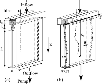
Figure 1: Schematic view of the experimental models. (a) fracture with flat parallel walls - (b) fracture with complementary self-affine walls with a relative displacement $\vec{u}$. For all cells : $w=90\ \mathrm{mm}$, $a_{b}=20\ \mathrm{mm}$, $a_{e}=5\ \mathrm{mm}$, $l_{e}=52\ \mathrm{mm}$, $l_{b}\sim 20\ \mathrm{mm}$ and $L=288\ \mathrm{mm}$. The mean flow is vertical and parallel to $x$

The fracture models are manufactured with the same technique as in Ref. Boschan et al. (2007) by carving two parallelepipedic plexiglas blocks using a computer controlled milling machine. The two blocks are then clamped together in a preset position determined by the geometry of the sides of the block: these act as spacers leaving a controlled interval between the surfaces for the fluid flow (Fig. 1). This procedure allows for the realization of model fractures with rough (or smooth) walls of arbitrary geometries and three of them have been used.

The first sample (refered to as $F1$) has smooth parallel plane walls separated by a fixed distance $a(x,y)=0.65\ \mathrm{mm}$ (Fig. 1a). The two other models have complementary rough walls with a self affine geometry of characteristic Hurst exponent $H=0.8$: this value is similar to that measured on granite fractures Boffa et al. (1998) and in various other materials Bouchaud (2003). The amplitude of the roughness, represented by the difference between the heights at the highest and lowest points of the surface is equal to $26\ \mathrm{mm}$: this corresponds also to values measured on natural rock fractures Poon et al. (1992). For these two models, the wall surfaces are perfectly complementary: in order to generate aperture fluctuations, they are positioned with a small relative shear displacement $\vec{u}=0.65\ \mathrm{mm}$ in the direction $y$ normal to the flow (Fig. 1b).

The resulting aperture maps are displayed for the two models in Figures 4 and 10 using a color code. The bottom curves represents the transverse profile in the $y$ direction of the average along $x$ of the aperture. In model $F2$, there is a small angle between the mean plane of the surfaces mimicking the edge of natural fractures. As a result, the average $\overline{a}$ of the aperture along the direction $x$ of the flow decreases with the coordinate $y$ from $\overline{a(y=0)}=1.1\ \mathrm{mm}$ to $\overline{a(y=w)}=0.8\ \mathrm{mm}$ with a global mean value $\bar{a}=0.91\ \mathrm{mm}$ (Fig. 4c); $w$ is the width of the cell and $y=0$ and $y=w$ correspond to the sides of the experimental region. Note that the wedge shape of the model results in a global color gradient in the direction $y$ in the maps of Fig. 4a-b. The root mean square amplitude $\sigma_{a}(y)=(<(\overline{a(y)}-a(x,y))^{2}>_{x})^{1/2}$ of the fluctuations of the aperture in the direction $x$ with respect to the mean value $\overline{a(y)}=<a(x,y)>_{x}$ is equal to $\sigma_{a}(y)=0.122\ \mathrm{mm}$ and independent of $y$. Therefore, the fluctuations remain of constant absolute amplitude while the mean aperture varies with $y$.

In model $F3$, the mean planes of the fracture walls are parallel with a distance $a=0.65\ \mathrm{mm}$ comparable to the value for model $F1$. The local fluctuations of the aperture are of the same order of magnitude as the deviations from the linear trend in model $F2$ (Fig. 10c). No global trend in the color shade at the scale of the global size of the fracture is visible in the map of Fig. 10a-b. Comparing experiments realized with the two systems allows one to discriminate between the influence of the roughness and that of the global transverse aperture gradient.

II.3 Experimental set-up and procedure

The model fractures are held vertically; liquid is sucked uniformly at the bottom side at a constant flow rate and reinjected at the top into an open bath of area $5\times 100\ \mathrm{mm}$ and depth $l_{b}\sim 10\,\mathrm{mm}$ covering the inlet of the model. This design allows one to introduce the fibers in the bath through its open surface and then into the fracture. In order to make the injection of the fibers easier, the upper section has a funnel-like “Y” shape, i.e. the mean aperture of the fracture increases with height in the top $52\,\mathrm{mm}$ of the model (distance $l_{e}$ in Figs. 1a-b).

The model is illuminated from behind by a light panel and a digital camera provides images with $1024\times 768$ pixels at a rate of $30$ frames per second and with an exposure time of $1/300\ \mathrm{s}$. The length of the field of view is $150\ \mathrm{mm}$ in the vertical direction parallel to the flow and the top of the aperture maps corresponds to a distance of $110\ \mathrm{mm}$ from the inlet of the fracture.

On each picture, the location and geometry of the fiber is determined by a binary thresholding technique. For most experiments, except in some cases in which the fiber gets pinned, its distortions are moderate and it remains overall aligned with the direction of the flow. Therefore, at each distance $x$ from the inlet, there is only one point along the fiber centerline, and, therefore, only one value of $y$. ¿From these data, spatiotemporal-diagrams like those displayed in Figs. 3a-b are obtained. The vertical scale corresponds to the vertical distance $x$, the horizontal one to time and the color code corresponds to the distance $y$ at the corresponding value of $x$. Qualitatively, these diagrams provide information on the global motion of the fibers, on their rotation and on their deformation. For instance, diagrams with uniform colors on horizontal lines correspond to a pure translation of the fiber in the direction parallel to the mean flow; in contrast, color variations of these lines imply lateral motions. Quantitatively, the velocity of segments of fibers with a finite length is take equal the variation between two successive images of the vertical distance $x_{m}$ of their center of mass to the inlet side of the model. For continuous fibers, one uses instead the variation of the distance $x_{t}$ of the tip of the fiber to the inlet. In both cases, the vertical velocity component of the center of mass (respectively tip) of the fiber will be referred to as $V_{f}$. Continuous fibers are more easily retrieved after the experiments than fiber segments when trapping occurs: for that reason, most experiments in rough fractures have been realized with continuous fibers in order to obtain more data.

II.4 Characteristics of the fluids

The Newtonian fluid used in the experiments is high purity water (Millipore - Milli-Q grade) with a specific mass $\rho=10^{3}\ \mathrm{kg/m^{3}}$ and a dynamic viscosity $\mu_{\infty}\simeq 1\ \mathrm{mPa.s}$. The shear thinning fluid is a solution of high molecular weight Scleroglucan (Sanofi Bioindustries) in water at a concentration $C_{p}=1000\ \mathrm{ppm}$. The variation of the effective viscosity $\mu$ with the shear rate $\dot{\gamma}$ (see Figure 2 of ref. D’Angelo et al. (2007)) is well described by the Carreau function:

$$\mu=\frac{1}{(1+(\dot{\gamma}/\dot{\gamma_{0}})^{2})^{\frac{1-n}{2}}}(\mu_{0}-\mu_{\infty})+\mu_{\infty}.$$ (1)

with $n=0.26$, $\dot{\gamma_{0}}=0.026\pm 0.004\ \mathrm{s^{-1}}$, ${\mu}_{0}=4500\pm 340\ \mathrm{mPa.s}$. A shear thinning domain of shear rates in which $\mu\propto{\dot{\gamma}}^{(n-1)}$ is bounded by two Newtonian domains. At low shear rates ($\dot{\gamma}\ll\dot{\gamma_{0}}$), the viscosity is constant with $\mu=\mu_{0}$. At very high shear rates ($\dot{\gamma}\gg\dot{\gamma}_{\infty}=\dot{\gamma_{0}}(\mu_{0}/\mu_{\infty})^{1/1-n}$), the effective viscosity should reach the limiting value $\mu_{\infty}$. Practically, and following theoretical expectations, $\mu_{\infty}$ is taken equal to the viscosity of the solvent (i.e. $\mu_{\infty}=1\ \mathrm{mPa.s}$ for water) because it cannot be measured directly (the corresponding transition shear rate $\dot{\gamma}_{\infty}\simeq 2300\ \mathrm{s^{-1}}$ is above the useful range of our rheological measurements ($\dot{\gamma}<100\ \mathrm{s^{-1}}$)).

II.5 Characteristic velocities and shear rates in the experiments

In the present experiments, the mean flow velocity ranges from $U=50$ to $400\ \mathrm{mm/s}$. For water, the corresponding Reynolds number defined as $Re=U\bar{a}\rho/\mu$ varies from $40$ and $320$: substantial inertial effects are therefore expected Zimmerman et al. (2004), and will be larger for rough fractures. An alternative value of the Reynolds number is obtained by using the diameter of the fiber and its relative velocity with respect to the fluid; it remains however higher than $1$, confirming the need to take into account inertial effects.

Regarding the shear rate $\dot{\gamma}$, it is equal to zero in the center part of the aperture and reaches a maximum $\dot{\gamma}_{w}$ at the walls. For a Newtonian fluid, $\dot{\gamma}_{w}=6U/a$ (neglecting the influence of the fiber and of the roughness of the walls). For shear thinning fluids Gabbanelli et al. (2005), $\dot{\gamma}_{w}$ depends on the relative values of the shear-rate $\dot{\gamma}$ and of the parameters $\dot{\gamma_{0}}$ and $\dot{\gamma}_{\infty}$ (see Sec. II.4) in the flow. At very low mean flow velocities $U$ for which $\dot{\gamma}_{w}\leq\dot{\gamma_{0}}$, the viscosity would be equal to $\mu_{0}$ in the full fluid volume and the results would be the same as for a Newtonian fluid. Using the numerical values from Sec. II.4, this would require that $U<a\dot{\gamma_{0}}/6=2.16\times 10^{-3}\,\mathrm{mm/s}$, a value well below the present experimental range ($U>50\,\mathrm{mm/s}$). The fluid has therefore a shear thinning behavior in a part of the flow volume.

In the opposite high velocity limit, a second Newtonian layer with $\mu=\mu_{\infty}$ develops at the walls if $\dot{\gamma}_{w}>\dot{\gamma}_{\infty}$. Assuming a truncated power law rheological curve (see Gabbanelli et al. (2005)), the corresponding threshold value of $U$ may be estimated as: $U=\dot{\gamma}_{\infty}a\left(\frac{1}{6}\right)^{1/n}\left[\frac{3n}{2n+1}\right]$. Using the numerical values from Sec. II.4, this leads to $U=2\,\mathrm{mm/s}$, again below the experimental range of velocities used in the present work. A second Newtonian layer of viscosity $\mu_{\infty}$ appears therefore on the walls in our experiments and the effective local viscosity increases from $\mu_{\infty}$ at the walls to $\mu_{0}$ in the center of the gap. The thickness $\delta z$ of the Newtonian layer of viscosity $\mu_{\infty}$ on the walls at the highest experimental flow velocity $U=400\,\mathrm{mm/s}$ may be estimated from the relation $2\delta z/a=1-a\dot{\gamma}_{\infty}/(6U)$ valid if $\dot{\gamma}_{w}\gg\dot{\gamma}_{\infty}$: the combined thicknesses of these two Newtonian layers on both walls are of the order of $52\%$ of the gap $a$.

III Fiber transport by water in smooth and rough model fractures

III.1 Fracture with smooth walls (model $F1$)

III.1.1 Transport of fiber segments

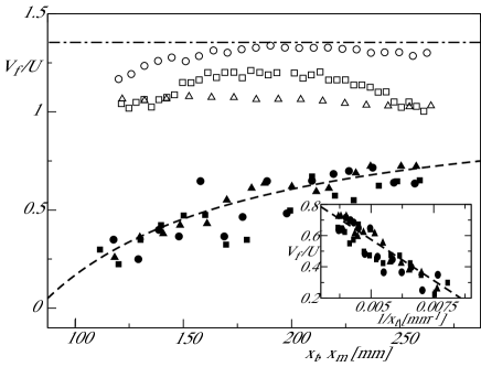
Figure 2: Variation of the normalized velocities $V_{f}/U$ of the tip of continuous fibers as a function of the distance $x_{t}$ of the tip from the injection side of the model: ($\blacksquare$) $U=\ 100\,\mathrm{mm/s}$, ($\bullet$) $U=\,150\ \mathrm{mm/s}$, ($\blacktriangle$) $U=\ 290\,\mathrm{mm/s}$. Variation of the velocity $dx_{m}/dt$ of the center of mass of fiber segments of length $\ell=20\mathrm{mm}$ as a function of $x_{m}$: ($\square$) $U=\,100\,\mathrm{mm/s}$, ($\circ$) $U=\,150\,\mathrm{mm/s}$, ($\triangle$) $U=\,290\,\mathrm{mm/s}$. Dashed line : $V_{f}/U=1.1-105/x_{t}$. Inset: variation of $V_{f}/U$ as a function of $1/x_{t}$ for the continuous fiber (same symbols as in main graph). Dash-dotted line: estimated value $V_{f}/U=1.35$ from ref. Sugihara-Seki (1993)

As a first step, reference experiments were carried out on the model fracture $F1$ with flat smooth walls, starting with fiber segments of length $\ell$ ranging from $20$ to $150\,\mathrm{mm}$ and at mean velocities $U$ of the fluid across the aperture: $50\leq U\leq 400\,\mathrm{mm/s}$. It should be noted, in addition, that few experimental and even numerical results (outside reference Sugihara-Seki (1993)) are available on the transport of fibers, even in the simple geometry of parallel plane walls). The present study is centered on the transport of fibers with their mean axis parallel on the average to the direction of the flow within $\pm 10^{\circ}$. For each set of values of $\ell$ and $U$, more than $20$ transport experiments were realized. In all cases, no deformation of the fibers is visible during the motion and they reach a velocity which is constant with the distance $x_{m}$ of their center of mass to the injection side within $\pm 10\%$. This latter result is visible in Figure 2 in which the ratio of the velocity of the fiber ($V_{f}$) and of the mean fluid velocity ($U$) is plotted as a function of $x_{m}$ for $3$ different $U$ values (open symbols) in a range of $1$ to $3$. Taking into account the intrinsic dispersion due to the injection process and the variability of the shape of the fiber, the variations of $V_{f}/U$ ($\leq 25\%$) are too small to suggest any definite dependence of $V_{f}/U$ on $U$. More generally, in other experiments performed at different velocities and for fibers of different lengths, $V_{f}/U$ always ranges between $1$ and $1.35$ at all values of $x_{m}$.

These observations can be compared to the numerical simulations by Sugihara-Seki Sugihara-Seki (1993) of the longitudinal velocity of a neutrally buoyant circular cylinder located midway between the walls of a plane channel. For a ratio of the diameter of the cylinder to the distance between the walls equal to $0.5$ as in the present experiments, the normalized predicted velocity $V_{c}/U$ is equal to 1.35 Sugihara-Seki (1993); this is consistent with the upper bound of the present experimental results (dash-dotted line in Fig. 2). The lower values would then correspond to cases in which the fiber is not in the center of the interval or in which it has a wavy shape which obstructs partly the flow field.

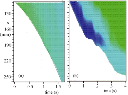
Figure 3: Spatiotemporal diagram of the transport of a continuous fiber by a downward flow of water in two model fractures. Horizontal axis: time - vertical axis: distances in the vertical direction counted from the top of the model (see Fig. 1). Color code: transverse coordinate $y(x)$ of fiber at the corresponding distance $x$. (a) Fracture $F1$ with smooth walls. ($U=120\,\mathrm{mm/s}$). $y$ ranges from $52.9\,\mathrm{mm}$ (green shade) to $63.3\,\mathrm{mm}$ (light blue) - (b) Fracture $F2$ with rough walls ($U=160\,\mathrm{mm/s}$). $y$ ranges from $58.4\,\mathrm{mm}$ (green) to $71.5\,\mathrm{mm}$ (dark blue). End of fiber inserted initially in the high permeability region of the fracture ($a>1\,\mathrm{mm}$).

III.1.2 Transport of continuous fibers

The above results are now compared to the case of a continuous fiber lying initially at the top of the model with no external force applied and dragged by the flowing fluid into the space between the fracture walls once its tip has been inserted into it. Figure 3a displays a spatiotemporal diagram obtained for such an experiment by the technique described in Sec. II.3. At a given time $t$, the color is constant along $x$ in the colored zone, indicating that the fiber remains straight and vertical. The color varies slightly with time which reflects a small global transverse displacement. The boundary of the colored zone marks the coordinate $x_{t}$ of the tip at the corresponding time $t$: its slope (proportional to the velocity $V_{f}$) increases with $t$. Quantitatively, Fig. 2 shows (dark symbols) that the normalized velocity $V_{f}/U$ of the tip of the fiber increases with $x_{t}$ ($U$ is the mean flow velocity in the constant aperture part of the model).

We show now by a simple model that this variation of $V_{f}/U$ reflects the lower flow velocity in the upper $52\,\mathrm{mm}$ of the fracture due to the larger cross section of the flow (this upper part has a “$Y$” shape with an aperture increasing towards the top). We assume that the fiber: a) remains straight and vertical so that the velocity of all its points is equal to $V_{f}$ and: b) is located in the center of the gap where the velocity has a maximum value $V_{M}(x)$ (assumed to be independent of the transverse coordinate $y$).

As a very first approximation, the local vertical viscous force $f_{v}$ per unit length on the fiber is taken equal to $f_{v}=\mu C(V_{M}(x)-V_{f})$ in which $C$ is a geometrical constant. Due to the low angle and the small distance between the walls for $x>0$, the flow field is quasi parallel with a Poiseuille-like profile between the walls at a given vertical coordinate $x>0$ (for a Newtonian fluid and neglecting flow perturbation by the fiber). In the upper fluid bath ($x<0$), this result is not satisfied but the fluid velocity is low enough so that its contribution is negligible.

In order to comply with volume flow rate conservation, the mean fluid velocity $\overline{V}(x)$ at the distance $x$ where the local aperture is $a(x)$ must satisfy: $\overline{V}(x)\,a(x)=Ua=cst(x)$ in which $a$ is the the aperture in the parallel part of the cell. where the mean velocity is $U$. The total viscous force on the continuous fiber between its lower tip at the vertical coordinate $x_{t}$ and the surface of the upper bath is then :

$$F_{v}(x_{t})=\int_{-l_{b}}^{x_{t}}f_{v}(x)dx=\mu C\left[BUa\int_{0}^{x_{t}}\frac{dx}{a(x)}-(l_{b}+x_{t})V_{f}\right]$$ (2)

$a(x)=a$ for $x\geq l_{e}$ and $a(x)$ decreases linearly from $a_{e}$ to $a$ with $x$ for $0\leq x\leq l_{e}$. As mentioned above, the velocity of the fluid in the upper bath ($x<0$) has been neglected. The coefficient $B$ would be equal to $3/2$ for a Poiseuille profile with no obstruction effect. The integral may be readily computed and $V_{f}$ may be estimated by taking $F_{v}=0$: this is equivalent to neglecting inertial forces as well as friction on the walls which has been found to be approximately valid in the case of the previous segments (the fiber moved roughly at the maximum velocity in the gap). This leads to:

$$V_{f}(x_{t}+l_{b})=BU\left[x_{t}-l_{e}+\frac{l_{e}a}{a_{e}-a}\ell n\frac{a_{e}}{a}\right]$$ (3)

The ratio $V_{f}/U$ may then be rewritten as:

$$\frac{V_{f}}{U}=b^{*}\left[1-\frac{l^{*}}{x_{t}+l_{b}}\right]$$ (4)

in which $b^{*}$ and $l^{*}$ are two constants and $x_{t}+l_{b}$ is the vertical distance of the tip of the fiber to the free surface of the bath. Using the parameter values given in Fig. 1 leads to the theoretical prediction: $b^{*}=B=3/2$ and $l^{*}=l_{b}+l_{e}(1-a\,\ell n(a_{e}/a)/(a_{e}-a))\simeq 57\,\mathrm{mm}$. Experimentally, $b^{*}$ and $l^{*}$ can be determined conveniently by plotting $V_{f}/U$ as function of $1/(x+l_{b})$ (inset of Fig. 2). The variation is linear as expected and a linear regression over the data gives the values $b^{*}=1.1\pm 0.1$ and $l^{*}=105\pm 15\,\mathrm{mm}$. These values are valid for all three velocities $U$ investigated and also lead, as might be expected, to a good fit (dotted line) in the main graph of of Fig. 2. The difference between the experimental and theoretical coefficients likely reflects perturbations of the flow profile by the fiber so that both $B$ and $C$ may differ from the theoretical value and depend on $x$. Finally, neglecting the influence of the inlet would only be possible for $x>>l^{*}$. This is not the case here since the global fracture length is only $\simeq 3l^{*}$.

III.2 Fiber transport in a wedged fracture with rough walls

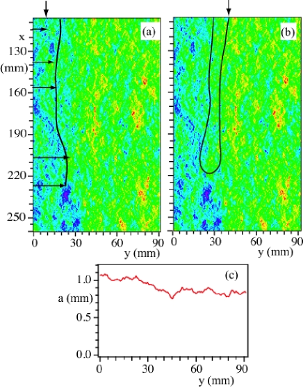
Figure 4: (a-b)Snapshots of continuous fibers (in black) during experiments realized in model $F2$ with two transverse injection distances (vertical arrows). The images of the fiber are superimposed onto a color coded map of the aperture field (red: $a\leq\,0.4\,\mathrm{mm}$, blue: $a\geq 1.4\,\mathrm{mm}$). Field of view: $90\times 150\,\mathrm{mm}$. Distances in the vertical $x$ direction are counted from the top of the model (see Fig. 1). Vertical arrows mark the location of the entry point of the fibers inside the field of view. a) $U=160\,\mathrm{mm/s}$; horizontal arrows: $5$ pinning positions b) $U=250\,\mathrm{mm/s}$. The fiber is pinned outside the image at a point of coordinates ($x\,=\,150\mathrm{mm}$ and $y\,=\,60\mathrm{mm}$). (c) variation of the aperture averaged along the distance $x$ parallel to the flow as a function of the transverse distance $y$.

While, for fractures with smooth plane walls, the fluid velocity is constant with $x$ and $y$ and no deformation of the fibers is observed, the flow field is very complex in rough fractures with large shear stresses in the fracture plane. If the fiber is sufficiently flexible, it may get bent by these stresses. Also, friction of the fibers with the walls is larger than for the smooth fracture of Sec. III.1 and it screens the influence of the inlet much more efficiently. All the experiments with rough walls described in the rest of the paper have been realized with a continuous fiber.

Fiber transport by a water flow has been studied in fracture $F2$ which has a self-affine roughness geometry with a small angle between the mean planes of the walls. In this model, one has both random variations of the velocity due to the roughness and a mean transverse gradient. Since the mean aperture ${\bar{a}}(y)$ varies continuously with $y$ (Fig. 4c), this allows us to test the minimum value of $\bar{a}(y)$ (averaged over the length $L$) for which fiber transport all along the fracture is possible. In the experiments using water as the carrier fluid, this minimum value was found to be of the order of $1\,\mathrm{mm}$ (typical mean aperture in the left side of the maps of Figs. 4). A view of a fiber obtained during such an experiment is superimposed onto the aperture field in Figure 4a. In the low aperture part, most fibers get pinned in the first cm past the initial large aperture section at the top of the model. However, in a few experiments performed at high flow rates ($U\geq 250\,\mathrm{mm/s}$), the tip of the fiber gets first pinned but a loop builds up downflow of the tip (Fig. 4b); then, the bottom of the loop moves sideways into the high aperture region where the velocity is largest. Finally, the loop pursues its downward motion until it reaches the bottom of the model.

Let us now concentrate on the dynamics of a fiber injected in the high permeability (large aperture) region at the left. Figure 3b displays a spatiotemporal diagram of such an experiment: it differs strongly from the diagram of Fig. 3a obtained for a model with plane walls. The motion of the tip is not continuous but corresponds to a sequence of “stop” and “go” phases marked respectively by horizontal and oblique sections of the boundary of the colored zone in Fig. 3b. The duration of individual pinning events may range from less than $1\ \mathrm{s}$ to nearly $10\ \mathrm{s}$ (about $10\ \%$ of the total transit time of the fiber along the fracture). One also observes that pinning is always initiated at the tip at the fiber and not in the zones located behind it.

The sites where the fiber gets pinned are shown by horizontal arrows in Fig. 4a. Several (but not all) of them are located in regions where the aperture is below $1\ \mathrm{mm}$ (yellow-green shades in Fig. 4a). This is still twice the diameter of the fiber so that pinning cannot result solely from blockage in a constriction too small to accomodate the fiber. Moreover, the fiber is observed to cross other regions of the fracture with a similar aperture without getting stopped. Blockage of the fibers may also result from a large local slope of the surfaces, even if the local spacing remains large. In this case, the hydrodynamic forces may be too small to induce enough bending of the fibers so that they follow the slope of the surface and do not touch it. Examining the geometry of the individual wall surfaces around the pinning points tends to confirm this hypothesis. Finally, the inertia of the fiber may also favour contacts with the walls and blockage: this effect should increase with the fluid velocity.

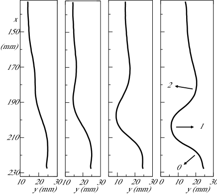
Figure 5: Variation of the fiber geometry during the fifth pinning event in Fig. 4a (lowest horizontal arrow). The leftmost (respectively rightmost) picture displays the shape of the fiber immediately after pinning (respectively before depinning). Time lapse between pictures: $0.166\ s$; total duration of trapping event: $1\ s$. Arrows: location of points of maximum curvature referred to as $0$, $1$ and $2$.

More information on the pinning-depinning process is obtained from the geometry of the fiber. The variations of the code color with time and distance in Fig. 3b indicate that, in contrast to the case of a smooth fracture (Fig. 3a), the fiber does not remain straight: it displays a buckling instability and meanders of shape and location varying with time appear. These variations are visualized directly in Figure 5 displaying the deformations of the fiber. During the pinning event, the tip of the fiber remains motionless while three bumps appear behind it; their amplitude increases with time while they propagate toward the tip. The deformation of the rear part of the fiber is much weaker while, in some cases, it gets translated sideways.

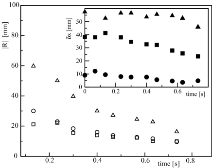
Figure 6: Variation with time of the absolute values $|R|$ of the radius of curvature of the fiber at the $3$ maximum curvature points designated by arrows in Fig. 5. Inset: time variation of the vertical distances $\delta x$ between these $3$ points and the fiber tip. Symbols for point $0$: ($\circ$,$\bullet$); for point $1$: ($\square$,$\blacksquare$) and for point $2$: ($\triangle$,$\blacktriangle$).

We characterized quantitatively the deformation of the fibers by the maximum absolute value $|R|$ of the radius of curvature in the three bumps and by the distance $\delta x$ of the corresponding points to the tip of the fiber (measured along axis $x$). The variation of $|R|$ and $\delta x$ with time for all three regions in this same experiment is displayed in Fig. 6. The distance $\delta x$ decreases with time with a relative velocity of the order of $10\,\mathrm{mm/s}$ lower than the fluid velocity ($160\,\mathrm{mm/s}$ in Fig. 4a) and similar for the three points of interest while the corresponding radii $|R|$ decrease strongly. The deformation is more important in the two first bumps for which the radius of curvature is of the order of $9.5\ \mathrm{mm}$ at the time when depinning occurs. These deformations reflect the accumulation of bending elastic energy behind the tip which, finally, gets large enough to overcome the friction forces with the wall. Similar scenarios were observed in all cases in which pinning takes place even though the time scales varies.

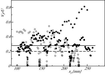
Figure 7: Variation of the ratio $V_{f}/U$ of the fiber and fluid velocity as a function of the distance $x_{t}$ from the inlet of model $F_{2}$ for three experiments with continuous fibers injected at a same location. ($\circ$) and ($\bullet$): water flowing at respective velocities $U=160\ \mathrm{mm/s}$ and $210\ \mathrm{mm/s}$. ($\ast$): flow of a polymer solution at $U=220\ mm/s$. Dotted and solid lines: average of fiber velocity over field of view respectively for $U=160$ and $210\ \mathrm{mm/s}$.

The pinning/depinning process should depend significantly on the hydrodynamic forces and, therefore, on the flow velocity $U$. This influence is analyzed in Figure 7 displaying the variation with distance of the normalized velocity $V_{f}/U$ of the fiber tip for two different values of $U$. At the lower velocity $U=160\,\mathrm{mm/s}$, the fiber displays a stop and go motion already visible qualitatively in Fig. 3 corresponding to the same experiment. The velocity cancels out at each pinning point and increases sharply after the release of the fiber to a value much higher than the time average (horizontal dashed line). For $U=210\,\mathrm{mm/s}$, the variations with time of the fiber velocity with respect to the mean value are of smaller amplitude (-100%,+50%) instead of (-100%,+150%). Also, the fiber only stops completely once while $V_{f}$ decreases by less than $40\%$ on other pinning sites: these are located at the same distances $x$ as for $U=160\,\mathrm{mm/s}$. These results imply that the influence on pinning of inertia forces dragging the fibers towards the walls is small. The normalized averages $\overline{V_{f}}/U$ of the fiber velocity with time are equal to $0.2$ and $0.28$ respectively for $U=160$ and $210\,\mathrm{mm/s}$. Even if the influence of the low velocity near the pinning sites is removed from this average, $\overline{V_{f}}/U$ is still only of the order of $0.3$ for both $U$ values. This is lower by a factor of $3$ than the values measured in model fractures with smooth plane walls (see Fig. 2).

IV Fiber transport by shear thinning fluids in rough model fractures

IV.1 Fiber transport in fracture $F2$

The influence of rheology has been studied specifically by replacing water by a shear thinning solution of characteristics discussed in section II.4 in the same model $F2$ as above. In Fig. 7, data obtained with this fluid are compared to the variations for water discussed in the previous section (the points of injection of the fibers are the same and correspond to the high aperture path). At a similar velocity ($\simeq 220\,\mathrm{mm/s}$), the ratio $V_{f}/U$ is larger for the shear thinning solution than for water, except at short distances. The amplitude of the velocity fluctuations is also smaller but they still take place at the same distances $x$ as the pinning sites observed in low velocity water experiments. The motion of the fiber remains therefore slightly influenced by the local asperities encountered along its path, although much less than for water.

Globally, using a shear thinning fluid instead of water reduces significantly the influence of the roughness of the walls on the motion of the fibers: their dynamics may be then much more similar to that reported in Sec. III.1 for the plane fracture $F1$. In particular, the increase of $V_{f}/U$ with the distance $x$ indicates that the reduced drag forces on the parts of the fiber located at the inlet influence the global motion of the fiber, like for fracture $F1$ but unlike the experiments of Sec. III.2 with water.

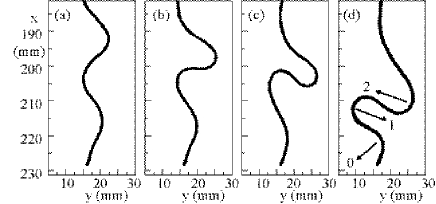
Figure 8: Variation of the fiber geometry during a pinning event for a polymer flow ($U=230\,\mathrm{mm/s}$) in the low aperture part of fracture $F2$. The leftmost (respectively rightmost) picture displays the shape of the fiber $0.1\ \mathrm{s}$ after pinning (respectively just before depinning). The definitions of points $0$, $1$ and $2$ are the same as in Fig. 5

The above results correspond to fibers moving, like in Sec. III.2, in the high aperture part of the width of the wedged fracture $F2$. However, fibers may propagate even in the low aperture part, if the fluid is shear thinning while they get blocked or build up side loops with water (see Fig. 4). The corresponding motion is then not continuous but of a “stop” and “go” type: the lower mean value of the aperture in these regions increases its relative fluctuations and there are more potential pinning sites. As already reported for water in Sec. III.2, a buckling instability occurs and fibers are deformed as they get pinned (Fig. 8). Like for water, these deformations are localized near the tip of the fiber and move towards it as they develop; their amplitude and curvature may however become significantly larger than for water before depinning takes place (see Fig. 5 for comparison). In Fig. 8, for instance, an overhang appears as bump $1$ is overtaken by $2$ as shown by the two upper sets of points in the inset. Also, the variation of the radius of curvature with time is more complex and not always monotonic (Fig. 9), reflecting the interaction between the different loops. The radii of curvature of loops $1$ and $2$ both become as low as $\simeq 2\,\mathrm{mm}$ or less: this is lower than the radius of loop $0$ and, also, much below the radii observed with water.

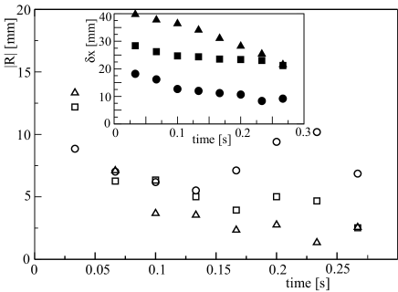
Figure 9: Variation with time of the radius of the fiber at the $3$ maximum curvature points designated by arrows in Fig. 8(d). Inset: time variation of the vertical distances $\delta x$ between these 3 points and the fiber tip. Symbols for point $0$: ($\circ$,$\bullet$); for point $1$: ($\square$,$\blacksquare$) and for point $2$: ($\triangle$,$\blacktriangle$).

These larger deformations may result both from the larger hydrodynamical forces in the polymer flow due to its higher mean viscosity and from the higher depinning energies in the narrow part of the wedge. The increased value of the hydrodynamical forces is also reflected in the faster variations of the distances $\delta x$ (see insets of Fig. 5 and Fig. 9).

IV.2 Fiber transport by shear thinning fluids in fracture with rough parallel walls.

IV.2.1 Aperture field and anisotropy of fracture $F3$.

The results of the previous section demonstrate that, using a polymer solution, it is possible to transport fibers along the full length of model $F2$, even in the lower mean aperture regions. The “wedge like” geometry of this model has allowed us to estimate the influence of the mean aperture $\bar{a}$ by varying the distance $y$ at the inlet of the model where the fiber is injected: however, this geometry may have unwanted effects like the sideways motions displayed in Fig. 4 and it may mask the influence of local aperture fluctuations. The present section deals therefore with experiments realized with another model ($F3$) using model rough walls with a similar geometry as $F2$ but with their mean planes parallel (see Figs. 10 for the corresponding aperture map and transverse mean aperture profile). As mentioned above, the fracture walls are two perfectly matching self-affine surfaces which are first put in contact and then pulled apart before introducing a small relative shear displacement.

As shown by several authors on Fracture Characterization and Flow (1996); Gentier et al. (1997); Yeo et al. (1998), this geometry results in an anisotropy of the aperture field and of the permeability: flow is easier in the direction normal to the shear displacement. In the present experiments, the mean flow ($x$ direction) is perpendicular to the shear ($y$ direction) and should therefore be oriented in the direction of highest permeability. The distribution of the color patches in the maps Fig. 10a-b indicates qualitatively that the distance over which deviations of the aperture from its mean value persist is larger along $x$ than along $y$. For instance, a long continuous vertical string of blue patches (corresponding to a high local aperture) is visible and is associated with a maximum in the transverse profile of Fig. 10c. This suggests a channelization effect related to the anisotropy of the permeability. Recent work has indeed shown Auradou et al. (2006, 2008) that, in this configuration, the flow field could be described approximately as a set of channels of constant hydraulic aperture and parallel to the direction $x$: this allowed, for instance, to predict the overall geometry of the displacement fronts between two miscible fluids. We shall analyze now how this feature influences the transport of fibers in model $F3$.

IV.2.2 Fiber transport in model $F3$.

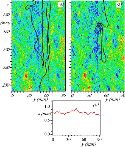
Figure 10: (a) Snapshots of $4$ fibers injected into a polymer flow in fracture $F3$ at different distances overlaid onto a map of the aperture field (mean fluid velocity $U=215\,\mathrm{mm/s}$). (b) Snapshot of a fiber coiled up after getting pinned inside the fracture ($U=242\,\mathrm{mm/s}$). A time sequence of the coiling process is displayed in Fig. 11. The color code corresponds to the aperture (red: $a\leq\,0.5\,\mathrm{mm}$, blue: $a\geq\,1.25\,\mathrm{mm}$). Field of view: $90\times 150\,\mathrm{mm}$. Distances in the vertical $x$ direction are counted from the top of the model (see Fig. 1). (c): variations of the aperture averaged along the distance $x$ parallel to the flow as a function of the transverse distance $y$.

In Figure 10a, snapshots of four fibers injected at different transverse distances $y$ are overlaid onto the aperture field of model $F3$. Three of them are weakly deformed and kept moving afterwards down to the lower end of the model. One notices that their location does not coincide exactly with the zone of highest aperture of the model although it is not far from it. The fourth fiber (at the left on the image) got pinned as it moved out of a high aperture region into a less open one; the shape of this fiber is also more strongly distorted, possibly reflecting a larger velocity gradient in the region where the fiber moves. In model $F3$, therefore, fiber transport is not solely determined by the distribution of the aperture even though it has a strong influence: other parameters like the local gradients of the aperture and slope of the surface or, yet, inertia effects may also be of importance. Some of the observations on fracture $F2$ previously suggested similar results.

IV.2.3 Irreversible pinning and fiber entanglement in model $F3$.

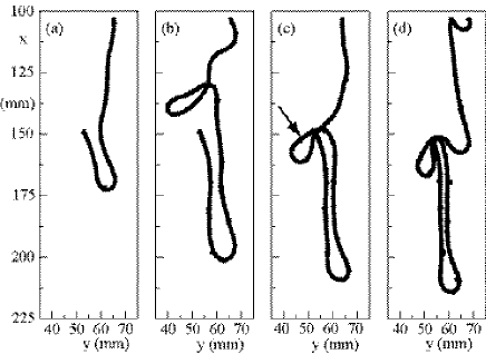
Figure 11: Evolution of the fiber as function of time during the build-up of a coil for the flow of a polymer solution in fracture $F3$ (see Fig. 10b). ¿From left to right, the time elapsed after pinning is respectively $0.63$, $1.13$, $1.3$ and $1.8\ s$.

Up to now, we have discussed mostly pinning events of finite duration like in Figs. 5 and 8. Irreversible pinning has however also been observed, for instance in the narrow parts of fracture $F3$; this often leads to an entanglement of the fiber around the pinning site and to the build up of intertwined loops like in Figs. 11 and 10b. Let us discuss in more detail the process leading to the configuration displayed in Fig. 10b following pinning in a narrower zone (yellow shade region near the top of the coil). At first, the fiber gets deformed like in the case of transient pinning (see Sections III.2 and IV.1 and Figs. 5 and 8). Then, while the tip remains pinned, bump $1$ overtakes it so that a loop appears at the right of the pinning site and move downwards (Fig. 11a). At the same time other parts of the fiber located farther upstream move leftwards and build up a second, closed loop (arrow in Fig. 11). A key point is the fact that the friction forces with the walls in the parts of the fiber located close to the pinning site are large enough to prevent hydrodynamic forces on fast moving parts of the fiber from dragging downward the rest of its length. Tension forces on the upstream parts are then quite low so that loops and deformations can easily appear. Finally, both loops move down: they get locked on the pinning site and dangle on both sides (Fig. 11c). This further reduces the tension on the upstream fiber sections so that new loops start to build up (Fig. 11d).

V Conclusion

In the present work, several clear-cut results have been obtained experimentally on the conditions for achieving the transport of flexible fibers in fractures. First, while in smooth fractures the friction of the fibers with the walls is negligible and does not influence their motion, its influence has been verified to be much stronger for rough walls: this may result in pinning and blockage or, at least, in a jerky progression instead of a continuous one.

Next, the aperture of the fracture (and particularly its ratio to the fiber diameter) is also a key factor, but with a more subtle influence than expected. On the one hand, in the wedge-shaped rough model $F2$ with a global transverse gradient of the mean aperture, fiber transport is, as expected, easier in the more open parts of the wedge than in narrower ones (however pinning may occur in open regions). In the rough fracture $F3$ with globally parallel walls and a channelized flow field, fiber motion is also easier in high permeability regions. On the other hand, the trajectory of the fibers does not coincide fully with the paths of highest aperture while pinning is also not always localized at minimal aperture points. Other factors such as the local slope of the walls and inertia forces pushing the fibers towards the solid surfaces must therefore play an important part. In the present experiments, the mobility of the fibers appears to increase with the mean flow velocity: further experiments will however be necessary to determine whether, at high velocities, some fibers may be forced into narrow zones by inertia effets and get blocked there.

In order to evaluate the transport of fibers in natural or industrial fracture systems of practical interest, different configurations of the aperture field need to be studied such as, for instance, a channelization perpendicular to the mean flow. Using our experimental set up, this may be investigated by changing the direction of the shear displacement between the two complementary rough walls with respect to the flow (more precisely by comparing for two identical complementary rough walls results obtained when the shear displacement $\vec{u}$ is parallel and perpendicular to the mean velocity $\vec{U}$). The value of Hurst’s exponent $H$ for the fracture walls may also influence fiber transport by determining the relative height of rugosities of different sizes in the plane of the fracture: it will be informative to compare the present measurements corresponding to $H=0.8$ to others achieved for $H=0.5$ (a value encountered in such materials as sandstone and sintered glass).

A third key observation is the enhancement of the mobility of the fibers when water is replaced by a shear thinning fluid at a same flow velocity. For instance, fiber propagation along the full length of rough fractures with a mean aperture of less than twice the fiber diameter becomes possible. Fiber motion is observed (although in a “stop and go” manner) in zones where they got stuck in water flows while, in regions of high aperture the displacement is faster and more continuous. Also, the influence of the interaction of the fibers with the walls is much reduced and the minimum value of the ratio of the mean aperture to the diameter of the fiber for observing transport is lower. This increased mobility in shear thinning flows may result from larger hydrodynamic forces (the effective viscosity of the polymer solutions is generally higher than that of water). Other possible explanations must however be investigated : for instance, the fiber is more frequently localized in the center of the gap between the walls than in Newtonian fluids. Also, at high velocities, a layer of low viscosity Newtonian fluid appears near the walls and may influence the transport of the fibers. In order to understand this effect, it will be also important to compare the present results with those obtained with Newtonian fluids of different viscosities and other non Newtonian fluids such as shear-thinning fluids with different characteristic exponents and yield stress or viscoelastic fluids.

The transport of fibers is also strongly influenced by their deformation under the effect of hydrodynamic forces which is particularly important during pinning events. In the case of intermittent pinning marked by a jerky motion, the amplitude of the deformation of the fiber increases with time and the elastic energy accumulates until the front tip is released and the fiber recovers roughly its initial shape. The amplitude of the deformations and the curvatures observed were larger for experiments with the polymer solution than for water. In the case of permanent pinning, the amplitude of the deformations may increase further: loops appear and pile up on the pinning site, finally leading to entanglement. These results show qualitatively that, even for very flexible fibers, the influence of the elastic modulus on their transport by the flow cannot be neglected.

In future work, systematic investigations will be needed to characterize more quantitatively the dependence of the pinning and entanglement processes on the control parameters of the experiments. A first important question is the dependence of the motion of the fibers on their flexibility and on the value of their diameters compared both to the mean fracture aperture $\overline{a}$ and to its standard deviation $\sigma_{a}$. Pinning effects also depend clearly on the interaction of the fibers and the walls: this involves friction between them as well as well as blockage of the fiber motion by the wall roughness: their relative magnitude will need to be investigated. Overall, as shown for instance by Fig. 7

Finally, while the present experiments greatly help to determine the conditions and characteristics for fiber transport in single fractures, further work will be needed to understand their transfer from one fracture to another in a fracture network.