Scaling behavior of the disordered contact process

Abstract

The one-dimensional contact process with weak to intermediate quenched disorder in its transmission rates is investigated via quasi-stationary Monte Carlo simulation. We address the contested questions of both the nature of dynamical scaling, conventional or activated, as well as of universality of critical exponents by employing a scaling analysis of the distribution of lifetimes and the quasi-stationary density of infection. We find activated scaling to be the appropriate description for all disorder strengths considered. Critical exponents are disorder dependent and approach the values expected for the limit of strong disorder as predicted by strong-disorder renormalization group analysis of the process. However, even for the strongest disorder under consideration no strong-disorder exponents are found.

The critical behavior of systems with quenched randomness has been the subject of interest for a long time. Over the past decades, their investigation has revealed rich behavior including the existence of new phases Griffiths (1969), novel fixed points Igloi and Monthus (2005), and unconventional scaling properties Fisher (1987).

Recently, attention has turned towards the influence of disorder on stochastic many-particle systems with a phase transition into an absorbing state owing to their relevance in physics, chemistry and biology Hinrichsen (2000a). In particular, the contact process (CP) Harris (1974), a paradigmatic model for the stochastic spreading of an infectious disease, has been investigated as a representative for the prominent universality class of directed percolation (DP). Interest in the influence of disorder on this process was sparked by the surprising lack of experimental observation of DP behavior in real systems, for which disorder may be responsible Hinrichsen (2000b). With a recent study presenting convincing evidence of DP critical behavior in turbulent liquid crystals Takeuchi et al. (2007), an understanding of the effects of disorder is more relevant than ever.

Initial Monte Carlo (MC) studies of the disordered CP (DCP) found continuously varying dynamical critical exponents assuming conventional scaling Noest (1986); Moreira and Dickman (1996); Cafiero et al. (1998). Recently, deep insight was gained through a strong-disorder renormalization group study of the DCP which revealed an infinite-randomness fixed point (IRFP) for sufficiently strong disorder in close analogy to the random transverse-field Ising model Hooyberghs et al. (2003). While this makes the strong-disorder limit of the process well understood Igloi and Monthus (2005) and predicts new strong-disorder exponents as well as an unconventional “activated” form of dynamical scaling, the behavior in the weak- and intermediate-disorder regime remains a subject of debate Hooyberghs et al. (2004); Vojta and Dickison (2005). Initial density-matrix renormalization group (DMRG) studies were not able to convincingly distinguish the two alternative dynamical scaling scenarios, conventional or activated, and reported critical exponents continuously changing with disorder strength Hooyberghs et al. (2004). In contrast, a recent MC study reported evidence for activated scaling with strong-disorder exponents for all disorder strengths Vojta and Dickison (2005).

Static scaling in the DCP was found to be of conventional form Dickman and Moreira (1998) as predicted by the strong-disorder renormalization study Hooyberghs et al. (2003). However, there exists conflicting evidence as to the universality of the exponents for weak and intermediate disorder with the literature reporting both disorder-dependent Dickman and Moreira (1998); Neugebauer et al. (2006) and strong-disorder Vojta and Dickison (2005) exponents.

In this paper, we aim to address both the question of the type of dynamical scaling as well as of universality of exponents in the weak- and intermediate-disorder regime by considering the scaling of the distribution of lifetimes, $P(\tau)$, of the 1d DCP obtained from quasi-stationary MC simulation. This is motivated by the fact that an analysis of the scaling behavior of entire distributions promises to yield clearer results as compared to the scaling of means Young and Rieger (1996); Hooyberghs et al. (2004). Further, in dynamic single-seed MC simulations employed for the DCP in the past Moreira and Dickman (1996); Vojta and Dickison (2005), the question of whether the long-time limit of the process had been reached was frequently contested. In contrast, quasi-stationary simulations offer a clear means of ensuring this: a true stationary average whose convergence can be monitored.

In the clean CP (without disorder) defined on a lattice, sites represent the individuals of a population which can be in two possible states, susceptible or infected. An infected site attempts to spread its infection to nearest neighbors at rate $\lambda$, while recovery is spontaneous at rate $\epsilon=1$. In the limit $t\to\infty$ for an infinite system, there exist two distinct states: an active one where a finite density $\rho$ of infected sites remains and a non-active regime in which the system ultimately gets trapped in an absorbing state with no infected sites remaining. The system undergoes a continuous phase transition between these two phases at a critical rate $\lambda-\lambda_{c}^{0}\equiv\Delta=0$ with order parameter $\rho$ Hinrichsen (2000a); Marro and Dickman (1999).

Starting from a fully-infected system, the density of infected sites initially relaxes while spatial correlations grow towards the size of the system and temporal correlations decay. Once the correlation length becomes comparable to this size, the process enters a quasi-stationary (QS) regime. This metastable state is characterized by a non-zero time-independent transition rate to the absorbing state. Given that no true non-trivial stationary state can exist in a finite system, in these cases QS averages are commonly used as a proxy in the CP and allied models. Ultimately, the clean CP is bound to enter the absorbing state, the approach of which is characterized by an exponentially decaying probability of survival, $P_{s}(t)\sim\exp(-t/\tau)$, with a characteristic lifetime $\tau$. In the active state, $\Delta>0$, this lifetime is known to obey finite-size scaling,

$$\tau\sim N^{z}\exp\left(N^{d}\Delta^{\nu_{\perp}d}\right)~{},$$ (1)

where $z$ and $\nu_{\perp}$ are critical exponents while $N$ denotes the size of the system. Further, the QS density of infected sites, $\overline{\rho}$, obeys a similar scaling form characterized by the universal scaling function $F$, i.e.

$$\overline{\rho}\sim N^{-x}F\left(\Delta N^{-1/\nu_{\perp}}\right)~{},$$ (2)

with $x=\beta/\nu_{\perp}$, where $\beta$ is the order parameter exponent in the infinite system defined via the behavior of the control parameter in the vicinity of the critical point, $\rho\sim\Delta^{\beta}$ Marro and Dickman (1999); Dickman and Moreira (1998).

Turning to the disordered process, we follow Ref. Vojta and Dickison (2005) and incorporate quenched randomness into the transmission rates of individual sites $i$, $\lambda_{i}$, which are drawn from the bimodal distribution

$$P(\lambda_{i})=(1-p)\delta(\lambda_{i}-\lambda)+p\delta(\lambda_{i}-c\lambda)~{},$$ (3)

where $p$ controls the concentration of impurities while $0<c<1$ characterizes the strength of the disorder. As $c<1$, a particular realization of the disorder contains a concentration $p$ of randomly arranged impurity sites which are less active than the surrounding sea of host sites. As a consequence, there now exists a new dirty critical point at a rate $\lambda_{c}>\lambda_{c}^{0}$. Also, observables may in general take different values between different realizations leading to disorder-induced distributions such as $P(\tau)$ for the lifetime.

Scaling predictions for $P(\tau)$ exist and differ for the two alternative scaling scenarios, i.e. conventional and activated scaling. In the former case, the relevant variable is $\tau$ and its average over disorder, $\langle\tau\rangle$, is expected to obey a scaling form analogous to Eq. (1) albeit with a possibly disorder-dependent dynamical exponent $z$. Accordingly, the appropriate scale-invariant combination of variables is $\tau N^{-z}$ and the lifetime distribution at criticality is expected to scale as

$$P(\tau)=N^{-z}\tilde{P}(\tau N^{-z})~{},$$ (4)

where $\tilde{P}$ is a universal scaling function.

Systems that exhibit activated scaling are characterized by a strong dynamical anisotropy: the typical length-scale is related to the logarithm of the typical timescale, thus rendering the dynamical exponent formally infinity. This reflects the notion that the very broad distributions for observables are better described by their geometric rather than arithmetic means Igloi and Monthus (2005). For the lifetime, this leads to a scaling combination $N^{-\Psi}\ln(\tau)$ and a corresponding scaling relation Hooyberghs et al. (2003),

$$P(\ln(\tau))\sim N^{-\Psi}\tilde{P}(N^{-\Psi}\ln(\tau))~{},$$ (5)

where $\Psi$ is an activated scaling exponent [cf. Eq. (4)]. For an IRFP, which is known to control the critical behavior of the DCP for sufficiently strong disorder, the exponent takes the value $\Psi=\frac{1}{2}$. This type of fixed point is characterized by an extreme dynamical anisotropy, ultra-slow dynamics and distributions whose width diverges with system size Igloi and Monthus (2005); Vojta (2006).

The QS density $\overline{\rho}$ is expected to follow a conventional scaling form analogous to Eq. (2) with an exponent $x$ which differs from the clean DP value and, for sufficiently strong disorder, is predicted to be $x=\frac{3-\sqrt{5}}{4}\approx 0.19$ Hooyberghs et al. (2003).

In order to check the above scaling relations for the DCP, the QS state can be investigated numerically. Analysis of this metastable state in computer simulations has proved to be notoriously difficult in the past. Commonly, the time-dependent density of infected sites conditioned on survival, which becomes stationary in the QS regime, is investigated Marro and Dickman (1999). Problematically though, it is neither clear a priori at what time an observable like the average density of infected sites $\overline{\rho}$ has converged to its QS value nor when the QS state starts to decay due to finite size effects Lübeck and Heger (2003). Therefore, a range of alternative approaches have been proposed which enable an observation of this metastable regime (see Ref. de Oliveira and Dickman (2005a) and references therein). Here, we employ the QS simulation method de Oliveira and Dickman (2005a) which allows a direct sampling of the QS state by eliminating the absorbing state and redistributing its probability mass over the active states according to the history of the process. The modified process possesses a true stationary state which corresponds to the original QS state and allows a precise measurement of QS observables. Generally, the method has proved to be efficient with fast and reliable convergence after optimization of history sampling parameters. As demonstrated in Ref. de Oliveira and Dickman (2005b), the lifetime of the QS state can be determined as the inverse of the rate of attempts by the system to enter the absorbing state.

In order to investigate the validity of the two different scaling scenarios for the lifetime distribution at the dirty critical point, simulation data for disorder strengths $c=0.2,0.4,0.6$ and $0.8$ at a concentration $p=0.3$ were considered at the critical rates reported in Ref. Vojta and Dickison (2005). System sizes of $N=16,32,64$ and $128$ sites were investigated with data sampled from no less than $10^{4}$ disorder realizations per system size and QS simulation times of up to $10^{9}$ time steps. Given that probability density functions (PDFs) are difficult to obtain from simulation data (as binning procedures have to be used which may introduce artifacts), we perform scaling on cumulative density functions (CDFs), $F_{\tau}(t)=\int_{0}^{t}P(t^{\prime})\,\text{d}t^{\prime}$. The scaling properties of these can be derived by starting from the two scaling forms for conventional and activated scaling, given by Eqs. (4) and (5), respectively, where for the former case

$$F_{\tau}(t)=\int_{0}^{t}N^{-z}~{}\tilde{P}(t^{\prime}N^{-z})\,\text{d}t^{\prime}=\tilde{Q}(tN^{-z})~{},$$ (6)

with $\tilde{Q}(x)$ a new scaling function. An analogous expression follows for the case of activated scaling with $\tau$ replaced by $\ln(\tau)$.

As displayed in Fig. LABEL:fig:tau_dirty, the resulting CDFs were collapsed onto each other according to the two possible scaling scenarios (main panels). In order to achieve a fair comparison, logarithmic variables were used for the conventional scaling case Young and Rieger (1996). As illustrated in Fig. 2, the exponents $\Psi$ and $z$ were determined from a power-law fit to the appropriate scaling forms for the mean in the two scenarios, i.e. $\langle\ln(\tau)\rangle\sim N^{\Psi}$ and $\langle\tau\rangle\sim N^{z}$. Insets show the alternative collapse using PDFs as discussed above which requires the use of histograms. There, the size of bins was chosen in order to minimize noise and the smooth curve was obtained by Gaussian broadening of individual data points.

For the case of strongest disorder ($c=0.2$, $\lambda_{c}=5.24$), least-squares fitting gave exponents $\Psi_{c=0.2}=0.29(2)$ and $z_{c=0.2}=3.44(3)$ for the two scaling scenarios, respectively. Data collapses for the distributions are shown in Fig. LABEL:fig:tau_dirty_c0.2 for both activated (top panel) and conventional scaling (bottom panel). From these results, we judge that the activated scaling scenario provides a better fit to the data. In particular, while the collapse is not perfect, it is not found to exhibit any systematic trends which would hint at a fundamental inconsistency with the scaling form. This is also confirmed by the inset which shows the corresponding collapse of the PDF. Generally, while the fit is excellent for small to medium values of $\tau$, it gets worse with increasing $\tau$. We attribute this to the fact that large values of $\tau$ correspond to rare events causing the tail of the distribution to have been sampled at a comparatively poorer density than the bulk which results in stronger fluctuations. Considering the collapse using the conventional scaling form [bottom panel of Fig. LABEL:fig:tau_dirty_c0.2] on the other hand produces a clear trend of shifting of distributions between different system sizes indicating a worse collapse as compared to the previous case for both CDF and PDF.

Looking at an analogous analysis for the case of weakest disorder ($c=0.8$, $\lambda_{c}=3.525$) in Fig. LABEL:fig:tau_dirty_c0.8, the two scaling scenarios become harder to differentiate. A collapse using the measured exponents $\Psi_{c=0.8}=0.22(2)$ and $z_{c=0.8}=1.65(3)$ appears to work similarly well in both cases but the quality of collapse is too poor to allow any definitive judgment. A close look reveals a systematic trend of shifting curves for the case of conventional scaling [bottom panel in Fig. LABEL:fig:tau_dirty_c0.8] while crossings appear to be less systematic in the activated scaling picture [top panel in Fig. LABEL:fig:tau_dirty_c0.8]. Therefore, slight preference may be given to the activated scaling scenario.

In addition, the intermediate cases of both $c=0.4$ and $c=0.6$ (not shown) were considered in an analogous fashion and showed an excellent activated scaling collapse of similar quality as for the case of $c=0.2$. Collapsing data for all disorder strengths considered on the same plot shows no universality of the scaling function between different disorder strengths, i.e. it appears to be disorder dependent.

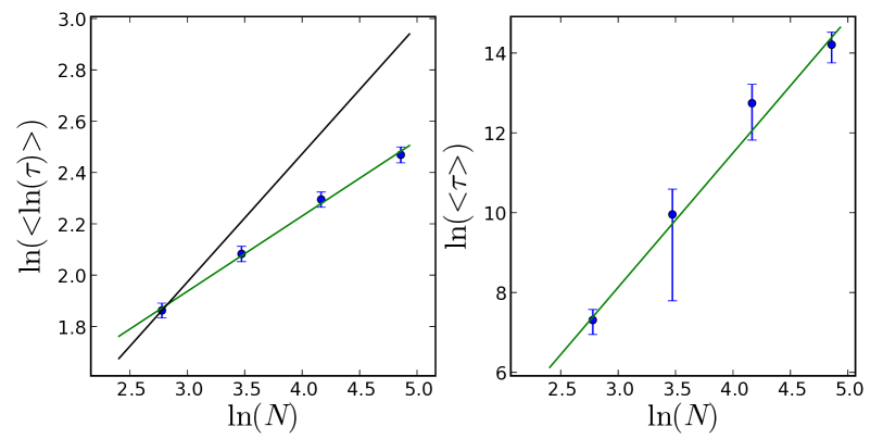
Figure 2: (Color online) Example of the scaling of the average $\langle\ln(\tau)\rangle$ (left) and $\langle\tau\rangle$ (right) with system size for the case of strongest disorder ($c=0.2$) used to extract the exponents $\Psi$ and $z$.

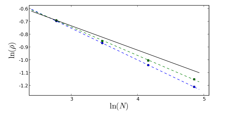
Figure 3: (Color online) The quasi-stationary density $\overline{\rho}$ as a function of system size $N$ at criticality for both the strongest (top, $c=0.2$) and the weakest (bottom: $c=0.8$) disorder strength. Dashed lines are linear least-squares fits which gave slopes of $x_{c=0.2}=0.22(1)$ and $x_{c=0.8}=0.25(1)$ while the solid line is a guide to the eye with slope $x_{\text{strong}}=0.19$, the expected exponent in the strong-disorder limit.

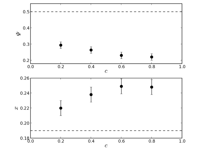
Figure 4: (Color online) Critical exponents $\Psi$ (top panel) and $x$ (bottom panel) as a function of disorder strength $c$ where dashed lines show the values in the limit of strong disorder.

Finite-size scaling of the QS density $\overline{\rho}(N)$, as shown in Fig. 3, is found to be conventional with a disorder-dependent exponent $x=x(c)$. The conventional scaling form is in line with previous investigations Dickman and Moreira (1998) and theoretical predictions Hooyberghs et al. (2003). Moreover, the fact that we again find continuously varying exponents gives additional credibility to the scaling picture presented above. Generally, both the exponent $\Psi$ and the exponent $x$ are found to approach their values predicted from strong-disorder renormalization Hooyberghs et al. (2003) with increasing strength of disorder starting from their homogeneous values as shown in Fig. 4. For the strongest disorder under consideration ($c=0.2$), both exponents are found to still be well away from their predicted strong-disorder values.

The above findings suggest that for strong enough disorder, activated scaling captures the behavior of the disordered CP well compared to a conventional scaling picture. For weak disorder however, no such clear conclusion can be made. Further, associated critical exponents appear to change smoothly from their clean DP values approaching their values characteristic of an IRFP asymptotically with increasing disorder strength. While this conclusion appears to be in conflict to that presented in Ref. Vojta and Dickison (2005), the authors of that reference do discuss doubts about the universality of exponents and cannot exclude the possibility of a change with disorder strength. We have re-analyzed some of the data presented there and found it to be compatible with our exponent values.

There exist three possible explanations compatible with these findings. First, a continuous line of fixed points, one for each strength of disorder, could be present which for sufficiently strong disorder turns to an attractive flow into the IRFP as suggested in Ref. Hooyberghs et al. (2003). Second, identical and numerically indistinguishable behavior could be explained by a crossover between the clean DP fixed point and the IRFP where effective exponents are observed at intermediate disorder strengths due to the influence of both fixed points. This has been observed in several disordered equilibrium systems as discussed in e.g. Refs. Carlon et al. (2001); Fisher (1974). Lastly, in principle, the observed behavior could also be explained by an abrupt jump from the clean DP exponents to those of the IRFP obscured by finite-size corrections.

The last option we feel can be excluded in light of the facts that perturbative series expansions (cf. Ref. Neugebauer et al. (2006)) do not show a jump in exponents and that no evidence for strong corrections to finite-size scaling were observed by us. At the same time, the other two scenarios are compatible with our and most other results but cannot be safely distinguished by numerical investigation alone without an established theoretical framework for the crossover in the DCP.

We would like to thank Ronald Dickman for helpful remarks. Also, we thank Allon Klein, Chris Neugebauer and Francisco Pérez-Reche for stimulating discussions. The computations were performed on the Cambridge High Performance Computing Facility. SVF would like to thank the UK EPSRC and the Cambridge European Trust for financial support.

References

- Griffiths (1969) R. B. Griffiths, Phys. Rev. Lett. 23, 17 (1969).
- Igloi and Monthus (2005) F. Igloi and C. Monthus, Phys. Rep. 412, 277 (2005).
- Fisher (1987) D. S. Fisher, J. Appl. Phys. 61, 3672 (1987).
- Hinrichsen (2000a) H. Hinrichsen, Adv. Phys. 49, 815 (2000a).
- Harris (1974) T. E. Harris, Ann. Prob. 2, 969 (1974).
- Hinrichsen (2000b) H. Hinrichsen, Braz. J. Phys. 30, 69 (2000b).
- Takeuchi et al. (2007) K. A. Takeuchi, M. Kuroda, H. Chaté, and M. Sano, Phys. Rev. Lett. 99, 234503 (2007).
- Noest (1986) A. J. Noest, Phys. Rev. Lett. 57, 90 (1986).
- Moreira and Dickman (1996) A. G. Moreira and R. Dickman, Phys. Rev. E 54, R3090 (1996).
- Cafiero et al. (1998) R. Cafiero, A. Gabrielli, and M. A. Muñoz, Phys. Rev. E 57, 5060 (1998).
- Hooyberghs et al. (2003) J. Hooyberghs, F. Iglói, and C. Vanderzande, Phys. Rev. Lett. 90, 100601 (2003).
- Hooyberghs et al. (2004) J. Hooyberghs, F. Iglói, and C. Vanderzande, Phys. Rev. E 69, 66140 (2004).
- Vojta and Dickison (2005) T. Vojta and M. Dickison, Phys. Rev. E 72, 036126 (2005).
- Dickman and Moreira (1998) R. Dickman and A. G. Moreira, Phys. Rev. E 57, 1263 (1998).
- Neugebauer et al. (2006) C. J. Neugebauer, S. V. Fallert, and S. N. Taraskin, Phys. Rev. E 74, 040101(R) (2006).
- Young and Rieger (1996) A. P. Young and H. Rieger, Phys. Rev. B 53, 8486 (1996).
- Marro and Dickman (1999) J. Marro and R. Dickman, Nonequilibrium Phase Transitions in Lattice Models (Cambridge University Press, Cambridge, 1999).
- Vojta (2006) T. Vojta, J. Phys. A 39, R143 (2006).
- Lübeck and Heger (2003) S. Lübeck and P. C. Heger, Phys. Rev. E 68, 056102 (2003).
- de Oliveira and Dickman (2005a) M. M. de Oliveira and R. Dickman, Phys. Rev. E 71, 016129 (2005a).
- de Oliveira and Dickman (2005b) M. M. de Oliveira and R. Dickman, Braz. J. Phys. 36, 3A (2005b).
- Carlon et al. (2001) E. Carlon, P. Lajko, and F. Igloi, Phys. Rev. Lett. 87, 277201 (2001).
- Fisher (1974) M. E. Fisher, Rev. Mod. Phys. 46, 597 (1974).