Central Forests in Trees

Abstract

A new $2$-parameter family of central structures in trees, called central forests, is introduced. Minieka’s $m$-center problem [10] and McMorris’s and Reid’s central-$k$-tree [8] can be seen as special cases of central forests in trees. A central forest is defined as a forest $F$ of $m$ subtrees of a tree $T$, where each subtree has $k$ nodes, which minimizes the maximum distance between nodes not in $F$ and those in $F$. An $O(n(m+k))$ algorithm to construct such a central forest in trees is presented, where $n$ is the number of nodes in the tree. The algorithm either returns with a central forest, or with the largest $k$ for which a central forest of $m$ subtrees is possible. Some of the elementary properties of central forests are also studied.

Keywords:

central forest, center, tree, $m$-center, central-$k$-tree, algorithm, location problems, network center problems

1 Introduction

Graph theory has applications in many real life situations. One of the very interesting applications of graph theory is the theory of facility location in networks. Graph theorists often focus on (unweighted) graphs, particularly trees. In the real world, there are a lot of networks that are organized into trees, such as ethernet-based campus/enterprise networks, core networks of cellular networks and telephone networks. These applications are based on the centrality in trees. There are many kinds of centrality notions like center of tree, defined by Jordan [6] as a set of nodes that minimizes the maximum distance to other nodes, centroid of a tree, again defined by Jordan [6] as the set $x$ of nodes of tree $T$ that minimizes the maximum order of a component of $T-x$ and median of tree, defined by Zelinka [23] as the set of nodes that minimizes the sum of distances or equivalently the average distance to other nodes.

Minieka [10] considered an $m$ center of a tree $T$ as a set $M$ of $m$ nodes of the tree that minimizes the maximum distance between every other node of $T$ and $M$. Chandrasekaran and Tamir [3] presented an algorithm for locating $m$ facilities on a tree network to minimize the maximum distance of the nodes on the network and their nearest node in $m$-center. This algorithm takes $O((n\log m)^{2})$ time with $n$ nodes in the network. Nimrod and Tamir [9] presented an improvement on the previous algorithms for locating $m$ facilities. An $O(n\log^{3}n)$ algorithm was presented for continuous $m$-center problem in trees. They also presented an $O(n\log^{2}n\log\log n)$ algorithm for a weighted discrete $m$-center problem. Steven et. al. [1] gave a self-stabilizing algorithm for locating centers and medians of trees. Kariv and Hakimi [7] presented an $O(n\cdot\lg n)$ algorithm for finding the (node or absolute) 1-center; an $O(n)$ algorithm for finding a (node or absolute) dominating set of radius $r$ and an $O(n^{2}\cdot\lg n)$ algorithm for finding a (node or absolute) $m$-center for any $1<m<n$ for node-weighted tree. Kariv and Hakimi [7] also proposed an $O(n\cdot\lg^{m-2}n)$ algorithm for finding an absolute $m$-center (where $3\leqq m<n$) and an $O(n\cdot\lg^{m-1}n)$ algorithm for finding a node $m$-center (where $2\leqq m<n$) for a node unweighted tree.

Tamir [21] studied the use of dynamic data structures on obnoxious center location problems on trees, and on the classical $m$-center problem on general networks, deriving better complexity bounds in both the cases. Again in 1991, Tamir [22] showed that the continuous $m$-Maximin and $m$-Maxisum dispersion models are NP-hard for general (nonhomogeneous) graphs. Burkard et. al. [2] offered an improvement over Tamir’s work by giving a linear-time algorithm for graph that is a path or a star. Their algorithm is an improvement over Tamir’s [21] by a factor of log($n$) for general trees.

Slater [18, 16, 19] considered the location facility problem that was path shaped on a tree. Locating paths with minimum eccentricity and distance, respectively, may be viewed as multicenter and multimedian problems, respectively, where the facilities are located on nodes that must constitute a path. A linear algorithm for finding paths with minimum eccentricity is also presented. Hedetniemi et. al.  [5] gave a linear time algorithm for finding the minimal path among all paths with minimum eccentricity in a tree network. Morgan and Slater [13] considered the problem of finding a path of minimum total distance to all other nodes in a tree network with equal as well as non-equal arc lengths. Minieka [11] considered central paths and trees with fixed length $L$ in a tree network. Slater [15, 17] studied centers to centroids and $k$-nucleus of a graph and also Reid [14] considered centroids to centers in trees.

Along with these central sets, $k$-center and $k$-median as given in Handler and Mirchandani [4] and Mirchandani and Francis [12] are of interest in facility location theory. McMorris and Reid [8] considered a central $k$-tree is a subtree $C$ of $k$ nodes that minimizes the maximum distances between nodes not in $C$, and those in $C$.

In this paper, we generalize the work done by Minieka [10] and McMorris and Reid [8], by considering a forest $F$ of $m$ subtrees of a tree $T$, where each subtree has $k$ nodes, where $F$ minimizes the maximum distance between nodes not in $F$ and those in $F$. We introduce this generalization as central forests in trees. Minieka’s [10] and McMorris’s and Reid’s [8] work can be seen as special cases of central forest in trees. An $O(n(m+k))$ algorithm to construct such a central forest in trees is presented, where $n$ is the number of nodes in the tree. The complete performance analysis and proof of correctness are given. We study some of the elementary properties of central forest. We also have the upper bound on the order of subtrees in central forests as our algorithm either returns with a central forest, or with the largest $k$ for which a central forest of $m$ subtrees is possible.

Section 2 talks about the notations and the work done by Minieka [10] and McMorris and Reid [8] in detail. Section 3 defines formally the central forests in trees. Some of the properties of central forest and the upper bound on the order of subtrees in central forests are also discussed in this section. Section 4 presents algorithm to construct central forest in trees along with performance analysis and proof of correctness. This section also includes an example demonstrating the working of algorithm. Section 5 concludes the paper and also provides some pointers for future work.

2 Preliminaries

2.1 Notation

Definition 2.1.

The definitions of some of the terms used throughout the paper are as follows:

• A graph $G$ is an ordered pair $(V(G),E(G))$, where $V(G)$ is a finite nonempty set of nodes, and $E(G)\subseteq\{\{v,v^{\prime}\}\ |\ v,v^{\prime}\in V(G),v^{\prime}\neq v\}$ is the set of edges.

• The number of nodes in $G$ is called the order or size of $G$.

• Let $e=\{v,v^{\prime}\}$ be an edge; we say that $e$ is incident with $v$ and $v^{\prime}$, that $v^{\prime}$ is a neighbor of $v$, or that $v^{\prime}$ is adjacent to $v$. Two edges are adjacent if they share a common node.

• The degree of a node $v$, denoted $degree(v)$, is the number of edges incident with $v$. All nodes of degree 1 are called leaves or end-nodes, while other nodes are internal nodes.

• A path $P$ from $v_{1}$ to $v_{i}$ in $G$ is an alternating sequence $P\ \triangleq\ v_{1},e_{1},v_{2},e_{2},$ $\ldots,e_{i-1},v_{i}$ of nodes and edges such that $v_{1},v_{2},\ldots,v_{i}$ are distinct, and for every $j$, $1\leq j<i$, $e_{j}$ is an edge incident with nodes $v_{j}$ and $v_{j+1}$; $i-1$ is the length of $P$. If there exists such a path in $G$ such that $\{v_{i},v_{1}\}$ is also an edge of $G$, then $P$ together with this edge is a cycle of length $i$.

• A graph is connected if there is a path between any two nodes.

• The distance between nodes $v_{i}$ and $v_{j}$, denoted $d(v_{i},v_{j})$, is the length of a shortest path between them.

• The degree of a graph $G$, denoted $\Delta(G)$, is the maximum degree of any node in $G$.

• If $G$ and $G^{\prime}$ are graphs, $G^{\prime}$ is a subgraph of $G$ if $V(G^{\prime})\subseteq V(G)$ and $E(G^{\prime})\subseteq E(G)$.

• A connected component of a graph $G$ is a maximal connected subgraph of $G$.

• A graph that is connected and has no cycles is called a tree.

• The eccentricity of a node $x$ in a connected graph $G$, denoted $e(x)$, is given by:

  $$e(x)\ \triangleq\ \mathrm{max}\{d(x,y)\ |\ y\in V(G)\}.$$

• If $V\subset V(T)$, the subtree induced by $V$ can be defined in two ways:

  • The subgraph of $T$ induced by $V$ is the forest with node set $V$ and edge set given by all edges of $T$ with both ends in $V$.

  • The subgraph of $T$ induced by $V$ is the smallest subtree of $T$ containing all nodes of $V$.

• A forest in a graph is a disjoint union of trees. In trees, a forest is a disjoint union of subtrees.

2.2 Center

Center of a graph $G$, denoted by center($G$) is defined as follows:

Definition 2.2.

If $c\subseteq V(G)$ and $|c|=1$ or $2$, then

$$center(G)\ \triangleq\ \{c\ |\ c\in V(G),e(c)\leq e(y),\ \forall y\in V(G)\}.$$

In other words, the center of a graph is a set of nodes that minimizes the maximum distance to other nodes of the graph. For trees, Jordan [6] has given a pruning algorithm to find the center. The algorithm works in steps. In each step, the end (leaf) nodes of the tree and their connecting edges are removed to get a new tree. When we keep on pruning the tree like this, we are left with either a single node or two nodes joined by an edge. This set of $1$ or $2$ nodes is the unique center of the tree. This set of nodes has the minimum eccentricity. In the Figure 1, the dashed edges show the nodes pruned at the first step and the dotted edges denote the nodes pruned at the second step of the algorithm. At the third step only a single node is left, and that is the unique center of the tree. For clarity, the central node of tree is indicated by an oval around it.

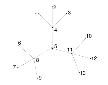
Figure 1: An example of a center of a tree

2.3 $m$-Center

Minieka [10] has generalized the concept of a central node of a tree $T$ as follows:

Definition 2.3.

If $X\subseteq V(T)$ and $u\in V(T)$, define

$$d(u,X)\ \triangleq\ \mathrm{min}\ d(u,x_{i}),\ x_{i}\in X$$

$$e(X)\ \triangleq\ \mathrm{max}\ d(u,X),\ u\in V(T)$$

$$center_{m}(T)\ \triangleq\ \{X\ |\ e(X)\leq e(Y),\ \forall\,Y\subseteq V(T),|Y|=m\}$$

Minieka [10] defines the $m$-center by “an $m$-center set of a graph is any set of $m$ nodes, belonging to either the nodes or edges, that minimizes the maximum distance from a node to its nearest node in $m$-center.” In other words, the problem of $m$-center for $m$ = $1,2$…, is to find the set of nodes $X$ that minimizes the maximum distance between a node of $G$ and its nearest node in $m$-center.

The members of set $X$ are called as $m$-center of tree $T$. The set $X$ need not be unique. Minieka has also given a method for solving the $m$-center problem by solving a finite series of minimum set covering problems. An example of an $m$-center is as shown in Figure 2 for $m=3$. In this figure nodes $4,8$ and $11$ makes up the $3$-center of the tree, i.e. here $X$ = {$4,8,11$}.

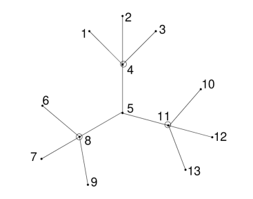
Figure 2: An example of a $3$-center of a tree

NB: In the literature, an $m$-center of the tree (graph) is also sometimes known as the $p$-center of the tree (graph). But, as Minieka originally proposed it as $m$-center, we are using the term $m$-center instead of $p$-center.

Remark 2.4.

We need to impose the further restriction that $\Delta T\leq m$.

The justification for this is that if the restriction is not observed, then for some trees, e.g., a star of degree $\Delta(T)$, the $m$-center may not be properly defined. $\Delta T$ nodes in a star can be properly placed as nodes of the $m$-center, but if $m>\Delta T$, then by the pigeonhole principle, at least one limb of the star must have more than one node belonging to the $m$-center, which is not sensible.

2.4 Central $k$-Trees

Central $k$-trees were introduced by McMorris and Reid in 1997 [8].

Definition 2.5.

If the tree $T$ be of order $n$ and $W_{T,k}$ be the set of all the subtrees of $T$ of order $k$, then a central-$k$-tree is defined as

$$\mathrm{Central}--k--\mathrm{tree}(T)\ \triangleq\ \{W\ |\ e(W)\leq e(W^{\prime}),\ \forall W^{\prime}\in W_{T,k},k\leq n\}.$$

Figure 3: An example of a central-$4$-tree of a tree

An example of central-$k$-tree is shown in Figure 3 for $k=4$. The algorithm for central-$k$-tree for tree $T$, from their paper is given as algorithm Central-$k$-tree. The tree $T$ of Figure 2, when pruned as per algorithm Central-$k$-tree, yields a central-$4$-tree as depicted in Figure 3. The pruned edges are shown as dotted lines.

The pruning process is derived from the procedure used to prove that the tree center consists of a single node or two adjacent nodes. In fact, if $T$ has a single node in its center and $k=1$, then this pruning process gives a unique center. And if $T$ has two nodes in its center and $k=2$, then also this process yields a unique center consisting of two adjacent nodes.

The Central-$k$-tree algorithm prune off all end-nodes repeatedly, as in the pruning process for determining the center, until a subtree $T^{\prime}$ is obtained, where $|V(T^{\prime})|\leq k$. If $|V(T^{\prime})|=k$, then $T^{\prime}$ is a central $k$-tree; if not, add vertices and incident edges to $T^{\prime}$ until $|V(T^{\prime})|=k$. The result then is a central-$k$-tree.

In Algorithm 1 (Central-$k$-tree), $T(i)$ and $L(i)$ are two sets of nodes, these sets contain un-pruned nodes and pruned nodes at each step of algorithm, respectively. $Z$ is a set that holds the subset of $L(i)$. The set $U$ gives the central-$k$-tree at the end of the algorithm.

$T(0)\leftarrow T$

$L(0)\leftarrow$ {$v\in V(T)|v$ is an end-node of $T$}

$i\leftarrow 1$

$T(i)\leftarrow T(i-1)/L(i-1)$

if $|V(T(i))|\leq k$ then $U\leftarrow V(T(i))\cup Z$, where $Z$ is any $(k-|V(T(i))|)$-subset of $L(i-1)$

Go to line 12

$L(i)\leftarrow$ {$v$ $\in V(T(i))|v$ an end-node of $T(i)$}

$i\leftarrow i+1$

Go to line 4

Stop

Algorithm 1 Central-$k$-tree($T$, $k$)

10

10

10

10

10

10

10

10

10

10

In Algorithm 1, $L(0)$ is set as the end nodes of $T$. $T(i)=T(i-1)/L(i-1)$ means that the $T(i)$ is set to the nodes those are in $T(i-1)$ but not in $L(i-1)$, the corresponding edges are also not there. At line $5$, nodes in $T(i)$ are compared with $k$, if $|V(T(i)|\leq k$, then a subset nodes from $L(i-1)$ is added to $U$ to make number of nodes in $U$ exactly $k$. And the algorithm exits. But if the condition at line $5$ fails, $L(i)$ is calculated again and $i$ is incremented and control goes back to line number $4$.

The working of algorithm in detail can be shown using example tree $T$ of Figure 2. Let us suppose that we want to get central-$3$-tree. At line $1$, $T(0)$ is set to $\{1,2,3,4,5,6,7,8,9,11,12,13\}$. Line $2$ sets $L(0)=\{1,2,3,6,7,9,10,12,$ $13\}$ because these are the end nodes (leaves). At line $4$, $T(1)=\{4,5,8,11\}$ as shown in Figure 3. The ‘if’ condition at line $5$ fails, so at line $9$, $L(1)$ is set to $\{4,8,11\}$. At line $10$, $i$ is incremented and control goes back to line $4$.

Here, $T(2)$ is set to $\{5\}$. This time the ‘if’ condition is $\mathbf{TRUE}$, so a subset $Z$ of cardinality $2$ ($3-1$) is chosen from $L(1)=\{4,8,11\}$. Let the chosen set $Z$ is $\{4,8\}$. $U$ is set to $\{5\}\cup\{4,8\}$, i.e $U=\{5,4,8\}$ and algorithms stops. The set $U$ gives us the central-$3$-tree depicted in Figure 4 of tree shown in Figure 2. The pruned edges are shown as dotted lines.

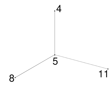
Figure 4: An example of a central-$3$-tree of a tree

If a different subset $Z$ is chosen at line $6$, we may get a different central-$3$-tree. This shows that a central-$k$-tree is not unique.

There might be central $k$-trees that do not arise from the algorithm as per McMorris’s and Reid’s  [8] remark:

There might be central $k$-trees that do not arise from the algorithm. For example, if $k=3$ and $T$ is the $7$-tree obtained by subdividing each edge of the complete bipartite graph $K(1,3)$, then each of three distinct subtrees of $T$ isomorphic to $K(1,2)$ are central 3-trees of $T$ arising from the algorithm. However, each of the three subtrees of order of order $3$ consisting of $2$-path starting from an end-node of $T$ is a central $3$-tree of $T$ as well. Line $6$ in the algorithm could be altered to allow $Z$ to be any $(k-|V(T(i)|)$-subset of $V(T)$ so that $T[U]$ is a $k$-tree, and all central $k$-trees would be produced by all such choices. The restriction of $Z$ to nodes in $L(i-1)$ in line $6$ insures that $T[U]$ is a subtree.

McMorris and Reid also give a proposition which states that for any integers $n$ and $k$, where $n\geq k\geq 1$, every $k$-tree is a central $k$-tree for some $n$-tree.

3 Central Forests

Let $k$ be the order of the subtrees of the tree $T$, and $\mathbb{F}_{T,m}$ the set of all forests in $T$ of $m$ subtrees each.

Definition 3.1.

The eccentricity of a single forest $F\in\mathbb{F}_{T,m}$ is given by:

$$e_{m}(F)\ \triangleq\ \mathrm{max}\ d(x,F),\forall x\in V(T).$$

Then the central forests of $T$ can be given by:

$$C(T;m,k)\ \triangleq\ \{F\ |\ e_{m}(F)\leq e_{m}(F^{\prime}),\ \forall F^{\prime}\in\mathbb{F}_{T,m}\}.$$

A single forest $F$ is a set of nodes, these nodes are divided into $m$ subtrees each of order $k$. The $e_{m}(F)$ calculates the eccentricity of forest $F$, i.e., the maximum distance between a node in $T-F$ and its nearest node in $F$.

Here, $C(T;m,k)$ denotes the central forest of $m$ subtrees of tree $T$ with each subtree being of order $k$. The central forest is defined as the forest $F$ in $\mathbb{F}_{T,m}$ such that $F$ has minimum of maximum distance between a node in $T-F$ and its nearest node in $F$, among all the forests $F^{\prime}$ in $\mathbb{F}_{T,m}$ i.e $e_{m}(F)\leq e_{m}(F^{\prime})$. Of course, $F$ need not be unique.

Remark 3.2.

Note that for the definition of $C(T;m,k)$ to be meaningful, we need to impose the restriction:

$$mk\leq|V(T)|.$$

The reason for this is that in a central forest, there are $m$ subtrees and order of each subtree is $k$. Hence, the total number of nodes in central forest is $m\times k$. Obviously, the number of nodes in central forest cannot exceed the number of nodes in $T$. So $mk\leq|V(T)|.$

Figure 5 gives an example of a tree with a central forest, specifically, $C(T;2,3)$. There are $2$ subtrees of order $3$ that make the central forest, i.e. $m=2$ and $k=3$. The nodes $3,4,5$ and $12,13,14$ make up the two subtrees which minimizes the maximum distance between a node in $\{1,2,6,7,8,9,10,11,15,16\}$ and its nearest node in $\{3,4,5,12,13,14\}$. The subtrees are surrounded by ovals for clarity.

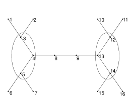
Figure 5: An example of a central forest.

Proposition 3.3.

The $m$-center is a special case of a central forest $C(T;m,k)$ for tree $T$, i.e., a $C(T;m,1)$ is equivalent to an $m$-center of tree $T$.

Proof.

As per Definition 3.1,

$$C(T;m,k)\ \triangleq\ \{F\ |\ e_{m}(F)\leq e_{m}(F^{\prime}),\ \forall F^{\prime}\in\mathbb{F}_{T,m}\}.$$

$F$ is a collection of $m$ subtrees of $T$. If $F$ is a central forest, then the eccentricity of subtrees of $F$ is minimum among all other possible sets of $m$-subtrees of tree $T$.

If the order of each subtree is $1$, then the set $X$ of these $m$ nodes makes the central forest $F$ and we have

$$C(T;m,k)\ \triangleq\ \{X\ |\ e(X)\leq e(Y),\ \forall\,Y\subseteq V(T),|Y|=m\}$$

By Definition 2.3, this is the $m$-center of tree $T$. ∎

Proposition 3.4.

The central-$k$-tree is a special case of central forest $C(T;m,k)$ for tree $T$, i.e. $C(T;1,k)$ is equivalent to the central-$k$-tree of tree $T$.

Proof.

As per Definition 3.1,

$$C(T;m,k)\ \triangleq\ \{F\ |\ e_{m}(F)\leq e_{m}(F^{\prime}),\ \forall F^{\prime}\in\mathbb{F}_{T,m}\}.$$

The central forest $F$ is a collection of $m$ subtrees of $T$, each subtree of order $k$. If $F$ is a central forest, then the eccentricity of subtrees of $F$ is minimum among all other possible sets of $m$-subtrees of tree $T$.

If there is only one subtree $W$ in $F$ of order $k$, then this subtree makes up the central forest and we have

$$C(T;m,k)\ \triangleq\ \{W\ |\ e_{m}(W)\leq e_{m}(W^{\prime}),\ \forall W^{\prime}\in\mathbb{F}_{T,m}\}.$$

By Definition 2.5, this is a central-$k$-tree in tree $T$.

∎

Observation 3.5.

The definition of a central forest is a generalization of the $m$-center and the central-$k$-tree.

3.1 Types of Subtrees in the Central Forest

There is only one type of tree of order 2, and only one of order 3, so $C(T;m,2)$ and $C(T;m,3)$ do not split into cases implied by the types of trees of those orders. In general, however, it is possible to have multiple sub-cases for $C(T;m,k)$. For instance, since there are two types of trees of order 4 (Figure 6), there are three possible cases for $C(T;m,4)$ (those containing subtrees of the first kind, those containing subtrees of the second kind, and those containing both kinds). In general, $C(T;m,k)$ is the union of the various sub-cases, some of which may be empty. The number of nonisomorphic trees of order $k=1,2,3,\ldots$ are $1,1,1,2,3,6,11,23,47,106,235,551,1301,$ $3159,\ldots$. The generating function for this sequence is

$$A(x)=1+T(x)-\frac{T^{2}(x)}{2}+\frac{T(x^{2})}{2}$$

where

$$T(x)=x+x^{2}+2x^{3}+4x^{4}+\ldots$$

satisfies

$$T(x)=x\exp(T(x)+\frac{T(x^{2})}{2}+\frac{T(x^{3})}{3}+\frac{T(x^{4})}{4}+\ldots)$$

as shown by Sloane [20] and the references therein.

Remark 3.6.

If $x$ is the number of nonisomorphic trees of order $k$, then the maximum number of possible combinations of different types of subtrees for central forest $C(T;m,k)$ is $x^{m}$.

Each subtree can be of one of the $x$ types of nonisomorphic trees. There are total $m$ subtrees in a central forest. So the maximum number of combinations of different types of subtrees for a central forest $C(T;m,k)$ is $x^{m}$.

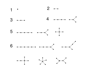
Figure 6: Nonisomorphic trees of order $1,2,3,4,5,6$

3.2 Properties of Central Forests in Trees

Observation 3.7.

The $1$-centers of the members of $C(T;m,k)$, do not necessarily consist of $m$-center of $T$,$\forall m,1\leq m\leq\lfloor\frac{|V(T)|}{k}\rfloor$.

We can show this with the help of an example of a $C(T;m,k)$. Consider a tree $T$ as shown in Figure 7, with small ovals around the nodes $2$ and $5$ indicating that these two nodes are $2$-centers of the tree $T$. In this figure the big ovals around the nodes represent the $2$ subtrees of order $4$ for $C(T;2,4)$. If we prune these subtrees, we get the node $6$ as one of the $1$-center, which is not originally a node in the $m$-center of the tree $T$. Therefore, the example clearly shows that $1$-centers of the members of $C(T;m,k)$, do not necessarily consist of $m$-center of $T$.

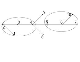
Figure 7: A central forest $C(T;2,4)$

Theorem 3.8.

Every $C(T;m,k)$ contains a $C(T;m,k-1),\ \forall m,\ 1\leq m\leq\lfloor\frac{|V(T)|}{k}\rfloor$.

Proof.

If we prune any tree of order $n$ to a tree of order $k$, we get a central-$k$-tree $W$, and by Definition 2.5 we have

$$\mathrm{Central}--k--\mathrm{tree}(T)\ \triangleq\ \{W\ |\ e(W)\leq e(W^{\prime}),\ \forall W^{\prime}\in W_{T,k},k\leq n\}.$$

As in Definition 2.5, $W_{T,k}$ is all subtrees of $T$ of order $k$. Now, if we prune $W$ to a tree $W^{\prime}$ of order $k-1$, the eccentricity of $W^{\prime}$ will also be minimum.

Thus, if we prune each member of $C(T;m,k)$ to subtrees of order $k-1$, we get all the members with minimum eccentricity. That is

$$C(T;m,k-1)\ \triangleq\ \{F\ |\ e_{m}(F)\leq e_{m}(F^{\prime}),\ \forall F^{\prime}\in\mathbb{F}_{T,m}\}.$$

This above equation is the definition of $C(T;m,k-1)$. Hence, every $C(T;m,k)$ contains a $C(T;m,k-1)$. ∎

Theorem 3.9.

All nodes of any $m$-center are part of members of some $C(T;m,k)$ of tree $T$, $\forall m,1\leq m\leq\lfloor\frac{|V(T)|}{k}\rfloor$.

Proof.

We prove this theorem by induction on $k$.

Base case: For $k=1$, the $m$ subtrees have only one node each. Then by Proposition 3.3, the members of $C(T;m,1)$ contain an $m$-center.

Inductive step: Let members of $C(T;m,k-1)$ contain an $m$-center of tree $T$. By this assumption, the $m$ members of $C(T;m,k-1)$ contain $m$-center, and by Theorem 3.8, every $C(T;m,k)$ contains a $C(T;m,k-1)$. Therefore, the members of $C(T;m,k)$ also contain $m$-center of tree $T$. ∎

3.3 The Upper Bound on the Order of Subtrees in a Central Forest

By Remark 3.2, we have a bound $mk$ $\leq$ $|V|$ that implies $k$ $\leq$ $\frac{|V|}{m}$. But this is a very loose bound as the bound on $k$ depend on the topology of the tree $T$.

Figure 8: A tree with adjacent nodes forming the $m$-center.

Remark 3.10.

When all the nodes of the $m$-center are adjacent to each other, the upper bound on $k$ can be obtained by pruning the edges connecting the nodes of $m$-center. This pruning of edges give us $m$ subtrees. In central forest, each subtree should be of same order. Therefore, the subtree with minimum number of nodes decide the order for all subtrees in central forest. And that is the upper bound on $k$.

An example tree where the nodes of the $m$-center are adjacent to each other is shown in Figure 8. In this figure the $5$-center is $\{a,b,c,d,e\}$, as shown by small ovals around the nodes. By Remark 3.10, if we prune the edges connecting this $5$-center, $d$ has minimum number of nodes ($4$) in its subtree. So the upper bound on $k$ is $4$.

But when the nodes of the $m$-center are not adjacent, finding the upper bound on $k$ is very difficult as it depends on the topology of the tree. In Section 4, we give an algorithm for constructing a central forest. This algorithm gives us the upper bound on $k$ when a central forest of $m$ subtrees, for the required value of $k$ is not possible.

4 An Algorithm CF to Construct a Central Forest

Given the topology of the tree $T$, we present an algorithm CF to construct the central forest $C(T;m,k)$ as defined in Section 3. The strategy followed by this algorithm is to divide the nodes of $T$ into $m$ subtrees such that the nodes are assigned to their nearest node in $m$-center.

The number of nodes in these subtrees may differ as per the topology of the tree $T$. There are two cases to consider, first when $k$ (the order of each subtree in the central forest) is less than or equal to the number of nodes in each of the $m$ subtrees. Second, when for one or more subtrees, $k$ is greater than the number of nodes present in those subtrees.

In the first case, we simply use the pruning algorithm given by McMorris and Reid  [8] to get a central-$k$-subtree for all the $m$ subtrees. These central-$k$-subtrees for all subtrees give us the central forest $C(T;m,k)$ in tree $T$.

In the second case, we try to extend all the subtrees with less nodes than $k$, by taking nodes from the neighboring subtrees. The neighbor subtree can itself take nodes from its neighbors, and so on. In this way, the second case is converted to the first. While taking nodes from other subtrees, the nodes that give the minimum increases in eccentricity of all subtrees are chosen. But if one or more subtrees cannot be extended to contain $k$ nodes, the CF algorithm outputs the minimum of number of nodes in a subtree among all subtrees, as the maximum order of the subtrees for which a central forest is possible.

Algorithm 2 builds the $m$ subtrees around the $m$-center by assigning each node to its nearest node in $m$-center. Algorithm 3 is used to extend one or more subtrees, if required. Pruning of subtrees, to get subtrees of order $k$, is done using Algorithm 4. The Algorithm 5 is the main algorithm which uses above said algorithms and outputs either the central forest or the maximum value of $k$ for which central forest of $m$ subtrees is possible for tree $T$.

4.1 Notation Used in Algorithms

• The set $V(T)$ is the set of nodes in tree $T$. The number of subtrees in the central forest is denoted by $m$. The order of each subtree in the central forest is $k$.

• The set $V_{m}$ holds all the nodes that make the $m$-center. In $V_{m}$ all the nodes of the $m$-center are indexed as per their occurrence.

• The two-dimensional matrix $ST$ contains all the nodes in the tree $T$ which are not a part of the set $V_{m}$. All nodes are assigned to the nearest node in the $m$-center. Each row of matrix $ST$ holds one of the nodes in $m$-center and all the nodes assigned to that node of $m$-center. The nodes of the $m$-center in $ST$ matrix appear in the order as in set $V_{m}$. The number of nodes in each row of $ST$ can be different, as it depends on how many nodes are assigned to each node of the $m$-center. If two or more nodes of the $m$-center are at equal distance from a node, then that node is made to wait till end and then it is assigned to the node of $m$-center which has lesser number of nodes in its corresponding row in matrix $ST$. If two or more nodes of the $m$-center have equal number of nodes in their corresponding row in the matrix $ST$, then the node is assigned to the node of $m$-center with lower value of index in set $V_{m}$.

• The one-dimensional matrix $H$ holds all nodes except the nodes of $m$-center.

• The two-dimensional matrix $u[r]$ holds the indices of all the nodes of the $m$-center that are at equal distance from node $r$.

• The one-dimensional matrix $z[l]$ holds the number of nodes in the $l^{th}$ row of $ST$, i.e. $ST[l]$.

• The $x[r]$ is a two dimensional matrix that stores the nodes that has to be removed from $ST[r]$ in order to remove $v$ as they are reachable via $v$ only, for nodes in $ST[r]$. $|x[r]|$ is the number of nodes in $x[r]$ . If not set, $|x[r]|$ holds value $0$.

• The one-dimensional matrix $d[r]$ holds the number of nodes left in $ST[r]$ when $|x[r]|$ nodes are taken out.

• The one-dimensional matrix $n[r]$ holds the number of nodes returned by ExtendST algorithm.

• The variable $color[v]$ holds either color ‘$White$’ or ‘$Gray$’. Initially all the nodes have ‘$White$’ color.

• The three dimensional matrix $B$, is used to store all the $ST$s that is produced by the algorithm.

• $C$ is a two-dimensional matrix which stores one row of $ST$ matrix at a time and keeps changing as the algorithm proceeds.

• $L$ is a two-dimensional matrix which holds the end nodes of $C$ at various stages.

• The set $X$ is any subset of $L(i)$ which has $k-|V(C)|$ nodes, where $i$ is the index of the row of the $L$ matrix.

• $U$ is a two-dimensional matrix, each row of which holds subtrees of order $k$, that collectively form the central forest.

• The two-dimensional matrix $A$ contains $m$ rows and $k$ columns. Each row of this matrix represents one of the $m$ subtrees of order $k$. In other words, $A$ holds the central forest $C(T;m,k)$ of $T$.

• The ExtractMin($r,V_{m}$) function returns the distance between the node $r$ and the nearest node in $V_{m}$.

• The function ExtractMinNum($r,u[r]$) returns the minimum number of nodes among the rows of $ST$ belonging to row $u[r]$.

• The function ExtractMinNumRow($r,u[r]$) returns the $ST$ row that has minimum number of nodes among the rows of $ST$ belonging to row $u[r]$. If two or more rows have minimum number of nodes, then the row with lower index value is returned.

• The NodesToBeRemoved($r,v$) is a function that returns the nodes that are reachable for any node in $ST[r]$, only through $v$, including $v$.

• The function AddRemoveNodes($x[r]$, $ST[l]$, $ST[r]$) adds, the nodes in matrix $x[r]$, from the $r^{th}$ row to the $l^{th}$ row of the $ST$ matrix.

• The function Store($ST,B$) stores the $ST$ in $B$.

• The function GetSTMinEccentricity($B$), returns the $ST$ that fulfills the requirement with minimum increase of eccentricity among all the $ST$s stored in $B$. If no $ST$ stored in $B$ fulfills the requirement, then the $ST$ that adds maximum number of nodes is returned.

• The function GetNodesAdded($ST,y$) returns the number of nodes added in $y^{th}$ row of $ST$.

• The function GetSTRow($v$) returns the index of the row of $ST$ which has $v$ node.

• The function GetMinSTRow($ST$) returns the index of row of $ST$ which has minimum number of nodes.

• The function ExtractMinNodes($ST$) extracts the minimum number of nodes among all the rows of $ST$.

• The function GetEndNodes($C$) returns the nodes that are end nodes in subtree $C$.

• The function GetSubset($L(i)$,$j$) returns one of the possible subsets of order $j$ from the $i^{th}$ row of matrix $L$.

4.2 Algorithms

Firstly, we present the algorithms used by the main CF algorithm. These algorithms build the $m$ subtrees ($ST$ matrix), extend subtree ($ST$ matrix row) and prune the $m$ subtrees to get subtrees of order $k$, respectively.

4.2.1 Algorithm $2$: Building the $ST$ Matrix

In the BuildST algorithm (Algorithm 2), we build the matrix $ST$ as defined in Section 4.1. The algorithm first gets minimum distance of a node $r$ and its nearest node in $m$-center. This distance is then compared with the distances of node $r$ and other nodes in $V_{m}$. The indices of all the nodes in $V_{m}$ which are at minimum distance from node $r$ are stored. If there is only one index stored for node $r$, then the node is added to the corresponding row of the $ST$. This is repeated for all the nodes which are in $V(T)$ but not in $V_{m}$. Then, at the end, for all those nodes which are at the same distance from more than $1$ nodes in $V_{m}$, the $ST$ row with minimum number of nodes among the indices stored for each node is chosen, and node is added to the selected row. If there are two or more $ST$ rows with minimum number of nodes, then the node is added to $ST$ row with lower index value.

In pseudocode for Algorithm 2, variable $min$ takes the distance between node $H[x]$ and the nearest node in $m$-center. Lines $7$–$9$ check, if $r$ is at equal distance from two or more node of the $m$-center in $V_{m}$. If $\mathbf{TRUE}$ then array $u[r]$ holds the indices of the corresponding nodes of the $m$-center, otherwise array $u[r]$ holds just the index of the nearest node in $m$-center.

In lines $10$–$14$, if $u[r]$ has only one index, the node $r$ is added to the $ST$ with index stored in $u[r]$, and $-1$ is added to $u[r]$ to indicate that this node has been added to some row of $ST$. The ‘while’ loop in line $4$ repeats this for all nodes in $H$.

for $i$ $\leftarrow$ $0$ to $m-1$ do $ST[i][0]$ $\leftarrow$ $V_{m}[i]$

$H$ $\leftarrow$ $V(T)-V_{m}$

$x$ $\leftarrow$ 0

while $H[x]$ $\neq$ $\emptyset$ do $min$ $\leftarrow$ ExtractMin($H[x],V_{m}$)

$h$ $\leftarrow$ $0$

for $i$ $\leftarrow$ $0$ to $m-1$ do if $min$ == $d(H[x],V_{m}[i])$ then $u[x][h++]$ $\leftarrow$ $i$

if $h==1$ then $v$ $\leftarrow$ $0$

while $ST[i][v]$ $\neq$ $\emptyset$ do $v\leftarrow v+1$

$ST[i][v]$ $\leftarrow$ $H[x]$

$u[x][h-1]$ $\leftarrow$ $-1$

$x\leftarrow x+1$

$x$ $\leftarrow$ $0$

while $H[x]$ $\neq$ $\emptyset$ do if $u[x][0]\neq$ $-1$ then $minNum$ $\leftarrow$ ExtractMinNum($u[x]$,$ST$)

$minNumRow$ $\leftarrow$ ExtractMinNumRow($u[x],ST$)

$ST[minNumRow][minNum]$ $\leftarrow$ $H[x]$

$x\leftarrow x+1$; return ($ST$)

Algorithm 2 BuildST($T$, $V_{m}$)

16

16

16

16

16

16

16

16

16

16

16

16

16

16

16

16

At line $18$, ‘if’ condition evaluates $\mathbf{TRUE}$ for those nodes which are at the same distance from more than one node of the $m$-center. Line $21$ adds any such node $r$ to the $ST$ row with minimum number of nodes among the $ST$ rows stored in row $u[r]$. If two nodes of the $m$-center have equal numbers of nodes, then node $r$ is added to the $ST$ row with lower index value.

Line $23$ returns the $ST$ matrix in which each row contains the nodes that are assigned to the first node (node in $m$-center) of the corresponding row.

4.2.2 Algorithm $3$: Extending a Row of the $ST$ Matrix

The ExtendST algorithm (Algorithm 3) extends one or more rows of $ST$ matrix by taking nodes from other rows of $ST$ matrix. A row $l$ can take nodes from its neighboring row i.e. a row which has the other end of an edge whose one end is in the row $l$. The Algorithm 3 takes one by one all the nodes in the $l^{th}$ row of $ST$, which we want to extend, and checks the adjacent nodes of each node. If the adjacent node is in another row then we explore that neighbor row. If the neighbor row has sufficient number of nodes, then we take nodes from that row and add to row $l$. Otherwise, the neighbor row itself can take nodes from its neighbor row and serve the requirement of row $l$. When the row $l$ has required number of nodes then algorithm stores the current $ST$ and mark the neighbors that are visited during this formation of $ST$. Algorithm again starts and in the same way, all the possible neighbors are explored and corresponding $ST$s are stored. In the end, the algorithm returns the $ST$ that fulfills the requirement with minimum increase of eccentricity among all the $ST$s stored. If no $ST$ fulfills the requirement, then $ST$ that adds maximum number of nodes is returned. Also the number of nodes added in row $l$ is returned.

The current $ST$ matrix, $l$, $y$ (index of $ST$ matrix row to extend), the value of $k$ and $OldST$ matrix are passed as input to this algorithm. Here, for the initial call of the algorithm $ST$ and $OldST$ are same. Also values of $l$ and $y$ are exactly same. It returns the new $ST$ and number of nodes added to row $y$ of $ST$.

In line $1$ of Algorithm 3, $z[l]$ takes the number of nodes in $ST[l]$. The ‘foreach’ loop in line $2$ runs for every node $u$ in $l^{th}$ row of $ST$, i.e. $ST[l]$. Second ‘foreach’ loop checks all the adjacent nodes of $u$.

If an adjacent node $v$ is not a part of $ST[l]$ and $color[v]$ is not ’$Gray$’, then $v$ belongs to one of neighbors of $ST[l]$ that is not explored yet. From lines $5$–$23$, the neighbor is explored to see if we can take nodes from this neighbor.

If node $v$ is in $V_{m}$, then this neighbor of $ST[l]$ cannot give any nodes, so we continue the ‘foreach’ loop of line $3$ with next adjacent node of $u$.

At line $5$, $stop$ is set to $\mathbf{FALSE}$ to indicate that some neighbor is explored in this loop. At line $10$, $d[r]$ is compared with $k$, if $d[r]\geq k$, then AddRemoveNodes function, adds nodes in $x[r]$ to $ST[l]$ and removes from $ST[r]$. At line $12$, the $color[v]$ is set to ‘$Gray$’.

At line $13$, if number of nodes added in $ST[l]$ minus number of nodes $ST[l]$ has to give, is greater than $k$, then $l$ is compared with $y$ to check whether it is the initial call or a recursive call. If it is the initial call to the algorithm, then control comes to line $25$. Otherwise, Algorithm 3 returns the number of nodes added in $ST[l]$. If the condition at line $13$ fails, then it continues the ‘foreach’ loop in line $3$ with other adjacent nodes of node $u$.

If the condition at line $10$ fails, i.e. $d[r]<k$, then we need to check if $ST[r]$ can be extended. In this case, we take some nodes from neighbors of $ST[r]$ and give some nodes to $ST[l]$ in order to fulfill the need of $ST[l]$. So basically we now extend $ST$ with changed row number of $ST$, hence a recursive call to Algorithm 3 is made as ExtendST($ST,r,k,y,OldST$).

The value it returns is taken in $n[r]$ and added to $d[r]$, and it checks whether $d[r]+n[r]\geq k$. If $\mathbf{TRUE}$ it adds the $x[r]$ nodes to $ST[l]$ and removes then from $ST[r]$. Next, we check $ST[l]$, if number of nodes in $ST[l]$ minus $x[l]$ is greater than $k$ then $l$ is compared with $y$ to check whether it is the initial call or a recursive call. If it is the initial call to algorithm, then control comes to line $25$. Otherwise, Algorithm 3 returns the number of nodes added in $ST[l]$. But, if the condition at line $20$ fails, then it continues the loop in line $3$ with other adjacent nodes of node $u$. If the condition at line $18$ fails, then $color[v]$ is set to $Gray$.

$z[l]\leftarrow|ST[l]|$

foreach $u\in ST[l]$ do foreach $v\in adj[u]$ do if $v\notin ST[l]$ and $color[v]\neq Gray$ then $stop\leftarrow\mathbf{FALSE}$

if $v\in V_{m}$ then continue

$r\leftarrow$ GetSTRow($v$)

$x[r]\leftarrow$ NodesToBeRemoved($v$)

$d[r]\leftarrow|ST[r]|-|x[r]|$

if $d[r]\geq k$ then AddRemoveNodes($x[r]$, $ST[l]$, $ST[r]$)

$color[v]\leftarrow Gray$

if $|ST[l]|-|x[l]|\geq k$ then if $l==y$ then Goto Line $25$

return ($|ST[l]|-z[l]$)

else  Continue

$n[r]\leftarrow$ ExtendST($ST,r,k,y,OldST$)

if $d[r]+n[r]\geq k$ then AddRemoveNodes($x[r]$, $ST[l]$, $ST[r]$)

if $ST[l]-|x[l]|\geq k$ then if $l==y$ then Goto Line $25$

return ($|ST[l]|-z[l]$)

else $color[v]\leftarrow Gray$

if $l\neq y$ then return ($|ST[l]|-z[l]$)

if $stop$ == $\mathbf{FALSE}$ then Store($ST,B$)

$ST\leftarrow OldST$

$stop\leftarrow\mathbf{TRUE}$

Goto Line $1$

$ST$ $\leftarrow$ GetSTMinEccentricity($B$)

$nodesAdded$ $\leftarrow$ GetNodesAdded($ST,y$)

return ($nodesAdded$)

Algorithm 3 ExtendST($ST$, $l$, $k$, $y$, $OldST$)

26

26

26

26

26

26

26

26

26

26

26

26

26

26

26

26

26

26

26

26

26

26

26

26

26

26

If all the nodes in $ST[l]$ have been checked and $ST[l]$ minus $x[l]$ is still less than $k$, then at line $24$, $l$ is compared with $y$ to check whether it is the initial call or a recursive call. If it is a recursive call, the number of nodes added to the $l^{th}$ row of $ST$ is returned. If it is a initial call to algorithm, then control comes to line $25$.

At line $25$, if $stop$ is $\mathbf{FALSE}$, then function Store($ST,B$) stores the current $ST$ in $B$, current $ST$ is replaced with $OldST$ and $stop$ is set to $\mathbf{FALSE}$. The algorithm starts with the initial call parameters to Algorithm 3 and this call generates a new $ST$. In this way we store all the possible $ST$s in $B$. When no neighbor is there to get nodes, the $ST$ which fulfills the required nodes with minimum possible increase of eccentricity is given as final output of the algorithm. This final $ST$ and number of nodes added in row $y$ are returned.

4.2.3 Algorithm $4$: Pruning the $ST$ Matrix Rows to Get a Central Forest

McMorris and Reid [8] have given a pruning algorithm for constructing central-$k$-tree in a given tree. We have to find $m$ central-$k$-subtrees for central forest $C(T;m,k)$. We have already divided the nodes into $m$ subtrees in $ST$. If we apply the central-$k$-tree algorithm to each subtree, we can get the central-$k$-subtree for each subtree.

The PruneST algorithm (Algorithm 4) prunes (removes) all the end-nodes of the tree and their corresponding edges in each step. After pruning, if the nodes in the resulting tree $T^{\prime}$ are less than or equal to $k$, then a subset of nodes from the nodes that are pruned in the last step is added to the nodes left in the tree $T^{\prime}$ and algorithm exits. The cardinality of this subset is $k-V(T^{\prime})$. Otherwise, if the number of nodes in the resulting tree is more than $k$, then prune all the end-nodes again. And this repeats for some definite number of steps.

foreach row $r$ of $ST$ do $C\leftarrow ST[r]$

$C(0)\leftarrow C$

$L(0)\leftarrow$ GetEndNodes($C$)

$i\leftarrow 1$

while $\mathbf{TRUE}$ do $C(i)\leftarrow C(i-1)/L(i-1)$

if $|V(C(i))|\leq k$ then $X\leftarrow$ GetSubset($L(i-1)$,$(k-|V(C(i))|)$)

$U[r]\leftarrow V(C(i))\cup X$

break

$L(i)\leftarrow$ GetEndNodes($C$)

$i\leftarrow i+1$

return ($U$)

Algorithm 4 PruneST($ST$, $k$)

10

10

10

10

10

10

10

10

10

10

The Algorithm 4 is taken from McMorris and Reid  [8] with some slight modifications. In Algorithm 4, every time line $2$ sets $C$ as the one of the subtrees(rows) of $ST$. $L(0)$ gets the end nodes of $C$. As in McMorris and Reid  [8], for a subset $L$ of the nodes of $C$, let $C/L$ denote the sub forest with node set $V(C)/L$ and edge set containing of all edges of $C$ incident with no node in $L$ i.e now $C/L$ contains all the nodes that are in $V(C)$ but not in $L$.

At line $8$, if the ‘if’ condition evaluates to $\mathbf{TRUE}$, $X$ takes any subset of $L(i-1)$ of order $k-|V(C(i)|$. The $U[r]$ ($U$ for $ST$ row $r$) is set to $V(C(i))$ $\cup$ $X$ and control comes out of infinite ‘while’ loop. Then, the ‘foreach’ loop of line $1$ starts with next row in $ST$.

But if the ‘if’ condition at line $8$ fails, then it continues in the ‘while’ loop. When all rows of $ST$ are done, the Algorithm 4 returns the matrix $U$.

Remark 4.1.

The forest $C(T;m,k)$ does not necessarily have unique subtrees, i.e. a $k$ node sub tree can be built by choosing a different set of nodes.

The justification for this remark is that central-$k$-tree of a tree is not unique. As shown in Section 2.4, we may get a different central-$k$-subtree using the same algorithm. Therefore, subtrees of $C(T;m,k)$ are also not unique.

4.2.4 Algorithm $5$: The Main Algorithm for Building a Central Forest

The CF algorithm (Algorithm 5) builds a central forest. The matrix $V_{m}$, tree $T$ and order of each subtree of central forest, $k$ are given as input to the algorithm. The value of $k$ should be less than or equal to the upper bound on $k$ as given by Remark  3.2. The output of this algorithm is the central forest with $m$ subtrees of order $k$ each. If central forest of order $k$ is not possible, then the algorithm outputs the maximum value of $k$ for which a central forest is possible.

$ST$ $\leftarrow$ BuildST($T$,$Vset_{m}[i]$)

$minNodes\leftarrow$ ExtractMinNodes(ST)

while $k>minNodes$ do foreach $u\in V(T)$ do $color[u]\leftarrow White$

$l\leftarrow$ GetMinSTRow()

$OldST\leftarrow ST$

$a\leftarrow$ ExtendST($ST,l,k,l,OldST$)

if $a==0$ then $ST\leftarrow OldST$

Output $minNodes$

Exit

$minNodes\leftarrow$ ExtractMinNodes(ST)

$A\leftarrow$ PruneST($ST$, $k$)

Algorithm 5 CF($T$, $V_{m}$, $k$)

11

11

11

11

11

11

11

11

11

11

11

Line $1$ calls the Algorithm 2 to build the matrix $ST$.

The $minNodes$ variable takes the minimum number of nodes in any row of matrix $ST$. At line $3$, the value of $minNodes$ is compared with the value of $k$. In the first case, when $k$ is less than or equal to $minNodes$, the condition at line $3$ fails and Algorithm 4 is called with parameters $ST$ and $k$ which returns the central forest.

But in the second case, when $k$ is greater than the $minNodes$, we need to extend that subtree (row) of $ST$, such that the number of nodes becomes equal or greater than the $k$. Also, there may be more than one subtrees (rows) that have nodes less than $k$, so at line $3$ ‘while’ loop repeats lines $4$–$13$ till any of the subtree (row) has less number of nodes than $k$.

Line $5$ sets the $color$ of each node in $V(T)$ as ‘$White$’. At line $8$, a call is made to Algorithm 3. The Algorithm 3 returns the number of nodes added to $l^{th}$ row of $ST$ and the new $ST$.

If the value of $a$ is $0$, no node can be added to $l^{th}$ row, thus the central forest for this value of $k$ is not possible. Line $10$ replaces new $ST$ with the $OldST$, i.e. $ST$ before the call to Algorithm 3. The value of $minNodes$ which is the maximum value for which the central forest is possible, is given as output and the Algorithm 5 exits. As mentioned in Section 3.3, this value is the required upper bound on the value of $k$ for tree $T$.

But if at line $8$, the value returned in $a$ is non-zero, then at line $13$ the function ExtractMinNodes(ST) extracts the minimum number of nodes among all the rows of new $ST$. The ‘while’ loop of line $3$ repeats till the value of $minNodes$ becomes equal to or less than $k$. When the condition at line $3$ fails, Algorithm 4 is called that returns a central forest in $A$ matrix.

4.3 An Example Demonstrating the CF Algorithm

We take a short example as shown in Figure 9 to demonstrate the working of Algorithm 5. In this example, we are constructing central forests stated as follows:

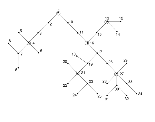
Figure 9: Example tree $T$

• $C(T;6,2)$ and

• $C(T;6,4)$

We are given
$V(T)=\{1,2,3,4,5,6,7,8,9,10,11,12,13,14,15,16,17,18,19,20,21,22,$
$23,24,25,26,27,28,29,30,31,32,33,34\}$
$V_{6}=\{1,4,13,16,21,27\}$

• For $C(T;6,2)$
  

  Algorithm 5 calls Algorithm 2 to build the $ST$ matrix. In Algorithm 2, $H$ = $\{2,3,5,6,7,8,9,10,11,12,14,15,17,18,19,20,22,23,24,25,$
  $26,28,29,30,31,$ $32,33,34\}$. Except node $15$, all the nodes have a unique nearest node in $V_{6}$. So all these nodes are directly added to the corresponding rows in $ST$ matrix and the $ST$ matrix is as shown in Table 1.

  At the end we check the array $u$ for non-zero values. Only the $u$ array of node $15$ holds the index $3$ and $4$. The number of nodes in row $3$ is equal to the number of nodes in row $4$, so node $15$ is added to the row with lower index value in $V_{6}$, i.e. row $3$. The final $ST$ matrix, as depicted in Table 2, is returned to the Algorithm 5.

  	1	2	3	4	5	6	7	8	9
  1	1	2	10
  2	4	3	5	6	7	8	9
  3	13	12	14
  4	16	11	17
  5	21	18	19	20	22	23	24	25
  6	27	26	28	29	30	31	32	33	34

  Table 1: Intermediate $ST$ matrix

  	1	2	3	4	5	6	7	8	9
  1	1	2	10
  2	4	3	5	6	7	8	9
  3	13	12	14	15
  4	16	11	17
  5	21	18	19	20	22	23	24	25
  6	27	26	28	29	30	31	32	33	34

  Table 2: $ST$ matrix

  Line $2$ of Algorithm 5 sets $minNodes=3$. The condition at line $3$ fails as $k=2$ here. So at line $14$ Algorithm 4 is called.

  In Algorithm 4, for the first time let $r$ be $1$ and $C$ gets $\{1,2,10\}$,$C(0)=\{1,2,10\}$ $L(0)=\{2,10\},i=1$. The condition at line $6$ is always true, so line $7$ sets $C(1)=C(0)/L(0)=\{1\}$. At line $8$, $|V(C(1)|=1$, is less than $k$ so $U[1]=\{1\}\cup X$, where $X$ can be $\{2\}$ or $\{10\}$. Let $X=\{2\}$, so $U[1]=\{1,2\}$. Similarly $U$ is calculated for every row of $ST$. Then the matrix $U$ is returned to Algorithm 5.

  At line $14$ of Algorithm 5, when the call to Algorithm 4 returns, $A$ holds the returned central forest.

  The central forest is shown in Figure 10. Here ovals are used to represent the nodes in each subtree of central forest. There are total $6$ ovals, each of which has $2$ nodes, thus we get $C(T;6,2)$.

  

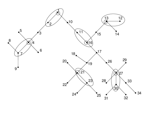
  Figure 10: A central forest $C(T;6,2)$ of example tree $T$

• For $C(T;6,4)$
  

  Line $1$ of Algorithm 5 builds $ST$ matrix in the same way as in case $1$.

  Line $2$ of Algorithm 5 sets $minNodes=3$. This time the condition at line $3$ is true. Lines $4$–$5$ set the $color$ of each node of $V(T)$ as ‘$White$’. Lines $6$ and $7$ set $l=1$ and $OldST=ST$. At line $8$, ExtendST($ST,1,4,1,OldST$) Algorithm 3 is called.

  In Algorithm 3, $z[1]=3$ as $ST[1]=\{1,2,10\}$. The ‘for’ loop in line $2$ starts with node $1$, ‘for’ loop in line $3$ checks nodes $2$ and $10$ (adjacent of $1$) but ‘if’ condition fails at line $4$. So now ‘for’ loop at line $2$ starts with next node in $ST[l]$ which is node $2$. Its adjacent node $3$ does not belong to $ST[1]$ and $color[3]$ is not ‘$Gray$’, so $stop$ is set to $\mathbf{FALSE}$. Also node $3$ does not belong to $V_{6}$ so lines $7-9$ set $r=2,x[2]=\{3\},d[2]=6$.

  The ‘if’ condition at line $10$ is true and node $3$ is added to $ST[1]$ and removed from $ST[2]$. The variable $color[3]$ is set to ‘$Gray$’. Condition at line $13$ is also true, so control comes to line $25$. Condition at line $25$ is $\mathbf{TRUE}$, so current $ST$ is stored in matrix $B$, current $ST$ is replaced with $OldST$, $stop$ is set to $\mathbf{TRUE}$ and control is transfered to line $1$.

  At line $1$ of Algorithm 3, $z[1]=3$ again as we have $ST[1]=\{1,2,10\}$. Proceeding in the same way, when the ‘for’ loop at line $2$ starts with node $2$. Its adjacent node $3$ does not belong to $ST[1]$ but $color[3]$ is ‘$Gray$’, so ‘for’ loop of line $2$ starts with next node in $ST[1]$, which is node $10$. Its adjacent node $11$ does not belong to $ST[1]$ and $color[11]$ is not ‘$Gray$’, so $stop$ is set to $\mathbf{FALSE}$. Also node $11$ does not belong to $V_{6}$ so lines $7-9$ set $r=4,x[4]=\{11\},d[4]=2$.

  Now condition at line $10$ fails and control comes to line $17$ where a recursive call is made to Algorithm 3 as ExtendST($ST,4,4,1,OldST$). This call starts the algorithm with $l=4$ and set $z[4]=3$. The ‘for’ loop in line $2$ checks all the nodes in $ST[4]$ one by one and for node $16$, ‘if’ condition of line $4$ evaluates $\mathbf{TRUE}$ as its adjacent node $15$ is neither in $ST[4]$ and nor ‘$Gray$’.

  So, $stop$ is set to $\mathbf{FALSE}$. Node $15$ also does not belong to $V_{6}$ so lines $7-9$ set $r=3,x[3]=\{15\},d[3]=3$.

  Now condition at line $10$ fails and control comes to line $17$ where a recursive call is made to Algorithm 3 as ExtendST($ST,3,4,1,OldST$). This call returns $0$ as $ST[3]$ does not have enough nodes to give and also it does not have any other neighbor.

  The condition at line $18$ fails as $n[3]$ is $0$ and $d[3]$ = $3$, so in else part $color[15]$ is set to ‘$Gray$’.

  The ‘foreach’ loop of line $3$ continues with other adjacent nodes of node $16$. There is no such node. So loop at line $2$ continues with next node in $ST[4]$, which is node $17$.

  Node $19$ is adjacent to node $17$ and it satisfy condition at line $4$ so $stop$ is set to $\mathbf{FALSE}$. The condition at line $6$ fails so lines $7$–$9$ set $r=5,x[5]=\{18,19\},d[5]=6$

  Now condition at line $10$ is true and nodes $18$ and $19$ are added to $ST[4]$ and removed from $ST[5]$. The variable $color[19]$ is set to ‘$Gray$’. Condition at line $13$ is $\mathbf{TRUE}$ but here $l$ is 4 which is not equal to $y$, so nodes added in $ST[4]$ is returned and $n[4]$ gets $2$.

  

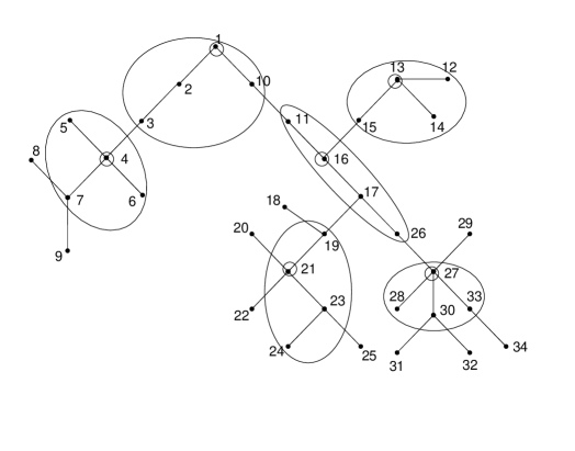
  Figure 11: A central forest $C(T;6,4)$ of example tree $T$

  At line $18$, $n[4]+d[4]$ = 4 is equal $k$ so node $11$ is added to $ST[1]$ and removed from $ST[4]$ and as $l=y$ the control is transferred to line $25$. The lines $26$–$29$, store current $ST$ in matrix $B$, replace current $ST$ with $OldST$, set $stop$ to $\mathbf{TRUE}$ and transfer to line $1$.

  Proceeding in the same way, we get $z[1]$ = $3$, for $u=10$ and $v=11$, $stop$ is set to $\mathbf{FALSE}$ and $r=4,x[4]=\{11\},d[4]=2$. As $d[4]$ is less than $k$ so a recursive call is made to Algorithm 3 as ExtendST($ST,4,4,1,OldST$).

  This call starts the algorithm with $l=4$ and set $z[4]=3$. For $u$ = $17$ and $v=26$, conditions at lines $4$ and $6$ evaluate $\mathbf{TRUE}$, so $stop$ is set to $\mathbf{FALSE}$ and $r=6,x[6]=\{26\},d[6]=8$.

  Now condition at line $10$ is true and node $26$ is added to $ST[4]$ and removed from $ST[6]$. $color[26]$ is set to ‘$Gray$’. Condition at line $13$ fails, the ‘foreach’ loop in line $3$ continues with other adjacent nodes of node $17$. But as there is no such node, the ‘foreach’ loop of $2$ checks next node in ST[4], but conditions at line $4$ and $6$ evaluate $\mathbf{FALSE}$ for every node. At line $24$, ‘if’ condition is true as $l=4$, so $color[11]$ is set to ‘$Gray$’. The lines $26$–$29$, store current $ST$ in matrix $B$, replace current $ST$ with $OldST$, set $stop$ to $\mathbf{TRUE}$ and transfer to line $1$.

  Here, $z[1]$ = $3$, condition at line $4$ evaluates $\mathbf{FALSE}$ for every node in $ST[1]$. At line $25$, ‘if’ condition fails as $stop$ is $\mathbf{TRUE}$. At line $30$, $ST$ gets the $ST$ that fulfills the requirement with minimum increase of eccentricity among all the $ST$s stored in $B$. If no $ST$ stored in $B$ that fulfills the requirement, then $ST$ that adds maximum number of nodes is returned. In our case, we choose $ST$ that adds node $3$ in $ST[1]$ from $ST[2]$. The $nodesAdded$ variable gets $1$ as the nodes added in row $1$ of $ST$ and returns to the main Algorithm 5.

  In Algorithm 5, condition at line $9$ fails, as $1$ node is added to $ST[l]$ and line $13$ sets $minNodes=3$. The ‘while’ loop at line $3$ evaluates $\mathbf{TRUE}$. Lines $4$–$5$ set the $color$ of each node of $V(T)$ as ‘$White$’. Line $11$ calls ExtendST($ST,4,4,4,OldST$). Proceeding in the same way as before the call to Algorithm 3 returns new $ST$ with node $26$ added to $ST[4]$ and removed from $ST[6]$.

  	1	2	3	4	5	6	7	8	9
  1	1	2	10	3
  2	4	3	5	6	7	8	9
  3	13	12	14	15
  4	16	11	17	26
  5	21	18	19	20	22	23	24	25
  6	27	26	28	29	30	31	32	33	34

  Table 3: Final $ST$ matrix

  The condition at line $9$ fails again and $minNodes$ gets $4$ which is equal to $k$, so condition at line $3$ fails. The final $ST$ matrix we got is shown in Figure 3.

  Then, control comes to line $14$ where Algorithm 4 is called. The Algorithm 4 works in the same way as explained for case $1$ and we get central forest in $A$.

  The central forest so obtained is shown in Figure 11. Here ovals are used to represent the nodes in each subtree of central forest. There are total $6$ ovals, each of which has $4$ nodes, thus we get $C(T;6,4)$.

4.4 Performance Analysis of the CF Algorithm

The running time of the CF algorithm depends upon the $ST$ returned by the Algorithm 2. If the nodes are assigned almost equally to all the nodes of the $m$-center then the Algorithm 5 runs very fast, but if the assignment of nodes is unbalanced, then it may take a long time depending on how large a value of $k$ is required. The time taken by Algorithm 5 is the sum of the running time of Algorithm 2, Algorithm 3, Algorithm 4 and the time taken by itself. In this section, we investigate how the Algorithm 5 performs. In any case, the Algorithm 2 costs $O(n(m+k))$ time, where $n$ is the number of nodes in the tree $T$. Algorithm 3 visit each node maximum of one or two times, so this takes $O(n)$ time. Algorithm 4 also takes $O(n)$ time. In Algorithm 5 other statements takes constant amount of time.

• Best Case Analysis
  

  The best case occurs when the required value of $k$ is less than or equal to the minimum number of nodes in any subtree of $ST$. This case mostly occurs when the $ST$ returns the subtree of almost the same order, i.e. the nodes are equally assigned to all the nodes of the $m$-center. Then, Algorithm 3 need not be called even once. So the running time of Algorithm 5 is as follows:

  $T(n)$ = Cost of Algorithm 2 + Cost of Algorithm 4 + Extra Cost of Algorithm 5

  $T(n)$ = $O(n(m+k))$ + $O(n)$ + $c$
  $T(n)$ = $O(n(m+k))$

• Worst Case Analysis
  

  Worst case occurs when $m-1$ subtrees of $ST$ returned by Algorithm 2 have less number of nodes in their subtrees than value of $k$. This can happen when one of the subtrees, which is in the center, has most of the nodes and all others are connected to the one in the center. The Algorithm 3 can be called once for all the $m-1$ subtrees and if for some row, number of nodes added is less than required, then Algorithm 3 is called once again for that row and this time Algorithm 3 returns $0$, so Algorithm 5 exits. Thus, the Algorithm 3 can be called maximum of $m$ times. Each of the call to Algorithm 3 costs $O(n)$. Therefore, $T(n)$ = Cost of Algorithm 2 + $m$ $\times$ Cost of Algorithm 3 + Cost of Algorithm 4 + Extra Cost of Algorithm 5

  $T(n)$ = $O(n(m+k))$ + $O(mn)$ + $O(n)$ + $c$
  $T(n)$ = $O(n(m+k))$

As we see, the worst-case behavior of the proposed algorithm is the same as its best case.

4.5 Proof of Correctness of the CF Algorithm

Remark 4.2.

Algorithm 2 builds an $ST$ matrix where each node is assigned to its nearest $m$-center node.

As shown in Minieka [10], an $m$-center set $X$ of a graph is any set of $m$ nodes, that minimizes the maximum distance from a node to its nearest node in $m$-center. In other words, the eccentricity of set $X$ is less than or equal to any possible set of cardinality $m$ of a graph. If such a set $X$ is given, each node can be arbitrarily assigned to its nearest node from the $m$-center. Thus all the nodes have minimum distance from the $m$-center. Such a set $X$ is given as input to Algorithm 2 and the algorithm assigns the nodes to their nearest nodes in $m$-center.

Lemma 4.3.

The re-arrangement of nodes in $ST$ rows by Algorithm 3 gives the rows in the new $ST$ matrix to minimize the distance from the $m$-center.

Proof.

All the nodes in the $ST$ matrix are so arranged by Algorithm 2 that their distances from the $m$-center are minimized. If we try to rearrange the nodes among the neighbors, the distances of the nodes may remain same (if a node is at equal distance from both the nodes of the $m$-center) or it may increase. We add nodes to a row $r$ only when the number of nodes in row $r$ is less than the value of $k$. The algorithm tries all the possible node(s) from neighbors that can be added to row $r$ and adds the node(s) which gives minimum increase of eccentricity for the $m$-center. So the overall eccentricity remains as small as possible. Obviously, there may be some increase in overall eccentricity but this cannot be avoided as we want number of nodes in row $r$ to be greater than or equal to $k$. Thus, Algorithm 3 gives the rows in new $ST$ with minimum increase in eccentricity. ∎

Lemma 4.4.

Algorithm 4 gives the $m$ central-$k$-subtrees for $m$ subtrees in $ST$.

Proof.

The nodes of $T$ are arranged in $ST$, each row of $ST$ is viewed as a separate subtree. McMorris and Reid [8] have given a proof that their algorithm outputs the central $k$-tree for any given tree. If we apply their algorithm for a subtree of $T$ then it gives us a central-$k$-subtree. In our Algorithm 4, we are using McMorris’s and Reid’s algorithm for each row of $ST$. So at the end we get $m$ central-$k$-subtrees for rows in $ST$. ∎

Lemma 4.5.

The $C(T;m,k)$ we get by building subtrees on $m$-center of tree $T$ is the same as a $C(T;m,k)$ we get by building subtrees on the $1$-centers of members of $C(T;m,k)$.

Proof.

We need to build $m$-subtrees in such a way that when we get a central-$k$-subtree of these $m$-subtrees, the eccentricity of each subtree is minimum. If we build our $m$-subtrees around the $1$-center of each member of $C(T;m,k)$ and we prune these subtrees to get central-$k$-subtrees, we get each member of $C(T;m,k)$. If we build subtrees around any other node from each members of $C(T;m,k)$, we get almost same subtrees as we get by choosing $1$-centers except some of the nodes may be assigned to the neighboring subtrees. By Theorem 3.9, the $m$-center of tree $T$, are part of members of some $C(T;m,k)$. Therefore, we know at least one node from each members of $C(T;m,k)$. We build $m$-subtrees around the $m$-center of tree $T$. As some of nodes may be assigned to the neighboring subtrees, so if we need more nodes in any subtree to build the subtree of order $k$, we take nodes from neighboring subtrees. Then, We apply pruning on these $m$-subtrees and get central-$k$-subtrees as members of $C(T;m,k)$. ∎

Theorem 4.6.

The Algorithm 5 gives either the central forest $C(T;m,k)$ for the tree $T$ with $m$ subtrees of order $k$ or outputs maximum possible order of a subtree and exits.

Proof.

The algorithm eventually terminates. Using Remark 4.2, Lemma 4.3, Lemma 4.4 and Lemma 4.5, it can be easily shown that Algorithm 4 outputs the forest with minimum eccentricity. Also, if Algorithm 3 returns $0$, the Algorithm 5 terminates and outputs the maximum possible value of $k$ for which central forest is possible. ∎

5 Conclusions and Further Work

In this paper we have introduced a new central structure in trees, which we call central forests in trees. $C(T;m,k)$ is a central forest of $m$ subtrees, each of order $k$, for tree $T$, which has minimum eccentricity among all the possible forests of this order for tree $T$. We have given an algorithm for constructing the central forests in trees. This algorithm is efficient as it computes the central forest in $O(n(m+k))$ time, where $n$ is the number of nodes in the tree $T$. The complete analysis and proof of correctness for the algorithm are also given in this paper. Our algorithm also computes a upper bound on the value of $k$ for which the central forest of $m$ subtrees is possible.

This work suggests the following possible extensions.

• Further Generalization

  • A further generalization is possible, if we allow that not all the subtrees in a central forest may be of like order.

    Then if $\mathbb{F}_{T,m}$ is the set of all forests in $T$ of $m$ subtrees each, and $\vec{\mathbf{a}}=(a_{0},a_{1},\ldots,a_{m-1})$ is a vector giving the orders of the $m$ subtrees with $a_{i}\neq 0$, then the eccentricity of a single forest is as given before, and a central forest $C(T;m,\vec{\mathbf{a}})$ is given by:

    $$C(T;m,\vec{\mathbf{a}})\ \triangleq\ \{F\ |\ e_{m}(F)\leq e_{m}(F^{\prime}),\ \forall F^{\prime}\in\mathbb{F}_{T,m}\}.$$

  • An interesting problem can be the study of forests $\Psi$ of subtrees (of variable orders and number) of a tree $T$ when the maximal allowable eccentricity $\delta$ is specified. One can give an algorithm that takes maximum allowable eccentricity and outputs the value of $m$ and $k$ for a $C(T;m,k)$. The problem is not well understood yet, it may be possible that no such algorithm exists and the problem posed is NP-hard.

  • Another potential area is to explore a similar extension to the concept of centroids, by defining a centroidal forest. Study the properties of centroidal forest and give a algorithm to construct such a forest in trees.

  • Another possible future work can be centrally use not more than $\sigma$ nodes and create not more than $\rho$ subtrees. That is, in central forest, there is a limit $\sigma$ on number of vertices that can be used in central forest. Also the number of subtrees ($m$) cannot be more than $\rho$ for a central forest. Under these restrictions, what is the minimum eccentricity possible for a central forest in a given tree?

• Further Work on the CF Algorithm

  • The algorithm we have given for constructing central forest is a centralized algorithm. A distributed algorithm, where nodes can decide whether they are part of a $C(T;m,k)$ or not, can be created.

  • The upper bound on the value of $k$ is given by the algorithm, we do not have a way to express the upper bound in terms of the degree of the tree, eccentricity, etc. Our upper bound depends on the algorithm output. A more generalized expression for upper bound on the value of $k$ for $m$ subtrees may be found.

  • We are assuming that an $m$-center of the tree is given and building our algorithm using this. One can think of an algorithm that does not require an $m$-center, or calculates this by itself.

References

- [1] S. C. Bruell, S. Ghosh, M. H. Karaata, and S. V. Pemmaraju, Self-stabilizing algorithms for finding centers and medians of trees, SIAM Journal on Computing, 29 (1999), pp. 600–614.
- [2] R. E. Burkard, H. Dollani, Y. Lin, and G. Rote, The obnoxious center problem on a tree, SIAM Journal on Discrete Mathematics, 14 (2001), pp. 498–509.
- [3] R. Chandrasekaran and A. Tamir, An algorithm for the continuous -center problem on a tree, SIAM Journal on Matrix Analysis and Applications, 1 (1980), pp. 370–375.
- [4] G. Y. Handler and P. B. Mirchandani, Location on Networks, MIT Press, Cambridge, MA, 1979.
- [5] S. M. Hedetniemi, E. J. Cockayne, and S. T. Hedetniemi, Linear algorithm for finding the Jordan center and path center of a tree, Transportation Science, 15 (1981), pp. 98–114.
- [6] C. Jordan, Sur les assemblages de lignes, J. Reine Angew Math, 70 (1869), pp. 185–190.
- [7] O. Kariv and S. L. Hakimi, An algorithmic approach to network location problems. I: The -centers, SIAM Journal on Applied Mathematics, 37 (1979), pp. 513–538.
- [8] F. R. McMorris and K. B. Reid, Central -trees in trees, Congressus Numerantium, 124 (1997), pp. 139–143.
- [9] N. Megiddo and A. Tamir, New results on the complexity of -center problems, SIAM Journal on Computing, 12 (1983), pp. 751–758.
- [10] E. Minieka, The -center problem, SIAM Review, 12 (1970), pp. 138–139.
- [11] , The optimal location of a path or tree in a tree network, Networks, 15 (1985), pp. 309–321.
- [12] P. B. Mirchandani and R. L. Francis, eds., Discrete Location Theory, Wiley Interscience, New York, 1990.
- [13] C. A. Morgan and P. J. Slater, A linear algorithm for the core of a tree, Journal of Algorithms, 1 (1980), pp. 247–258.
- [14] K. B. Reid, Centroids to centers in trees, Networks, 21 (1991), pp. 11–17.
- [15] P. J. Slater, Centers to centroids in graphs, Journal of Graph Theory, 2 (1978), pp. 209–222.
- [16] , Centrality of paths and vertices in a graph: Core and pits, The Theory of Applications of Graphs, (1981), pp. 529–542.
- [17] , The -nucleus of a graph, Networks, 11 (1981), pp. 233–242.
- [18] , On locating a facility to service areas within a network, Operations Research, 29 (1981), pp. 523–531.
- [19] , Locating central paths in a graph, Transportation Science, 16 (1982), pp. 1–18.
- [20] N. J. A. Sloane, Sequences a000055/m0791 number of trees with unlabeled nodes, The On-Line Encyclopedia of Integer Sequences.
- [21] A. Tamir, Improved complexity bounds for center location problems on networks by using dynamic data structures, SIAM Journal on Discrete Mathematics, 1 (1988), pp. 377–396.
- [22] , Obnoxious facility location on graphs, SIAM Journal on Discrete Mathematics, 4 (1988), pp. 550–567.
- [23] B. Zelinka, Medians and peripherians of trees, Arch. Math (Brno), 4 (1968), pp. 87–95.