Topological dynamics and dynamical scaling behavior of vortices in a two-dimensional XY model

Abstract

By using topological current theory we study the inner topological structure of vortices a two-dimensional (2D) XY model and find the topological current relating to the order parameter field. A scalar field, $\psi$, is introduced through the topological current theory. By solving the scalar field, the interaction energy of vortices in a 2D XY model is revisited. We study the dynamical evolution of vortices and present the branch conditions for generating, annihilating, crossing, splitting and merging of vortices. During the growth or annihilation of vortices, the dynamical scaling law of relevant length in a 2D XY model, $\xi(t)\propto(t-t^{*})^{1/z}$, is obtained in the neighborhood of the limit point, given the dynamic exponent $z=2$. This dynamical scaling behavior is consistent with renormalization group theory, numerical simulations, and experimental results. Furthermore, it is found that during the crossing, splitting and merging of vortices, the dynamical scaling law of relevant length is $\xi(t)\propto(t-t^{*})$. However, if vortices are at rest during splitting or merging, the dynamical scaling law of relevant length is a constat.

I INTRODUCTION

Vortices play an important role in understanding a variety of problems in physics. In the 1970s, Kosterlitz and Thouless constructed a detailed and complete theory of 2D systems Kt . The KT phase transition theory predicts that vortices pair unbinding will lead to a second-order transition in 2D systems, such as superfluid films, superconductors, and XY models two ; Dn . In a 2D XY model, there exist meta-stable states corresponding to vortices, which are closely bound in pairs below a critical temperature. Above the critical temperature, the paired vortices unbind and become free. Vortices in a 2D XY model disrupt the spin alignments even at large distances and correspond to singularities of the order-parameter field Cl .

In 2D XY model, vortices are topologically stable configurations. It is found that the high temperature disorder phase with an exponential correlation is a result of the formation of vortices. The critical temperature at which the KT transition occurs is, in fact, that at which vortex generation becomes thermodynamically favorable. At temperatures below this, the system has a power law correlation. In a low temperature phase, vortices appear in a small density of tightly bound dipole pairs. With an increase in temperature, vortex pairs dissociate and become free in the disorder phase. The evolution of vortices plays an important role in the KT transition of the 2D XY model.

There has been progress on the study of the defects associated with an n-component vector order parameter field, $\phi(\vec{r},t)$. For the scalar case (n=1), the defects are domain walls, which are points of the spatial dimensionality d=1, lines for d=2, planes for d=3, etc. More generally, for n=d, one has point defects. This leads to vortices for n=d=2. It is interesting to consider the appropriate form for the point defect densities when expressed in terms of the vector order parameter field. This has been carried out by Halperin Ha , and exploited by Liu and Mazenko LM ; however, their analyses are incomplete Duan00 . In a 2D system, a gauge field-theoretical formalism has been developed by Kleinert HK . Furthermore, the gauge theory of topological quantum melting in a $2+1$ dimensional Bose system was developed by Nussinov et al, and the superfluidity and superconductivity can arise in a strict quantum field-theoretical setting Z1 .

A topological field theory for topological defects has been developed by Duan et al Duan . By using the $\phi$-mapping method and topological current theory, the evolution of the topological defect that relates to singularities of the order-parameter field, such as the vortex in BEC Duan04 and superconductivity Duan05 , was studied. In this paper, we will discuss the topological quantization and evolution of vortex in two-dimensional XY model. We introduce a scalar field, $\psi$, through the topological current theory. By solving the scalar field, the Hamiltonian of the interaction of vortices in the 2D XY model is revisited.

More recently, the dynamical behavior of the 2D XY model following a quench of the temperature to below the KT critical temperature has been studied Br01 . During the quench of a dynamic 2D XY model, aging phenomena and dynamic scaling behavior become extremely important Bo . The assumption of dynamical scaling for the predicted asymptotic growth law the characteristic length, $\xi(t)\propto(t/lnt)^{1/2}$ Br02 , which is also characteristic of the spacing between defects. However, scaling violations were reported. According to an expansion in $\epsilon=4-d$ using standard field-theoretic renormalization group theory, it can be shown that the growing length is given as $\xi(t)\propto t^{1/z}$ for large t, where z is the critical exponent for equilibrium critical dynamics Jan . This standard theoretical approach also shows that the result $\xi(t)\propto t^{1/z}$ is independent of the initial conditions. However, this renormalization group method does not involve the effects of topological defects, such as vortices in the 2D XY model. In the recent work, it was shown that, for the specific case of the 2D XY model, $\xi(t)\propto(t/lnt)^{1/2}$ if free vortices are present, while $\xi(t)\propto t^{1/2}$ if there are no free vortices present in the initial state Brprl .

Through our topological current theory for the 2D XY model, the dynamic of vortices is studied, and the branch conditions for generating, annihilating, crossing, splitting and merging of vortices are given. During the growth or annihilation of vortices, the dynamical scaling law of relevant length in the 2D XY model, which is $\xi(t)\propto(t-t^{*})^{1/2}$, can be obtained in the neighborhood of the limit point. This indicates that vortices in the 2D XY model are the source of the scaling violations. This dynamical scaling behavior is consistent with numerical simulations LD and experimental results Pa . Furthermore, we have also found that during the crossing, splitting, and merging of vortices, the dynamical scaling law of relevant length in the 2D XY model, which is $\xi(t)\propto(t-t^{*})$. It has been shown that why the relevant length of vortices scales with time as $t^{-1/2}$ for small values of times and then deviate toward a linear dependence in nematic liquid-crystal experimental observations Pa2 . However, if vortices are at rest during splitting and merging, the dynamical scaling law of relevant length is $\xi=const$. Moreover, it is worthwhile to note that the dynamical scaling law of vortices, which was deduced from the topological current theory, only depends on topological properties of the order parameter field.

The organization of this paper is as follows. In Sec. II, we describe the 2D XY model and the $\phi$-mapping method, and topological current theory is discussed. The Hamiltonian of vortices in the 2D XY model is revisited in section III. The evolution of vortices and dynamical scaling discussed in section IV. Finally, in section V, we summarize our results.

II Topological Current in the 2D XY model

The 2D XY model is a system of spins confined to rotate in the plane of the lattice. The Hamiltonian of the system is give as:

$$H_{0}=-J\sum_{<ij>}\textbf{S}_{i}\textbf{S}_{j}=-J\sum_{<ij>}\cos(\theta_{i}-\theta_{j}),$$ (1)

where J is the strength of the nearest-neighbor interaction. $\theta_{i}$ denotes the angle of the spin on site i with respect to arbitrary polar direction in the 2D vector space containing spins.

By using the continuum limit, we can approximate $\cos(\theta_{i}-\theta_{j})$ by the first two terms $1-(\theta_{i}-\theta_{j})^{2}/2$ of the Taylor expansion. We can express partial derivatives through $\theta_{i}-\theta_{j}=\partial\theta$ for the two sites i and j. This leads to the continuum Hamiltonian:

$$H=H_{0}-E_{0}=\frac{J}{2}\int d\textbf{r}(\nabla\theta)^{2},$$ (2)

where $E_{0}=2JN$ is the energy of the completely aligned ground state of $N$ spins.

Kosterlitz and Thouless suggested that the disordering is caused by topological defects, such as vortices in two-dimensional XY model, which are characterized by a mapping from some loop $\Gamma$ in real space onto the order parameter space. For two-dimensional XY model, this implies

$$\oint d\theta=\oint\nabla\theta d\vec{s}=2\pi W,W=0,\pm 1,\ldots,n,$$ (3)

where $W$ is the winding number of the vortex. By introducing a 2D XY model, the local order parameter is defined as:

$$\Psi=\Psi_{0}e^{i\theta}=\phi^{1}+i\phi^{2}.$$ (4)

Quantized vortices are topological objects associated with topological properties of the order parameter $\Psi$. It is worth noting that the phase of the order parameter is undefined at the vortex core. In other words, vortices correspond to singularities of the order-parameter field. We define the unit vector field $\vec{n}$ as

$$n^{a}=\frac{\phi^{a}}{||\phi||},~{}||\phi||=\sqrt{\phi^{a}\phi^{a}},~{}a=1,2.$$ (5)

where $n^{a}n^{a}=1$. From the unit vector, $\vec{n}(x)$, we can construct a topological current of the order parameter field in the 2D XY model, which carries the topological information of $\vec{\phi}(x)$:

$$j^{k}=\frac{1}{2\pi}\epsilon^{ijk}\epsilon_{ab}\partial_{i}n^{a}\partial_{j}n^{b},\quad i,j,k=0,1,2.$$ (6)

We will see that this current does not vanish at the zero point of $\vec{\phi}(x)$ or the singularities of the unit field $\vec{n}(x)$. By using the 2D topological current theorem, Eq. (6) can be rewritten in the compact form;

$$j^{k}=\delta^{2}(\vec{\phi})J^{k}\left(\frac{\phi}{x}\right).$$ (7)

It is the important relation between the $\delta-$like topological current of vortices and the order parameter, $\Psi$, where $J^{k}(\phi/x)$ is the vector Jacobian of $\vec{\phi}$:

$$J^{k}\left(\frac{\phi}{x}\right)=\frac{1}{2}\epsilon^{ijk}\epsilon_{ab}\partial_{i}\phi^{a}\partial_{j}\phi^{b},$$ (8)

or

$$J^{0}\left(\frac{\phi}{x}\right) = \det\left(\begin{array}[]{cc}\partial_{x}\phi^{1}&\partial_{y}\phi^{1}\\ \partial_{x}\phi^{2}&\partial_{y}\phi^{2}\end{array}\right),$$ (11)

$$J^{1}\left(\frac{\phi}{x}\right) = \det\left(\begin{array}[]{cc}\partial_{y}\phi^{1}&\partial_{t}\phi^{1}\\ \partial_{y}\phi^{2}&\partial_{t}\phi^{2}\end{array}\right),$$ (14)

$$J^{2}\left(\frac{\phi}{x}\right) = \det\left(\begin{array}[]{cc}\partial_{t}\phi^{1}&\partial_{x}\phi^{1}\\ \partial_{t}\phi^{2}&\partial_{x}\phi^{2}\end{array}\right).$$ (17)

According to the implicit function theorem, the Jacobian’s determinant can be given as:

$$J^{0}\left(\frac{\phi}{x}\right)=J\left(\frac{\phi}{x}\right)\neq 0,$$ (18)

The solutions of the zero point of $\vec{\phi}(x)$ can be generally expressed as:

$$x=x_{l}(t),\quad y=y_{l}(t),\quad l=1,2,\ldots,N,$$ (19)

which represent $N$ zero points, $\vec{z_{l}}(t)$ (l=1,2,…,N), or a world line of $N$ vertices in space-time.

With the $\delta$-function theory, $\delta^{2}(\phi)$, can be expanded as:

$$\delta^{2}(\phi)=\sum_{l=1}^{N}\frac{\beta_{l}}{|J(\phi/x)_{z_{l}}|}\delta^{2}\left(\vec{r}-\vec{z_{l}}(t)\right)$$ (20)

where the positive integer, $\beta_{l}$, is called the Hopf index of map $x\rightarrow\vec{\phi}$. The meaning of $\beta_{l}$ is that when the point $\vec{r}$ covers the neighborhood of the zero, $\vec{z_{l}}$, once the vector field, $\vec{\phi}$, covers the corresponding region for $\beta_{l}$ times. Using the implicit function theorem and the definition of the vector Jacobian (Eq. 8), we can find the velocity of the $l$-th defect,

$$\vec{v_{l}} = \frac{d\vec{z_{l}}}{dt}=\left[\frac{\vec{J}(\phi/x)}{J(\phi/x)}\right]_{\vec{z_{l}}}$$

$$\vec{J}\left(\frac{\phi}{x}\right) = \left[J^{1}\big{(}\phi/x\big{)},J^{2}\left(\phi/x\right)\right]$$ (21)

The spatial and temporal components of the defect current, $j^{k}$, can be written as the form of the current and the density of a system of $N$ classical point particles moving in a $(2+1)$-dimensional space-time,

$$\vec{j}=\sum_{l=1}^{N}\beta_{l}\eta_{l}\vec{v_{l}}\delta^{2}(\vec{r}-\vec{z_{l}}(t))$$ (22)

$$j^{0}=\rho=\sum_{l=1}^{N}\beta_{l}\eta_{l}\delta^{2}(\vec{r}-\vec{z_{l}}(t))$$ (23)

where $\eta_{l}$ is the Brouwer degree,

$$\eta_{l}=\frac{J(\phi/x)}{|J(\phi/x)|}\bigg{|}_{\vec{z_{l}}}=\pm 1.$$ (24)

It can clearly be seen that Eq. (22) shows the movement of vertices. The topological charge of vertices in the 2D XY model are conserved:

$$\frac{\partial\rho}{\partial t}+\nabla\vec{j}=0.$$ (25)

In addition, there is a constraint of charge neutrality:

$$\int\rho d^{2}x=\frac{1}{2\pi}\sum_{l=1}^{N}\beta_{l}\eta_{l}=0,$$ (26)

which indicates that vortices in the 2D XY model appear in pairs.

III The Hamiltonian of vortices in the 2D XY model revisited

In analogy to the velocity field in a superfluid, the distortion field, $\vec{u}=\nabla\theta$, carries the topological information of vortices in the 2D XY model. By using Eq. (4) and (5), we can prove that

$$\vec{u}=\epsilon_{ab}n^{a}\nabla n^{b},$$

and the vorticity is given as:

$$\nabla\times\vec{u}=\textbf{e}_{i}(\epsilon^{ijk}\epsilon_{ab}\partial_{j}n^{a}\partial_{k}n^{b})$$ (27)

where $\textbf{e}_{k}(k=1,2,3)$ are the base vectors in the Cartesian coordinate system. Comparing Eq. (27) and Eq. (6), we conclude that

$$\nabla\times\vec{u}=2\pi j^{0}\textbf{z}.$$ (28)

Therefore, in the 2D XY model, the vorticity of distortion field, $\nabla\times\vec{u}$, can be expressed in terms of the topological current of the order parameter field. By comparing the $\delta-$like topological current Eq. (7) and Eq. (28), we have the important relation between vorticity and the order parameter field in the 2D XY model:

$$\nabla\times\vec{u}=2\pi\delta^{2}(\phi)J\left(\frac{\phi}{x}\right)\textbf{z},$$ (29)

From Eq. (29), we see that the vorticity of distortion field, $\nabla\times\vec{u}$, does not vanish at the zero points of $\Psi$. The location and direction of the $i$th vortex are determined by the $i$th singular point, $\vec{z_{l}}(t)$, and the vector Jacobian, $J(\phi/x)$, on $\vec{z_{l}}(t)$, respectively. In the absence of vorticity, there are no zero values of the order parameter field, $\delta^{2}(\phi)$ is zero, and Eq. (29) becomes:

$$\nabla\times\vec{u}_{0}=0,$$ (30)

which is the condition of irrotationality. Thus, Eq. (29) describes both the vortex-state and the irrotationality-state. To describe a collection of vortices at locations $\vec{z_{l}}(t)$, we substitute Eq. (23) into Eq. (28), leading to:

$$\nabla\times\vec{u}=2\pi\sum_{l=1}^{N}\beta_{l}\eta_{l}\delta^{2}(\vec{r}-\vec{z_{l}}(t))\textbf{z}.$$ (31)

It can be see that Eq. (31) represents N vortices that are charged with the topological charge, $W$. $W$ is $\beta_{l}\eta_{l}$, which describes the inner topological structure of the vortex. To find the solution for Eq. (31), we can introduce a harmonious scalar field, $\psi$ defining by:

$$\nabla^{2}\psi =\partial_{i}\partial_{j}\theta-\partial_{j}\partial_{i}\theta$$ (32)

$$=\epsilon^{ij}\epsilon_{ab}\partial_{i}n^{a}\partial_{j}n^{b}.$$

In the absence of a vortex in the 2D XY model, we can see that the condition, $\partial_{i}\partial_{j}\theta=\partial_{j}\partial_{i}\theta$, leads to $\nabla^{2}\psi=0$. Thus, the 2D distortion can be written as, $\vec{u}=\vec{u}_{0}-\nabla\times(\textbf{z}\psi)$, which contains two parts: the first part, $\vec{u}_{0}=\nabla\phi$, describe spin waves, while the second part is associated with vortices. By using 2D topological current theorem, it can be shown that:

$$\nabla^{2}\psi=2\pi\sum_{l=1}^{N}\beta_{l}\eta_{l}\delta^{2}(\vec{r}-\vec{z_{l}}(t)).$$ (33)

The scalar field, $\psi$, behaves like the potential due to a set of charged particles. The solution of Eq. (33) is given as:

$$\psi(x)=\sum_{l=1}\beta_{l}\eta_{l}ln(|\vec{r}-\vec{z_{l}}(t)|).$$ (34)

The continuum Hamiltonian of the vortices in Eq. (2) can be rewritten as:

$$H-\sum_{i}E_{ci}=\frac{J}{2}\int(\nabla\psi)^{2}d^{2}\textbf{x}=-\frac{J}{2}\int\psi\nabla^{2}\psi,d^{2}\textbf{x}$$ (35)

where $E_{ci}$ is the core energy of the vortex. Substituting Eq. (33) and (34) into the Hamiltonian (35), one can obtain:

$$\beta H=\beta E_{c}\sum_{i}W_{i}^{2}-\pi K\sum_{ij}W_{i}W_{j}ln(\vec{z_{i}}(t)-\vec{z_{j}}(t)),$$ (36)

which is identical to the Hamiltonian of a 2D Coulomb gas with point charges of charge $W_{i}=\beta_{i}\eta_{i}$. The constraint given by Eq. (26) is thus the constraint of charge neutrality.

IV The evolution of vortices in the 2D XY model

The zero point of the order parameter field, $\Psi$, which is associated with the locations of the core of vortices, plays an important role in describing the evolution of vortices in the 2D XY model. If the Jacobian determinant, $J^{0}(\phi/x)\neq 0$, we will have the isolated solution of the zeros of the order parameter field in $2+1$ dimensional space-time. But, when $J^{0}(\phi/x)=0$, the above results will change in some way and will lead to the branch process of vortices. We denote one of the vectors Jacobians at the zero points as $(t^{*},\vec{z_{l}})$. According to the values of the vector Jacobian at the zero points of the order parameter, there are usually two kinds of branch points, namely, the limit points and bifurcation points KU . Each kind corresponds to different cases of branch processes.

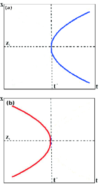
Figure 1: Generating and annihilating of vortices pairs. (a) The origin of two vortices. (b) Two vortices annihilate in collision at the limit point.

IV.1 The generation and annihilation of vortices

We explore what will happen to vortices at the limit point $(t^{*},\vec{z_{l}})$. The limit points are determined by

$$J^{0}\left.\left(\frac{\phi}{x}\right)\right|_{t^{*},\vec{z_{l}}}=0,\quad J^{1}\left.\left(\frac{\phi}{x}\right)\right|_{t^{*},\vec{z_{l}}}\neq 0$$ (37)

$$J^{0}\left.\left(\frac{\phi}{x}\right)\right|_{t^{*},\vec{z_{l}}}=0,\quad J^{2}\left.\left(\frac{\phi}{x}\right)\right|_{t^{*},\vec{z_{l}}}\neq 0.$$ (38)

Considering the condition given by Eq. (37) and making use of the implicit function theorem, the solution of the zero points of $\phi(x)$ in the neighborhood of the point ($t^{*},\vec{z_{l}}$) is given as:

$$t=t(x),\quad y=y(x),$$ (39)

where $t^{*}=t(z_{l}^{1})$. In this case, one can see that:

$$\left.\frac{dx}{dt}\right|_{(t^{*},\vec{z_{l}})}=\left.\frac{J^{1}(\phi/x)}{J(\phi/x)}\right|_{(t^{*},\vec{z_{l}})}=\infty,$$ (40)

or

$$\left.\frac{dt}{dx}\right|_{(t^{*},\vec{z_{l}}}=0.$$ (41)

The Taylor expansion of $t=t(x)$ at the limit points $(t^{*},\vec{z_{l}})$ is given as:

$$t-t^{*}=\left.\frac{1}{2}\frac{d^{2}t}{dx^{2}}\right|_{t^{*},\vec{z_{l}}}(x-z_{l}^{1})^{2},$$ (42)

which is a parabola in the x-t plane. From this equation, we can obtain two solutions $x_{1}(t)$ and $x_{2}(t)$, which give two branch solutions (world lines of the vortices). If

$$\left.\frac{d^{2}t}{dx^{2}}\right|_{(t^{*},\vec{z_{l}})}>0,$$

we have the branch solutions for $t>t^{*}$ which are related to the origin of a dipole pair. Otherwise, we have the branch solutions for $t<t^{*}$, which related to the annihilation of a dipole pair (Fig. 1).

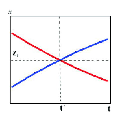
Figure 2: Two vortices collide with different directions of motion at the bifurcation point in $(2+1)$-dimensional space-time. Two world lines intersect with different directions at the bifurcation point; i.e., two vortices encounter at the bifurcation point.

Since the topological current is identically conserved, the topological charges of these two generated or annihilated vortices must be opposite of one another at the limit points, such as:

$$\beta_{1}\eta_{1}+\beta_{2}\eta_{2}=0.$$ (43)

This indicates that the vortices always generate and annihilate in pairs. From Eq. (42), one also obtains that the velocity of the vortices is infinite when they are annihilating, which agrees with the result introduced by Bray Bray . Furthermore, a new result can be obtained that shows that the velocity of the vortices is infinite when they are generating, which is gained only from the topology of the order parameter field. For a limit point, it is required that, $J^{1}(\phi/x)|_{t^{*},\vec{z_{l}}}\neq 0$. A bifurcation point, on the other hand, must satisfy a more complex condition. This case will be discussed in the following.

IV.2 Encountering, Splitting and Merging of vortices

Now, let us turn to consider the case in which the restrictions on the zero point $(t^{*},\vec{z_{l}})$ are given by:

$$J^{k}\left.\left(\frac{\phi}{x}\right)\right|_{(t^{*},\vec{z_{l}})}=0,\quad k=0,1,2,$$ (44)

which imply an important fact that the function relationship between t and x or y is not unique in the neighborhood of the bifurcation point $(t^{*},\vec{z_{l}})$. This fact is easily seen from

$$\frac{dx}{dt}=\left.\frac{J^{1}(\phi/x)}{J(\phi/x)}\right|_{t^{*},\vec{z_{l}}},~{}~{}\frac{dy}{dt}=\left.\frac{J^{2}(\phi/x)}{J(\phi/x)}\right|_{t^{*},\vec{z_{l}}},$$ (45)

which, under Eq. (44), directly shows the indefiniteness of the direction of the integral curve of Eq. (45) at $(t^{*},\vec{z_{l}})$. For this reason, the point $(t^{*},\vec{z_{l}})$ is called a bifurcation point of the orientation order parameter.

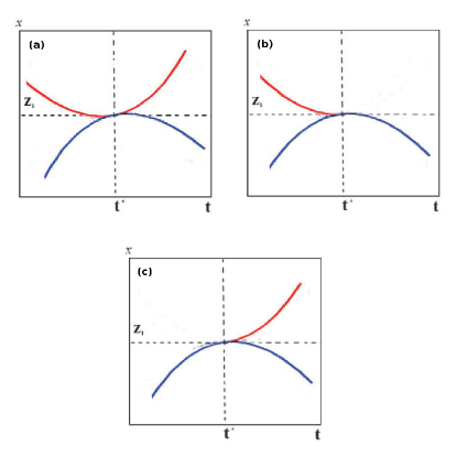
Figure 3: Vortices with the same direction of motion. (a) Two world lines tangentially contact; i.e., two vortices tangentially encounter at the bifurcation point. (b) Two world lines merge into one world line; i.e., two vortices merge into one vortex at the bifurcation point. (c) One world line resolves into two world lines; i.e., one vortex splits into two vortices at the bifurcation point.

As we know, at the bifurcation point, $(t^{*},\vec{z_{l}})$, the rank of the Jacobian matrix, $\left[\partial\phi/\partial\textbf{x}\right]$, is $1$ in the 2D vector order parameter. With the aim of finding the different directions of all branch curves at the bifurcation point, we assume:

$$\left.\frac{\partial\phi^{1}}{\partial y}\right|_{t^{*},\vec{z_{l}}}\neq 0.$$ (46)

From the implicit function theorem, there is one function relation:

$$y=f(x,t).$$ (47)

According to the $\phi$-mapping theory, the Taylor expansion of the solution of the zeros of the order parameter field in the neighborhood of $(t^{*},\vec{z_{l}})$ can be expressed as: Duan

$$A(x-z_{l}^{1})^{2}+2B(x-z_{l}^{1})(t-t^{*})+C(t-t^{*})^{2}+\cdots=0,$$ (48)

which leads to

$$A\left(\frac{dx}{dt}\right)^{2}+2B\frac{dx}{dt}+C=0,$$ (49)

and

$$C\left(\frac{dt}{dx}\right)^{2}+2B\frac{dt}{dx}+A=0,$$ (50)

where A, B, and C are constants determined by the order parameter. The solutions of Eq. (49) or Eq. (50) give different directions for the branch curves (world line of the vortices) at the bifurcation point. There are four possible cases which demonstrate the physical meaning of the bifurcation points.

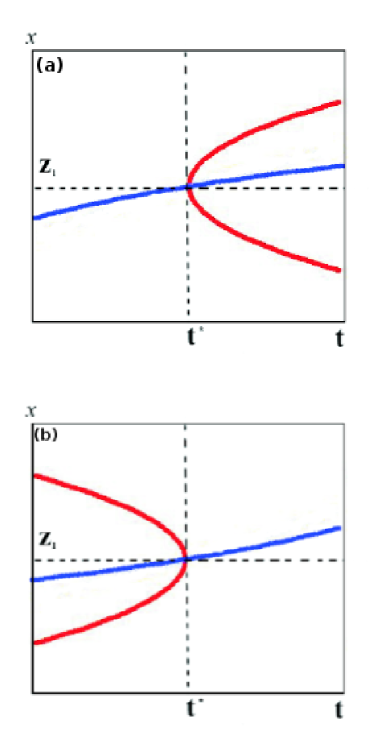
Figure 4: Two important cases of Eq. (53). (a) One world line resolves into three world lines; i.e., one vortex resolves into three vortices at the bifurcation point. (b) Three world lines merge into one world line; i.e., three vortices merge into one vortex at the bifurcation point.

Case 1 $(A\neq 0)$: For $\Delta=4(B^{2}-AC)>0$, from Eq. (49) we get two different motion directions of the core of the vortex given as:

$$\left.\frac{dx}{dt}\right|_{1,2}=\frac{-B\pm\sqrt{B^{2}-AC}}{A},$$ (51)

which is shown in Fig. 2, where two world lines of two vortices intersect with different directions at the bifurcation point. This shows that two vortices encounter and then depart at the bifurcation point.

Case 2 $(A\neq 0)$: For $\Delta=4(B^{2}-AC)=0$, form Eq. (49), we obtain only one motion direction of the core of the vortex given as:

$$\left.\frac{dx}{dt}\right|_{1,2}=-\frac{B}{A},$$ (52)

which includes three important cases (Fig. 3). These three cases are: (i) Two world lines tangentially contact; i.e., two vortices tangentially encounter at the bifurcation point. (ii) Two world lines merge into one world line; i.e., two vortices merge into one vortex at the bifurcation point. (iii) One world line resolves into two world lines; i.e., one vortex splits into two vortices at the bifurcation point.

Case 3 $(A=0,C\neq 0)$: For $\Delta=4(B^{2}-AC)=0$, from Eq.(49) we have:

$$\left.\frac{dt}{dx}\right|_{1,2}=\frac{-B\pm\sqrt{B^{2}-AC}}{C}=0,~{}-\frac{2B}{C}.$$ (53)

There are two important cases (Fig. 4): (i) One world line resolves into three world lines; i.e., one vortex splits into three vortices at the bifurcation point. (ii) Three world line merge into one world line; i.e., three vortices merge into one vortex at the bifurcation point.

Case 4 (A=C=0): Equations (49) and (50) give respectively:

$$\frac{dx}{dt}=0,\quad\frac{dt}{dx}=0.$$ (54)

This case shows that two world lines intersect normally at the bifurcation point, which is similar to case 3. It is no surprise that both parts of Eq. (54) are correct because they give the slope coefficients of two different curves at the same point $(t^{*},\vec{z_{l}})$.

The remaining components of $dy/dt$ can be calculated from a function relation of Eq. (47):

$$\frac{dy}{dt}=\frac{\partial f}{\partial x}\frac{\partial x}{\partial t}+\frac{\partial f}{\partial t}.$$ (55)

The above solutions reveal the evolution of the vortices. The topological structure of the vortices is detailed in the neighborhood of the bifurcation points of the order parameter field. Besides the encountering of vortices, i.e., two vortices encountered at and then depart from the bifurcation point along different branch curves (Fig. 2 and Fig. 3(a)), splitting and merging of vortices are also included. When multicharged vortices pass the bifurcation point, it may split into several vortices along different branch curves (Fig. 3(c), Fig. 4(a)). On the other hand, several vortices can merge into one vortex at the bifurcation point (Fig. 3(b), Fig. 4(c)). As before, since the topological current of the vortices is identically conserved, the sum of topological charges of the final vortices must be equal to that of the initial vortices at the bifurcation point, which is given as (for fixed l):

$$\sum_{f}\beta_{lf}\eta_{lf}=\sum_{i}\beta_{li}\eta_{li}.$$ (56)

This indicates that vortices with a higher value of Burgers vector can evolve to the lower value of Burgers vector, or that vortices with a lower value of Burgers vector can evolve to a the higher value of Burgers vector through the bifurcation process. Furthermore, we see that the generation, annihilation, and bifurcation of vortices are not gradual changes, but that they start at a critical value of a parameter, i.e., a sudden change. It is important to note that further bifurcations are possible during the evolution of vortices besides the cases studied in this work. It is necessary need to assume that the terms in the Taylor series considered above vanish and that the expansion of the field is dominated by higher order terms.

IV.3 Dynamical scaling law of vortices in the 2D XY model

In the neighborhood of the limit point, we denote the scale length $l=\nabla x$. The growth velocity or annihilation velocity of vortices is $v=l/\nabla t$ Xu . From Eq. 42), one can obtain the scaling law as:

$$v\varpropto(t-t^{*})^{-1/2}.$$ (57)

It can be seen that $E_{k}\varpropto(t-t^{*})^{-1}$. In the 2D XY model, the growth or annihilation is parameterized in terms of a relevant characteristic length $\xi(t)$, which is also characteristic of the mean vortex-antivortex separation distance. From Eq. (57), we find that the relevant length, $\xi(t)$, obeys the following:

$$\xi(t)\sim(t-t^{*})^{1/2}.$$ (58)

Equation (58) is the dynamic scaling law of the vortex-antivortex pairs. The low temperature equilibrium phase has essentially no vortex pairs, and $\xi(t)$ is infinite. The relationship between the relevant length and the metastable vortex density below the critical temperature is given as:

$$\xi(t)=\sqrt{\frac{1}{\rho_{v}}}.$$ (59)

then the number of vortices that satisfies the power law $N\propto t^{-1}$. The dynamic scaling law of the vortex-antivortex pairs is consistent with renormalization group theory and results from recent numerical simulations using Langevin equations and Monte Carlo methods Brprl ; LD . The specially prepared nematic liquid-crystal system Pa , which is developed, exhibits 2D XY behavior and can be utilized to obtains the dynamical scaling behavior of vortices (Fig. 5). This result is consistent with the expansion in $\epsilon=4-d$ using standard field-theoretic renormalization group theory. This standard theory shows that the growing length, $\xi(t)\propto t^{1/z}$ for large $t$, where $z$ is the critical exponent for equilibrium critical dynamics Jan . This standard theoretical approach also shows that the result $\xi(t)\propto t^{1/z}$ is independent of the initial conditions. However, this renormalization group method does not involve the effects of topological defects, such as vortices in the 2D XY model.

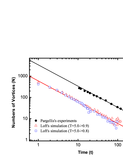
Figure 5: Number of defects versus time. Experimental and simulation results are shown. The results of simulation were the average of 20 quenches LD , for which $T^{*}=5.0$ initially and is suddenly reduced to $T^{*}=0.8$ ($\square$) and $T^{*}=0.9$ ($\triangle$). The experimental results, which are obtained by Pargellis et al Pa , were averaged over nine experimental runs ($\bullet$). Solid lines are the expected $N\propto t^{-1}$ scaling.

From the assumptions of dynamical scaling law, it has been predicted that the asymptotic growth law of the characteristic length is given by $\xi(t)\propto(t/lnt)^{1/2}$ Br02 ; however, scaling violations were reported. In a recent work, it was shown that the specific case of the 2D XY model is given as $\xi(t)\propto(t/lnt)^{1/2}$ if free vortices are present, while $\xi(t)\propto t^{1/2}$ if there are no free vortices present in the initial state Brprl . Since the topological current is identically conserved, there are no free vortices during the growth or annihilation process.

In the neighborhood of the bifurcation point, we denote scale length $\nabla x=l$. From Eqs. (51)-(53), we can then obtain the growth or annihilation velocity of the vortices, which is given as

$$v\propto const.$$ (60)

The approximation asymptotic relation of is then

$$\xi(t)\propto(t-t^{*}).$$ (61)

It can be seen that this is the reason why the relevant length of the vortices scales with time as $t^{-1/2}$ for small values of $t$ and then deviates towards a linear dependence in nematic liquid-crystal experimental observations Pa2 .

From Eq. (54), one can obtain

$$\xi(t)=const,\quad v=0.$$ (62)

It can be seen that that vortices are relatively at rest when $\xi(t)=const$.

During the growth or annihilation of vortices, the dynamical scaling law of the relevant length in the 2D XY model is given as $\xi(t)\propto(t-t^{*})^{1/2}$. This indicates that the vortices in the 2D XY model are the source of the scaling violations. During the crossing, splitting and merging of vortices, the dynamical scaling law of relevant length in the 2D XY model is given as $\xi(t)\propto(t-t^{*})$. However, if vortices are at rest during merging or splitting, the dynamical scaling law of relevant length is $\xi(t)=const$. Moreover, it is worth noting that the dynamical scaling law of vortices depends only on topological properties of the order parameter field.

V Conclusions

In summary, we have studied the inner structure and evolution of vortices in the 2D XY model by making using of the $\phi$-mapping topological current theory. A scalar field, $\psi$, is introduced through the topological current theory. By solving the scalar field, the interaction energy of vortices in the 2D XY model is revisited.

By using the $\phi$-mapping current theory, the densities of vortices in terms of the order parameter field in the 2D XY model are obtained directly from the definition of the topological charges of the vortices. The inner topological structure of the charge of the vortices, which is characterized by the Hopf index and the Brouwer degree, was obtained. By using the 2D topological current theorem, the Hamiltonian of the interaction vortices in the 2D XY model was revisited. This result is identical to the Hamiltonian of a 2D Coulomb gas with point charges of charge $W_{i}=\beta_{i}\eta_{i}$.

Furthermore, we have studied the evolution of vortices in the 2D XY model and concluded that there are crucial cases of branch processes in the evolution of vortices when $J^{0}(\phi/x)=0$ and $\phi=0$, i.e., $\eta_{l}$ is indefinite. It is important to note that according to the Landau-Ginzburg approach, there is instability in the 2D XY model at the zero point of the order parameter fields in the low temperature phase. This indicates that vortices are unstable in the low temperature phase. In the high temperature phase, the zero point of the order parameter field is stable. Due to the branch condition, the vortices generate or annihilate at the limit points and encounter, split, or merge at the bifurcation points of the order parameter field. This result also indicates that the velocity of the vortices is infinite when they are being annihilated or generated, which is obtained only from the topological properties of the order parameter field in the 2D XY model. The scaling law of relevant length, which is given as $R(t)\propto(t-t^{*})^{1/2}$, can be obtained in the neighborhood of the bifurcation point during the growth or annihilation of vortices. During the crossing, splitting and merging of vortices, the dynamical scaling law of relevant length is $\xi(t)\propto(t-t^{*})$. However, if vortices are at rest during merging or splitting, the dynamical scaling law of relevant length is $\xi=const$. The dynamical scaling law of vortices only depends on topological properties of the order parameter field.

Appendix A Topological Current theory

We study a two-component vector order parameter, $\vec{\phi}=(\phi^{1},\phi^{2})$, over the base manifold, M (in this paper $M=R^{2}\bigotimes R$):

$$\Psi=\phi^{1}+i\phi^{2},\quad\phi^{a}=\phi^{a}(x,y,t),\quad a=1,2.$$ (63)

Quantized defects are topological objects associated with topological properties of the order parameter $\Psi$. It is worth noting that the phase of the order parameter is undefined at the vortex core. In other words, vortices correspond to singularities of the order-parameter field. Let us define the unit vector field, $\vec{n}$, as:

$$n^{a}=\frac{\phi^{a}}{||\phi||},\quad||\phi||=\sqrt{\phi^{a}\phi^{a}},\quad a=1,2.$$ (64)

where, $n^{a}n^{a}=1$. From the unit vector, $\vec{n}(x)$, we can construct a topological current of the order parameter field in the 2D XY model, which carries the topological information of $\vec{\phi}(x)$:

$$j^{k}=\frac{1}{2\pi}\epsilon^{ijk}\epsilon_{ab}\partial_{i}n^{a}\partial_{j}n^{b},\quad i,j,k=0,1,2.$$ (65)

It can be seen that this current does not vanish only at the zero point of $\vec{\phi}(x)$, or the singularities of the unit field $\vec{n}(x)$. Obviously, the current given by Eq.(65) is identically conserved:

$$\partial_{k}j^{k}=0.$$ (66)

Suppose there is a vortex located at $z_{i}$. The topological charge of the defect is defined by the Gauss map, $n:\partial\sum_{i}\rightarrow S^{1}$:

$$W(\phi,z_{i})=\frac{1}{2\pi}\oint_{\partial\sum_{i}}\epsilon_{ab}n^{a}dn^{b}.$$ (67)

Using Stokes’ theorem in the exterior differential form, one can deduce that:

$$W(\phi,z_{i})=\frac{1}{2\pi}\oint_{\sum_{i}}\epsilon_{ab}\epsilon^{ij}\partial_{i}n^{a}\partial_{j}n^{b}d^{2}x.$$ (68)

Appendix B Two-dimensional topological current Theorem

By using the $\phi$-mapping method, we can prove that the topological current given by Eq. (65) is a $\delta$-like current:

$$j^{k}=\delta(\vec{\phi})J^{k}\left(\frac{\phi}{x}\right).$$ (69)

From the above formula, it can be seen that the topological current does not vanish only at the zero points of the vector field $\vec{\phi}(x)$.

Substituting Eq. (64) into Eq. (65) and considering that:

$$\partial_{k}n^{a}=\frac{\partial_{k}\phi^{a}}{||\phi||}-\phi^{a}\partial_{k}\left(\frac{1}{||\phi||}\right).$$ (70)

we have

$$j^{k}=\frac{1}{2\pi}\epsilon^{ijk}\epsilon_{ab}\partial_{i}\phi^{a}\partial_{j}^{b}\frac{\partial}{\partial\phi^{a}}\frac{\partial}{\partial\phi^{b}}(\ln(||\phi||)),$$ (71)

If we define the Jacobian as:

$$\epsilon^{ab}J^{k}\left(\frac{\phi}{x}\right)=\epsilon^{ijk}\partial^{j}\phi^{a}\partial^{k}\phi^{b},$$ (72)

and, by virtue of the Laplacian relation in $\phi$ space GS

$$\triangle_{\phi}\left(\ln(||\phi||)\right)=2\pi\delta^{2}(\vec{\phi}),$$ (73)

where

$$\triangle_{\phi}=\frac{\partial}{\partial\phi^{a}}\frac{\partial}{\partial\phi^{a}}$$

is the two-dimensional Laplacian operator in $\phi$ space, we obtain a $\delta$-function like current. This current is given by:

$$j^{k}=\delta(\vec{\phi})J^{k}\left(\frac{\phi}{x}\right).$$ (74)

From the above formula, one can see that the topological current does not vanish only at the zero points of the vector field $\vec{\phi}(x)$. Therefore, it is essential to investigate the solutions of $\vec{\phi}(x)=0$.

- (1) N. D. Mermin, Phys. Rev 176, 250 (1968); N. D. Mermin and H. Wagner, Phys. Rev. Lett. 22, 1133 (1966); V. L. Berezinskii, Sov. Phys.-JETP, 32, 493 (1970); H. E. Stanley and T. A. Kaplan, Phys. Rev. Lett 17, 913 (1966); J. M. Kosterlitz and D. J. Thouless, J. Phys. C 6, 1181 (1973).
- (2) K. J. Strandburg, Rev. Mod. Phys. 60, 161 (1988).
- (3) D. R. Nelson, Defects and Geometry in Condensed Matter Physics, (Cambridge University Press, Cambridge, 2002).
- (4) P. M. Chaikin and T. C. Lubensky, Principles of condensed matter physics, (Cambridge University Press, Cambridge, 1995).
- (5) B. I. Halperin, Physics of Defects, edited by R. Balian et al. (North-Holland, Amsterdam, 1981).
- (6) F. Liu and G. F. Mazenko, Phys. Rev. B 46, 5963 (1992).
- (7) Y. S. Duan, H. Zhang, and L. B. Fu, Phys. Rev. E 59, 528 (1999).
- (8) H. Kleinert, Gauge Theory in Condensed Matter, (World Scientific, Singapore, 1989).
- (9) J. Zaanen, Z. Nussinov and S. I. Mukhin, Ann. Phys(New York) 310, 181(2004); V. Cvetkovic, Z. Nussinov, S. Mukhin, and J. Zaanen, Europhys. Lett 81, 27001 (2007).
- (10) Y. S. Duan and S. L. Zhang, Int. J. Eng. Sci. 29, 1593 (1991); G. H. Yang and Y. S. Duan, Int. J. Theor. Phys. 37, 2371 (1998); Y. S. Duan and H. Zhang, Phys. Rev. E 60, 2568 (1999).
- (11) Y. S. Duan and H. Zhang, Eur. Phys. J. D 5, 47 (1999).
- (12) Y. S. Duan, H. Zhang, and S. Li, Phys. Rev. B 58, 125 (1998).
- (13) A. J. Bray, Adv. Phys. 43, 357 (1994).
- (14) B. Zheng, Int. J. Mod. Phys. B 12, 1419 (1998).
- (15) A. J. Bary and A. D. Rutenberg, Phys. Rev. E 49, R27 (1994).
- (16) H. K. Janssen, B. Schaub, and B. Schmittmann, Z. Phys.B 73, 539 (1989).
- (17) A. J. Bray, A. J. Briant, and D. K. Jervis. Phys. Rev. Lett 84, 1503 (2000).
- (18) R. Loft and T. A. DeGrand, Phys. Rev. B 35, 8528 (1987).
- (19) A. N. Pargellis, S. Green, and B. Yurke, Phys. Rev. E 49, 4250 (1994).
- (20) A. N. Pargellis, P. Finn, J. W. Goodby, P. Panizza, B. Yurke and P. E. Cladis, Phys. Rev. A 46, 7765 (1992).
- (21) M. Kubicek and M. Marek, Computational Methods in Bifurcation Theory and Dissipative Structures, (Springer, New York, 1983).
- (22) A. J. Bray, Phys. Rev. E 55, 5297 (1997).
- (23) T. Xu, Phys. Rev. E 72, 036303 (2005).
- (24) I. M. Gel’fand and G. E. Shilov, Generalized Function, (Academic, New York, 1964) Vol. 1.