Nonlinear aspects of astrobiological research

Abstract

Several aspects of mathematical astrobiology are discussed. It is argued that around the time of the origin of life the handedness of biomolecules must have established itself through an instability. Possible pathways of producing a certain handedness include mechanisms involving either autocatalysis or, alternatively, epimerization as governing effects. Concepts for establishing hereditary information are discussed in terms of the theory of hypercycles. Instabilities toward parasites and possible remedies by invoking spatial extent are reviewed. Finally, some effects of early life are discussed that contributed to modifying and regulating atmosphere and climate of the Earth, and that could have contributed to the highly oxidized state of its crust.

Glossary

Chiral, achiral and racemic

A molecule is chiral if its three-dimensional structure is different from its mirror image. Such molecules tend to be optically active and turn the polarization plane of linearly polarized light in the right or left handed sense. Correspondingly, they are referred to as D- and L-forms, which stands for dextrorotatory and levorotatory molecules. An achiral molecule is mirror symmetric and does not have this property. A substance is racemic if it consists of equally many left and right handed molecules. A polymer is said to be isotactic if all its elements have the same chirality.

Enantiomers and enantiomeric excess

Enantiomers denote a pair of chiral molecules that have opposite handedness, but are otherwise identical. Enantiomeric excess, usually abbreviated as e.e., is a normalized measure of the degree by which one handedness dominates over the other one. It is defined as the ratio of the difference to the sum of the two concentrations, so e.e. is between $-1$ and $+1$.

Epimerization and racemization

Epimerization is the spontaneous change of handedness of one sub-unit in a polymer. Racemization indicates the loss of a preferred handedness in a substance.

Catalysis and auto-catalysis

Catalysts are agents that lower the reaction barrier. A molecule reacts with the catalyst, but at the end of the reaction the catalyst emerges unchanged. This is called catalysis. In auto-catalysis the catalyst is a target molecule itself, so this process leads to exponential amplification of the concentration of this molecule by using some substrate. Biological catalysts are referred to as enzymes.

Nucleotides and nucleic acids

Nucleotides are the monomers of nucleic acids, e.g. of RNA (ribonucleic acid) or DNA (deoxyribonucleic acid). They contain one of four nucleobases (often just called bases) that can pair in a specific way. Nucleotides can form polymers and their sequence carries genetic information. One speaks about a polycondensation reaction instead of polymerization because one water molecule is removed in this step. Other nucleotides of interest include peptide nucleic acid or PNA. Here the backbone is made of peptides instead of sugar phosphate.

Peptides and amino acids

Amino acids are molecules of the general form NH₃–CHR–COOH, where R stands for the rest, which makes the difference between different amino acids. For glycine, the simplest amino acid, we have R=H, so two of the bonds on the central C atom are the same and the molecule is therefore chiral. For alanine, R=CH₃, so all four bonds on the central C atom are different, so this molecule is chiral. A peptide is a polymer generated through a polycondensation reaction of amino acids. Peptides are also referred to as proteins.

Solar constant and albedo

The solar constant is the total flux of energy from the Sun above the Earth atmosphere. Its current value is $S=1.37\,{\rm kW}\,{\rm m}^{-2}$, but it has been about 30% lower when the solar system was young ($10^{8}\,{\rm yr}$ old, say), so $S$ is not a constant. The albedo $A$ is the fraction that is reflected from the surface of the Earth, e.g. by clouds and snow and, to a lesser extend, by land masses and oceans.

Photosynthesis and carbon fixation

Photosynthesis uses light to reduce CO₂ and to produce oxygen either as free molecular oxygen or in some other chemical form. This process removes CO₂ from the atmosphere and produces biomass, which is written in simplistic form as $(\mbox{CH}_{2}\mbox{O})_{n}$. This process is referred to as carbon fixation.

Life

A preliminary definition of life involves replication and death, coupled to a metabolism that utilizes any sort of available energy. Life is characterized further by natural selection to adapt to environmental changes and to utilize available niches. A proper definition of life is difficult given that all life on Earth can be traced back to a single common ancestor. Any definition of life may need to be adjusted if extraterrestrial or artificial life are discovered.

Definition of the subject

Astrobiology is concerned with questions regarding possible origins of life on Earth and elsewhere in the Universe. Although there is presently no detection of extraterrestrial life, it is generally assumed that life could be wide-spread provided certain conditions of habitability are met. A common implicit hypothesis in astrobiology is that life can emerge spontaneously once certain environmental conditions are met. This implies that there may well have been multiple geneses, separated only by global extinction events such as major impacts by other celestial bodies [1].

Four important discoveries can be named that have provided impetus to the field of astrobiology.

1. More than 300 extrasolar planets have been discovered since 1995, providing explicit targets for detecting life outside the solar system.

2. Recent Mars missions have provided evidence for liquid water on the surface of Mars in past and possibly even present times. This has fostered the search for techniques to detect microbial life on Mars.

3. On Earth the carbon in very old sedimentary rocks dating back 3.8 Gyr ago show a consistently lower ¹³C to ¹²C abundance ratio. This is normally indicative of life. This lends support to the notion that life may have been present as soon as the Earth surface became hospitable.

4. The discovery of extremophiles on Earth has considerably extended the definition of habitability to include extreme temperatures, pressures and pH values, high salinity as well as high radiation levels. This has raised hopes of finding life even in our solar system.

Astrobiology thus comprises several scientific disciplines: astronomy, geology, chemistry, and biology. Therefore, much of the original literature tends to appear in journals in the respective fields. We should also mention that there are technological attempts in producing artificial life [2]. While this approach is not aimed at reproducing the origin of life on Earth, it may still be useful for feeding our imagination in understanding the transition from nonliving to living matter.

1 Introduction

Since the early days of nonlinear dynamics and non-equilibrium thermodynamics it has been clear that one of the ultimate applications of this theory might be to facilitate an understanding of the transition from non-living to living matter. The main reason is obviously that living systems are very far from equilibrium—as indicated by the high degree of order and hence the low entropy of living systems relative to their exterior.

Already in 1952 Turing [3] proposed the idea that chemical reaction-diffusion systems might provide a tool for studying biochemical pattern formation which have increased our understanding of the laws of nature far from equilibrium, where life occurs. This idea was followed up in the late 1960s by Prigogine [4, 5] who suggested that dissipative structures have great importance in establishing a physical description of living matter. A general theory of autocatalytic molecular evolution was developed in 1971 by Eigen [6] who argued that in a single micro-environment only a single handedness can result from a single event. In particular the famous chicken and egg problem that occurs in biology at different levels was identified as a Hopf bifurcation. A Hopf bifurcation describes the spontaneous emergence of an oscillating solution once some stability threshold has been crossed. The mathematics of this is familiar to any physicist, but it requires that the equations describing the relevant physics are known. In biology it is not even clear that the various phenomena can be described by equations. A first detailed attempt in this direction was indeed that of Eigen. However, the equations governing the emergence of life are only phenomenological ones. Nevertheless, these approaches are invaluable in that they help giving the origin of life question a mathematical basis.

One of the earliest anticipated forms of life that is still similar to present life is the RNA world [7], whereby simple RNA molecules with functional behavior self-reproduces using genetic information encoded either in the same or in other participating RNA molecules. Obviously, there are tremendous difficulties given that RNA is too complicated a molecule to be synthesized abiologically. A significantly simpler molecule is peptide nucleic acid or PNA [8], where the backbone consists of peptide instead of sugar phosphate. Nevertheless, the difficulty of producing RNA remains.

There is no firm idea where on Earth such molecular replication may have taken place. Frequently discussed scenarios include hydrothermal vent systems [9], but also beach scenarios are discussed that are subject to tides leading to cyclic changes in concentration [10] as well as to repeated wetting and drying [11].

An early experiment that contributed significantly to the research into origins of life was the Urey–Miller experiment [12] that demonstrated the spontaneous production of amino acids in a reducing atmosphere consisting of H₂O vapor, CH₄, NH₃, and H₂ with an energy supply in the form of sparks. More recent experiments also allow for the presence of CO₂, which now seems unavoidable on the early Earth given that it is continuously replenished through outgassing by volcanoes.

In the following we review some aspects where there has been considerable cross-fertilization between astrobiology and nonlinear dynamics. We begin by discussing a phenomenon that is believed to have taken place around the time of the origin of life, namely the establishment of a definitive handedness of biomolecules that is inherent to DNA and RNA (D-form) and to amino acids (L-form). Next we discuss constraints on the evolution of hereditary information, and finally review some models that characterize the alteration of the terrestrial environment by early life. In addition to any of these physical effects there are random fluctuations leading inevitably to local imbalances between the concentrations of molecules of D- and L-form. In the following we discuss mechanisms that can lead to an exponential amplification of the enantiomeric excess. For a recent review of these ideas see Ref. [13].

2 Homochirality

Theories of a chemical origin of life involve polymerization of nucleotides that carry and utilize genetic information. Ribonucleotides possess chirality, i.e. they are different from their mirror image. All known life forms use ribonucleotides of the so-called D-form (right-handed), as opposed to the L-form (left-handed). These two molecules are referred to as opposite enantiomers. In most cases these different enantiomers are optically active, i.e. they turn the polarization plane of linearly polarized light in a right-handed or left-handed sense.

Any non-enzymatic synthesis of ribonucleotides would have produced a mixture of equally many right- and left-handed building blocks. Technically this is referred to as a racemic mixture of these molecules. However, experimentally it is known that in a racemic mixture of mononucleotides the polymerization is quickly terminated after the first or second polymerization step [14]. This is generally referred to as enantiomeric cross-inhibition, which was long thought to be a serious obstacle to a chemical origin of life. It was therefore thought to be necessary that life evolved only in a homochiral environment. Moreover, it would then be necessary that the degree of enantiomeric purity must have been very high. This is important because it rules out a number of physical mechanisms based on the enantioselective effects of circularly polarized radiation, magnetic fields, and the parity-breaking property of the electroweak force.

2.1 The Frank-mechanism

A general mechanism for producing complete homochirality was proposed in 1953 by Frank [15] based on the assumed effects of auto-catalysis and what he called mutual antagonism. In fact, the enantiomeric cross-inhibition mentioned above can be thought of as a possible example of mutual antagonism. The model of Frank is characterized by the following set of three reactions:

$$D+S\stackrel{{\scriptstyle k_{C}}}{{\longrightarrow}}D+D,$$ (1)

$$L+S\stackrel{{\scriptstyle k_{C}}}{{\longrightarrow}}L+L,$$ (2)

$$D+L\stackrel{{\scriptstyle k_{I}}}{{\longrightarrow}}DL,$$ (3)

where $D$ and $L$ denote monomers of the two enantiomers, $S$ is a substrate from which monomers could be formed via auto-catalysis, and $DL$ are inactive dimers that are lost from the system. (At this level of simplification no distinction between $DL$ and $LD$ is made. This simplification will later be relaxed.) The parameters $k_{C}$ and $k_{I}$ characterize the reaction speeds. These reactions translate to the following set of equations for the concentrations of $D$, $L$, $S$, and $DL$,

$${{\rm d}{}\over{\rm d}{}t}[D] = +k_{C}[S][D]-k_{I}[D][L],$$ (4)

$${{\rm d}{}\over{\rm d}{}t}[L] = +k_{C}[S][L]-k_{I}[D][L],$$ (5)

$${{\rm d}{}\over{\rm d}{}t}[S] = -k_{C}[S]\Big{(}[D]+[L]\Big{)},$$ (6)

$${{\rm d}{}\over{\rm d}{}t}[DL] = +2k_{I}[D][L].$$ (7)

These equations imply that the total mass of all building blocks (including the substrate), is constant, i.e. $[D]+[L]+[S]+[DL]=\mbox{const}\equiv M$.

Figure 1: Solution of Eqs. (4)–(6) for $k_{I}=k_{C}$. Both $D$ and $L$ grow exponentially until $[D]+[L]$ becomes comparable to the constantly declining substrate concentration $[S]$. At the same time the production of $DL$ removes an equal amount of $D$ and $L$, but this effect affects mostly those enantiomers that are already in the minority. In this calculation an initial asymmetry (here 10%) of $[D]-[L]$ grows until saturation. At the end, $[D]$ has reached 100% enantiomeric excess, but this happened at the expense of producing a large number of inactive heterochiral dimers $DL$.

This system of equations describes the continued autocatalytic production of $DL$, $D$ and $L$ until the substrate $S$ is exhausted, i.e. $[S]=0$. However, as long as $[S]$ is still finite, the asymmetry, ${\cal A}=[D]-[L]$, grows quasi-exponentially, proportional to $\exp(\int[S]\,{\rm d}{}t)$. A numerical example of this is shown in Fig. 1.

In the numerical example above we started with very small initial concentrations. Another possibility is to start with a perturbed racemic solution. The racemic solution is given by $[D]=[L]=\lambda/k_{I}$, where $\lambda=k_{C}[S]$ is the instantaneous growth rate due to autocatalysis. Under the assumption that $\lambda$ can be treated as a constant (i.e. when the system is still nearly racemic), a linear stability analysis shows that the enantiomeric excess,

$$\mbox{e.e.}={[D]-[L]\over[D]+[L]}$$ (8)

grows exponentially. This means that the racemic solution is unstable and that the mechanism for achieving homochirality is based on a linear instability.

2.2 Continued polymerization

There is a priori no good reason to permit the production of heterochiral dimers $DL$, but not of homochiral dimers $DD$ and $LL$, i.e.

$$D+D\stackrel{{\scriptstyle k_{S}}}{{\longrightarrow}}DD,$$ (9)

$$L+L\stackrel{{\scriptstyle k_{S}}}{{\longrightarrow}}LL.$$ (10)

The importance of such reactions was stressed in a review by Blackmond [16], who also introduced an additional modification that consists in the assumption that not the monomers, but the homochiral dimers $DD$ and $LL$ catalyze the production of monomers, i.e. reactions (1) and (2) are replaced by

$$DD+S\stackrel{{\scriptstyle k_{C}}}{{\longrightarrow}}DD+D,$$ (11)

$$LL+S\stackrel{{\scriptstyle k_{C}}}{{\longrightarrow}}LL+L.$$ (12)

This model is similar to the original Frank model provided there is a way of getting rid of those homochiral dimers that are in the minority. This requires enantiomeric cross-inhibition for dimers to form heterochiral trimers, i.e. we need the additional reactions

$$DD+L\stackrel{{\scriptstyle k_{I}}}{{\longrightarrow}}DDL,$$ (13)

$$LL+D\stackrel{{\scriptstyle k_{I}}}{{\longrightarrow}}LLD.$$ (14)

A solution to the corresponding reaction equations is given in Fig. 2. Reaction calorimetry is able to give support to the assumption that dimers and not monomers are the relevant catalysts [16]. This seems to apply in particular to the first autocatalytic reaction ever found that enhances enantiomeric excess [17]. In this reaction (sometimes referred to as the Soai reaction) the substrate is pyridine-3-carbaldehyde and the chiral molecule of either D- or L-form is 3-pyridyl alkanol which thus acts as an asymmetric autocatalyst to produce more of itself. In this reaction, however, dialkylzinc acts as an additional achiral catalysts. While the Soai reaction is important as a first explicit example of an autocatalytic reaction that enhances the enantiomeric excess, it is not normally regarded as directly important for astrobiology.

Figure 2: Solution of Eqs. (4)–(6) supplemented by the kinetic equations corresponding to the reactions Eqs. (9)–(14), for $k_{S}=k_{I}=k_{C}$. Again, an initial 10% asymmetry of $[D]-[L]$ grows until $[D]+[L]$ becomes comparable to the constantly declining substrate concentration $[S]$. The monomers polymerize into dimers $DD$ and $LL$. Toward the end, $[DD]$ reaches a 100% enantiomeric excess

The polymerization model has been developed by Sandars [18], who included arbitrarily many polymerization steps of the form

$$D_{n}+D\stackrel{{\scriptstyle k_{S}}}{{\longrightarrow}}D_{n+1},$$ (15)

$$L_{n}+L\stackrel{{\scriptstyle k_{S}}}{{\longrightarrow}}L_{n+1},$$ (16)

$$D_{n}+L\stackrel{{\scriptstyle k_{S}}}{{\longrightarrow}}D_{n}L,$$ (17)

$$L_{n}+D\stackrel{{\scriptstyle k_{S}}}{{\longrightarrow}}L_{n}D.$$ (18)

The basic outcome of this and similar models is always the same as in the original Frank model, except that the polymerization model is also capable of displaying interesting wave-like dynamics in time-dependent histograms of different polymers [19].

2.3 Spatially extended models

In reality there are limits as to how much a system can be considered fully mixed. In general, $[D]$ and $[L]$ should be functions of time and space, i.e. $[D]=[D](t,\mbox{\boldmath$x$}{})$ and $[L]=[L](t,\mbox{\boldmath$x$}{})$. Assuming that there is only molecular diffusion, the relevant reaction equations are to be supplemented by additional diffusion terms,

$${{\rm d}{}\over{\rm d}{}t}[D_{n}]=R_{n}^{(D)}+\kappa\nabla^{2}[D_{n}],$$ (19)

$${{\rm d}{}\over{\rm d}{}t}[L_{n}]=R_{n}^{(L)}+\kappa\nabla^{2}[L_{n}],$$ (20)

where $R_{n}^{(D)}$ and $R_{n}^{(L)}L$ are the right hand sides of the reaction equations.

If there were only one type of handedness, the resulting equation would be reminiscent of the Fisher equation [20],

$${{\rm d}{}f\over{\rm d}{}t}=\lambda(1-f)f+\kappa\nabla^{2}f,$$ (21)

which admits propagating front solutions with front speed $v_{\rm front}=2\sqrt{\kappa\lambda}$. Here, $f$ could represent the local concentration of some disease in models of the spread of epidemics, for example.

In the present case there are two fields, one of each handedness. It is instructive to refer to these fields as populations which is suggestive of their ability to replicate, migrate. become extinct, and to compete against a population of opposite handedness. Each population is able to expand into unpopulated space at a speed given approximately by $v_{\rm front}$, but once two opposing handednesses come into contact, there is an impasse and the propagation comes to a halt. A snapshot of a one-dimensional model illustrating the polymer length as a function of position is shown in Fig. 3 for populations of opposite handedness that have come into contact.

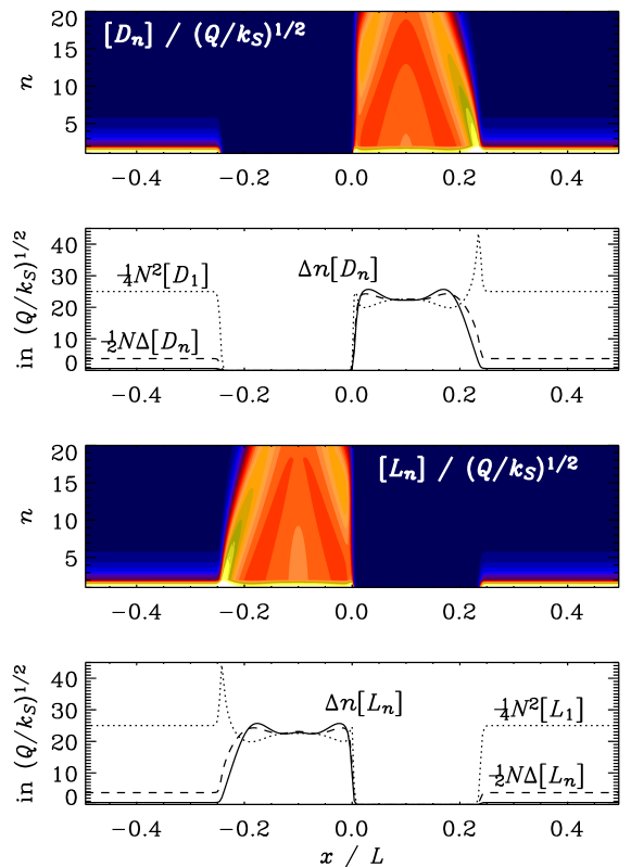
Figure 3: Color/gray scale plots of $[D_{n}]$ and $[L_{n}]$ for $t/\tau_{\rm diff}=0.8$ as a function of $x$ and $n$, and the corresponding dependencies of $\sum_{n=1}^{N}n[D_{n}]$ and $\sum_{n=1}^{N}n[L_{n}]$ (solid line), compared with ${\textstyle{1\over 2}}N\sum_{n=1}^{N}[D_{n}]$ and ${\textstyle{1\over 2}}N\sum_{n=1}^{N}[L_{n}]$ (dashed line), and ${\textstyle{1\over 4}}N^{2}[D_{1}]$ and ${\textstyle{1\over 4}}N^{2}[L_{1}]$ (dotted line), all in units of $(Q/k_{S})^{1/2}$. The normalized diffusivity is $\kappa/(L^{2}\lambda_{0})=10^{-2}$ and $N=20$. Adapted from Ref. [21].

The overall dynamics of symmetry breaking is well characterized by a low order truncation, where the model is truncated at $n=2$ and the evolution of the $n=1$ modes is assumed to be enslaved by the evolution of the $n=2$ modes [19]. An example of such a solution is shown in Fig. 4, which shows the evolution in a space-time diagram, where two populations of opposite handedness expand into unpopulated space until two opposite populations come into contact.

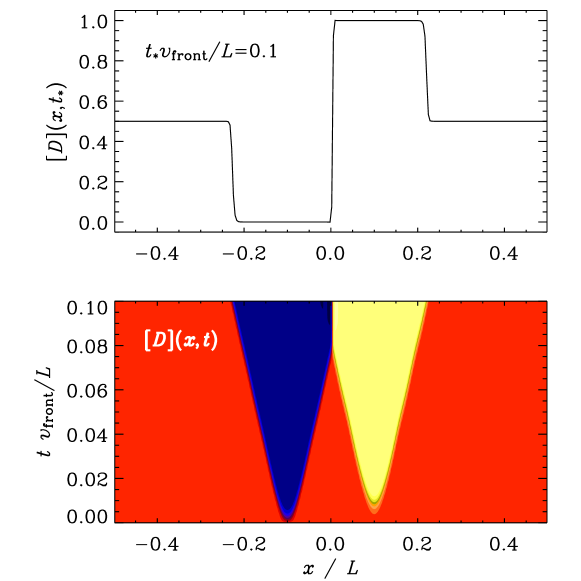
Figure 4: Profile of $[D](x,t_{*})$ and space-time diagram of $[D](x,t)$ for the one-dimensional problem without advection and an initial perturbation corresponding to a weak (amplitude 0.01) right-handed excess at $x/L=0.1$ (marked in white or yellow) and a somewhat stronger (amplitude 0.3) left-handed excess at $x/L=-0.1$ (marked in dark or blue). Note the propagation of fronts with constant speed if the exterior is racemic (i.e. $[D]=[L]=1/2$, shown in medium shades or red) and a nonpropagating front when the chirality is opposite on the two sides of the front. The normalized diffusivity is $\kappa/(L^{2}\lambda_{0})=10^{-2}$, i.e. the same as in Fig. 3. Adapted from Ref. [21].

In two and three dimensions a front between two opposing enantiomers is in general curved, in which case it can propagate diffusively in the direction of curvature. This is caused by the fact that the inner front between two populations is slightly shorter than the outer one. (Only the immediate proximity of a front matters; what lies behind it is irrelevant if it is of the same handedness.) Indeed, on a two-dimensional surface the inner front is by $2\pi d$ shorter than the outer one—independent of radius. Here, $d$ is the front thickness, which is of the order of $d\approx(\kappa/\lambda)^{1/2}$.

It turns out that in two dimensions the rate of change of the integrated asymmetry, ${\cal A}=\int([D]-[L])\,{\rm d}{}^{2}x$, depends only on the number of topologically distinct rings or islands. Once an island is wiped out, the rate of change of ${\cal A}$ changes abruptly and stays then constant until the next island gets wiped out. So the enantiomeric excess,

$$\mbox{e.e.}={\int([D]-[L])\,{\rm d}{}^{2}x\over\int([D]+[L])\,{\rm d}{}^{2}x},$$ (22)

increases with time in a piecewise linear fashion.

Even if at each point homochirality could be reached rapidly (time scale $\lambda^{-1}$), global homochirality requires that one population wipes out the other one completely. Diffusion is usually too slow to lead to any significant mixing and hence to global homochirality. However, there could be circumstances where such mixing is sped up by something like “turbulent” transport. In the case of the Earth the slowest relevant transport is in the Earth mantle, part of which is now associated with what is called the deep biosphere. Assuming that multiple geneses of life is possible, this would raise the question whether a simultaneous co-existence of different handednesses on different parts of the early Earth would have been possible. It is however unclear whether this possibility could have left any traces that would still be detectable today.

Another approach to solving the problem of spatially extended chemistry is by means of cellular automata. In this approach points on a mesh can take different states corresponding to molecules of right or left handedness, achiral substrate molecules, or even empty states. An example of such a calculation by Shibata et al. [22] is shown in Fig. 5. Again, there are patches of populations of opposite handedness that grow and wipe each other out such that in the end only one handedness survives.

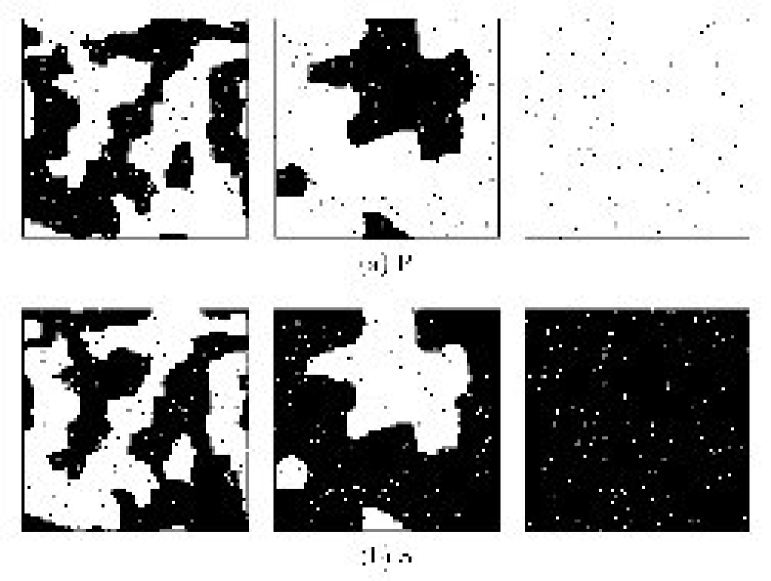
Figure 5: The evolution of molecules of D- and L-forms is shown in the upper and lower panels, respectively. Note the tendency toward complete homochiralization by gradually filling up isolated islands with the chirality of the surrounding molecules. The dimensionless times are 50, 250, and 1750 from left to right. Courtesy of Shibata et al. [22].

2.4 Epimerization

An interesting alternative to the Frank-type mechanism is a set of reactions based primarily on a phenomenon called epimerization, i.e. the spontaneous change of handedness in one part of the polymer. This mechanism is important in the chemistry of amino acids. Plasson et al. [23] identified four reactions: activation, polymerization, epimerization, and depolymerization as necessary ingredients that can, under certain conditions, lead to an instability of the racemic state with a bifurcation toward full homochirality. They called this the APED model, whose reactions can be summarized as follows:
A: activation:

$$L\stackrel{{\scriptstyle a}}{{\longrightarrow}}L^{*},\quad D\stackrel{{\scriptstyle a}}{{\longrightarrow}}D^{*},$$ (23)

P: polymerization:

$$L^{*}+L\stackrel{{\scriptstyle p}}{{\longrightarrow}}LL,\quad D^{*}+D\stackrel{{\scriptstyle p}}{{\longrightarrow}}DD,$$ (24)

$$L^{*}+D\stackrel{{\scriptstyle\alpha p}}{{\longrightarrow}}LD,\quad D^{*}+L\stackrel{{\scriptstyle\alpha p}}{{\longrightarrow}}DL,$$ (25)

E: epimerization:

$$LD\stackrel{{\scriptstyle e}}{{\longrightarrow}}DD,\quad DL\stackrel{{\scriptstyle e}}{{\longrightarrow}}LL,$$ (26)

D: depolymerization:

$$LL\stackrel{{\scriptstyle h}}{{\longrightarrow}}L+L,\quad DD\stackrel{{\scriptstyle h}}{{\longrightarrow}}D+D.$$ (27)

This minimal subset of reactions is shown in Fig. 6.

Figure 6: Representation of the minimal set of reactions necessary for allowing the spontaneous transition to homochirality. Adapted from Ref. [24].

Compared with the Frank model, a major advantage of the present model is that no hypothetical auto-catalysis is required. Indeed, all these reactions exist in principle, although it is as yet unclear what kind of manipulations on the environment are required to make all these reactions happen. Another advantage is that the system is closed, so no inflow or outflow of matter is required. The system is maintained away from equilibrium by energy input though the activation of amino acids.

Given that there is neither auto-catalysis nor enantiomeric cross-inhibition, one wonders whether the APED model still shares some similarities with Frank’s original model. Some degree of similarity is immediately seen by writing the APED reactions in sequential form in one line, i.e.,

$$D^{*}+L\stackrel{{\scriptstyle\alpha p}}{{\longrightarrow}}DL\stackrel{{\scriptstyle e}}{{\longrightarrow}}LL\stackrel{{\scriptstyle h}}{{\longrightarrow}}L+L,$$ (28)

$$L^{*}+D\stackrel{{\scriptstyle\alpha p}}{{\longrightarrow}}LD\stackrel{{\scriptstyle e}}{{\longrightarrow}}DD\stackrel{{\scriptstyle h}}{{\longrightarrow}}D+D.$$ (29)

This shows that, as long as the reaction rates for epimerization and depolymerization are not limiting factors, we have essentially the reactions

$$D^{*}\stackrel{{\scriptstyle\alpha pL}}{{\longrightarrow}}L\quad\mbox{and}\quad L^{*}\stackrel{{\scriptstyle\alpha pD}}{{\longrightarrow}}D.$$ (30)

This way of writing these reactions emphasizes the roles of $L$ and $D$ in catalyzing the conversion of $D^{*}$ into $L$ and $L^{*}$ into $D$, respectively. Just like the mechanism of mutual antagonism, these reactions disfavor a racemic state, but instead of producing unreactive waste, these reactions produce directly one of two possible homochiral states.

In addition, there are reactions of the form

$$L^{*}+L\stackrel{{\scriptstyle p}}{{\longrightarrow}}LL\stackrel{{\scriptstyle h}}{{\longrightarrow}}L+L,$$ (31)

$$D^{*}+D\stackrel{{\scriptstyle p}}{{\longrightarrow}}DD\stackrel{{\scriptstyle h}}{{\longrightarrow}}D+D.$$ (32)

These reactions simulate the autocatalytic conversion of $L^{*}$ into $L$ by $L$ and of $D^{*}$ into $D$ by $D$. Again, linear analysis establishes that the racemic state is unstable provided $\alpha$ is in the range $0<\alpha<1$; see Refs. [23, 24].

In conclusion we can say that the homochirality of life-bearing molecules might well have originated from the chemical reactions that lead to their formation. Thus, the hypothetical RNA world may have been born into an environment surrounded by homochiral peptides (as described in Section 2.4), or, alternatively, homochirality may have emerged as a consequence of enantiomeric cross-inhibition during the first stages of the RNA world (as discussed in Section 2.2).

In the next section we discuss some issues regarding possible strategies for establishing a primitive information-carrying system. This is also based on catalysis, but catalysis in the production of other molecules than itself.

3 Establishing hereditary information

We have so far ignored the fact that polymers can consist of different amino acid or nucleotide units, even though they would all have the same handedness. Therefore such molecules could in principle carry information. Once such polymers can replicate, the question arises how to prevent them from getting extinct due to errors in the copying process, and instead to compete against parasites. It is generally believed that early self-replicating systems had a substantial error rate associated with each replication event. A certain small error rate is obviously necessary for facilitating Darwinian evolution by natural selection, but it must be small enough to prevent extinction.

Figure 7: Number of survivors as a function of the number of generations in a numerical example with an error rate of $p=0.01$. This initial number of survivors is 1000. Note that for a genome length of $N=70$ and 71 the population dies out after 1800 and 400 generations, respectively. For $N=69$ and less the number of survivors increases exponentially. This is compatible with the survival criterion $N\mathrel{\mathchoice{\vbox{\offinterlineskip\halign{\hfil$\displaystyle#$\hfil\cr<\cr\sim\cr}}}{\vbox{\offinterlineskip\halign{\hfil$\textstyle#$\hfil\cr<\cr\sim\cr}}}{\vbox{\offinterlineskip\halign{\hfil$\scriptstyle#$\hfil\cr<\cr\sim\cr}}}{\vbox{\offinterlineskip\halign{\hfil$\scriptscriptstyle#$\hfil\cr<\cr\sim\cr}}}}(\ln 2)/0.01=69.3$, derived from Eq. (33).

Assuming that with each generation a species produces $\sigma$ offspring where the length of the genome is $N$ bits, and that the probability for a copying error at any position in the genome is $p$, the necessary condition for long-term survival is given by [6, 25]

$$pN<\ln\sigma.$$ (33)

The significance of this formula is illustrated in Fig. 7 with the help of a numerical example where the selective advantage (i.e. the multiplication factor) is chosen to be $\sigma=2$, the error rate is $p=0.01$, and four different values of $N$ between 68 and 71 are used. In this numerical experiment, $\sigma$ new offspring are produced, but with a probability $p$ an error is introduced at each of the $N$ positions. After this only the intact copies can produce further offspring, and so forth.

According to Eq. (33) the maximum genome length is, with the parameters of our example, $(\ln 2)/0.01=69.3$. This is compatible with Fig. 7 which shows that the dividing line between extinction and long-term survival is between $N=69$ and 70. For contemporary genomes $N$ is of the order of $10^{8}$, and $p$ is of the order of $10^{-8}$ [26], or below, depending on the efficiency of error-correcting mechanisms that are available in contemporary organisms.

The first replicating systems are likely to have rather high error rates, and no correction mechanism, making it virtually impossible to carry sufficient information for building more complex replicators. This difficulty can be removed by invoking the concept of hypercycles [27], whereby the full genetic information is carried collectively by several smaller systems (smaller $N$), each one small enough to obey Eq. (33). Mathematically, such a system can be described by the following set of reactions [28]:

$$I_{i}\stackrel{{\scriptstyle r_{i}}}{{\longrightarrow}}2I_{i},$$ (34)

$$I_{i}+I_{i-1}\stackrel{{\scriptstyle k_{i}}}{{\longrightarrow}}2I_{i}+I_{i-1}.$$ (35)

Assuming furthermore that resources are limited, the total number of molecules, $M=\sum_{i}[I_{i}]$, is taken to be constant, i.e. $I_{i}$ is assumed to be siphoned off from the system at a rate $\phi$ that is independent of $i$. Mathematically, such a system can be described by the following set of ordinary differential equations:

$${{\rm d}{}\over{\rm d}{}t}[I_{i}]=r_{i}[I_{i}]+k_{i}[I_{i}][I_{i-1}]-\phi[I_{i}],$$ (36)

where

$$\phi=\sum_{i}\Big{(}r_{i}[I_{i}]+k_{i}[I_{i}][I_{i-1}]\Big{)}\left/\sum_{i}[I_{i}]\right.$$ (37)

is the factor that keeps the total number of molecules constant. The kinetic coefficient $r_{i}$ models the residual effects of birth and death, while $k_{i}$ is the kinetic coefficient for the catalytic production of $I_{i}$, where $I_{i-1}$ acts as a catalyst. The evolution of number densities in a model of five hypercycles is shown in Fig. 8 for a case where all $k_{i}=k$ and $r_{i}=r$ are chosen to be the same for all values of $i$.

Figure 8: Evolution of the number densities of five hypercycles with equal parameters. Note that peaks of $I_{1}$ (solid line) are followed by peaks of $I_{2}$ (dotted line) and $I_{3}$ (dashed line), and so forth. Time is measured in units of $r^{-1}$ and concentrations are measured in units of $r/k$.

An interesting situation arises when the effects of parasites are included. Boerlijst & Hogeweg [28] considered an example where a parasite is coupled to $I_{2}$; see Eq. (9). The effect on the above model is shown in Fig. 10 where $k_{\rm para}=2k$ and $r_{\rm para}=r$ has been chosen. One sees that not much happens for a long time when the parasite is turned on. This is because the parasite has to grow to a level where it can affect the entire system. When this point is reached, all components of the system decay exponentially—including the parasite itself. Unfortunately, the system can never recover from this disaster, so the hypercycle theory seems to have a problem.

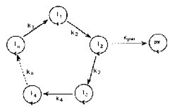
Figure 9: Sketch showing the coupling of several hypercycles together with a parasite coupled to species $I_{2}$. Courtesy of M.C. Boerlijst & P. Hogeweg [28].

Figure 10: Evolution of the number densities of five hypercycles with equal parameters and a parasite where $k_{\rm para}=2k_{i}$ and $r_{\rm para}=r$. Time is measured in units of $r^{-1}$ and concentrations are measured in units of $r/k$.

Again, spatial extent can significantly alter the situation. Using a cellular automata approach, Boerlijst & Hogeweg [28] showed that the danger of parasitic catastrophes can be eliminated by allowing the offspring to enter unpolluted areas faster than the growth of the parasite allows. Interestingly enough, this approach tends to produce spiraling interfaces between different species; see Fig. 11.

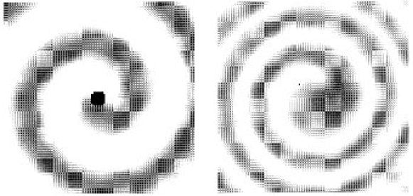
Figure 11: Spatial patterns of the limit cycle showing spiral waves around an initial obstacle (left) that was removed at later times (right). Courtesy of M.C. Boerlijst & P. Hogeweg [29].

These equations are in their nature similar to other chemical reaction-diffusion equations where several different substances catalyze each others reactions. A particularly exciting example is the famous Belousov-Zhabotinsky reaction, where malonic acid, CH₂(COOH)₂ is oxidized in the presence of bromate ions, BrO${}_{3}^{-}$. To initiate the reaction, cerium is used as catalyst to donate ions, although other metal ions are also possible. The color depends on the state of the cerium as it changes from Ce³⁺ to Ce⁴⁺ or, if iron is used, from Fe²⁺ to Fe³⁺. The resulting reactions are of the form [30]

$$A+Y\stackrel{{\scriptstyle k_{1}}}{{\longrightarrow}}X,$$ (38)

$$X+Y\stackrel{{\scriptstyle k_{2}}}{{\longrightarrow}}P,$$ (39)

$$B+X\stackrel{{\scriptstyle k_{3}}}{{\longrightarrow}}2X+Z,$$ (40)

$$2X\stackrel{{\scriptstyle k_{4}}}{{\longrightarrow}}Q,$$ (41)

$$Z\stackrel{{\scriptstyle k_{5}}}{{\longrightarrow}}Y,$$ (42)

where $X$=HBrO₂, $Y$=Br^-, $Z$=Ce⁴⁺, $A=B$=BrO${}_{3}^{-}$, $P$ and $Q$ are reaction products that do not contribute further to the reactions, and $k_{1},...,k_{5}$ are known rate constants. The reactions above lead to kinetic equations of the form

$${\partial[X]\over\partial t}=k_{1}[A][Y]-k_{2}[X][Y]+k_{3}[A][X]-k_{4}[X]^{2},$$ (43)

$${\partial[Y]\over\partial t}=-k_{1}[A][Y]-k_{2}[X][Y]+k_{5}[Z],$$ (44)

$${\partial[Z]\over\partial t}=2k_{3}[A][X]-k_{5}[Z].$$ (45)

This model of reaction equations is called the Oregonator, which refers to the affiliation of the authors at the time of publication [31].

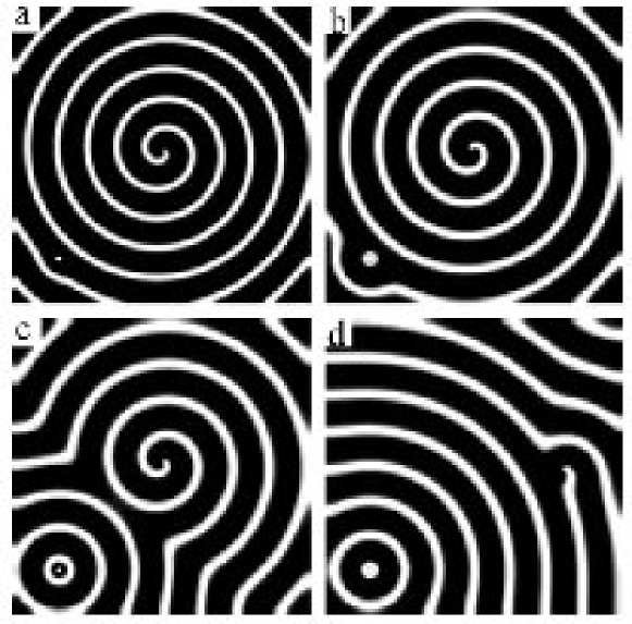
Figure 12: Spiral and ring-like patterns for the modified reaction equations by Zhang et al. [32]. On the boundaries a no-flux condition has been adopted, i.e. the normal components of all gradients vanish. Courtesy of X.Z. Zhang et al. [32].

If spatial extent is included via diffusion terms, this reaction exhibits in certain cases spiral patterns, similar to those in the model of Boerlijst & Hogeweg [28]. In Fig. 12 we reproduce the pattern obtained by Zhang et al. [32] for a slightly modified model consisting of only two partial differential equations. Depending on the value of a certain control parameter in their model spiral patterns of different size are being produced. An extensive review of the physics of pattern formation in different settings is given by Cross and Hohenberg [33].

The connection between pattern formation and the origin of life may seem rather remote. However, the equations governing chemical pattern formation illustrate some of the critical steps that are expected to play a role in origins of life. In particular the fact that different chemical compounds catalyze each other in a productive manner is an essential property behind the model proposed by Eigen. The Belousov-Zhabotinsky reaction also illustrates the phenomenon of autocatalysis where, in the presence of $A$, the molecule $X$ catalyzes the production of more $X$ by using $A$ as a substrate and producing $Z$ as additional side product.

The possibility of self-replication has been demonstrated for simple RNA molecules by Spiegelman [34] back in the late 1960s. There are now even examples of simple peptide chains that can catalyze the production of each other [35]. However, a serious shortcoming of any of the above examples discussed here is the fact that there is no possibility of natural selection and hence Darwinian evolution. So, as far as the question of the origin of life is concerned this pathway must be considered a dead end.

In summary one can say that there are similarities in the mathematics of producing homochirality and in establishing hereditary information in the composition of the first replicating polymers. However, in the latter case even less is known about the detailed nature of such polymers and their catalytic properties. A particularly important aspect is the possibility of spatial extent that can substantially modify the behavior of any chemical system. In the present case, as shown in Ref. [28], the possibility of spatial extent is critical for stabilizing the system against destruction by parasites. The model also exhibits spiral pattern formation that has been at the heart of the early work by Prigogine and others in connection with early ideas on biogenesis.

4 Alteration of the environment by early life

In this last section we discuss some physics problems within astrobiology that illustrate how life, once it has formed, might affect the environment of the early Earth and how it led to a planet so markedly different from a planet that does not harbor life.

4.1 Global energy balance of the Earth

The young Sun was about 30% fainter than today, and yet the young Earth was covered with liquid water and had temperatures higher than nowadays. This was caused by the presence of greenhouse gases such as water vapor, carbon dioxide, and probably also methane. Life is responsible for reducing $\mbox{CO}_{2}$ to compounds of the form $(\mbox{CH}_{2}\mbox{O})_{n}$ and similar, and to oxidize various minerals or to produce $\mbox{O}_{2}$. The resulting decrease of $\mbox{CO}_{2}$ weakens the greenhouse effect, so in this sense the emergence of life has essentially a cooling effect on the Earth’s overall climate.

Without atmosphere, the planet would cool like a black body at a rate proportional to the local flux $\sigma_{\rm SB}T^{4}$, where $\sigma_{\rm SB}$ is the Stefan-Boltzmann constant. Integrated over the entire surface of the planet, this corresponds to a loss of $4\pi R_{\rm E}^{2}\sigma_{\rm SB}T^{4}$, which would need to be balanced against the rate of energy received by solar radiation. The solar “constant” is $S=1.37\,{\rm kW}\,{\rm m}^{-2}$ and the total energy projected onto the disk of the Earth is $(1-A)\pi R_{\rm E}^{2}S$, where $A$ is the albedo, i.e. the fraction of energy reflected from the Earth. The resulting blackbody temperature would be

$$T_{0}=\left[(1-A){S\over 4\sigma_{\rm SB}}\right]^{1/4}.$$ (46)

Using $A=0.3$ and $\sigma_{\rm SB}=5.67\times 10^{-8}\,{\rm W}\,{\rm m}^{-2}\,{\rm K}^{-1})$, the temperature of the Earth would be $255\,{\rm K}$ or about $-18\,{\rm C}$.

In the presence of an atmosphere the rate of cooling is modified to $\sigma_{\rm SB}T_{\rm eff}^{4}$, where $T_{\rm eff}$ is the effective temperature equivalent to that of a black body. A positive greenhouse effect corresponds to $T_{\rm eff}<T$, so the cooling is reduced and the atmosphere heats up according to the vertically integrated energy equation

$$C{{\rm d}{}T_{0}\over{\rm d}{}t}=(1-A){S\over 4}-\sigma_{\rm SB}T_{\rm eff}^{4},$$ (47)

where $C$ is the vertically integrated specific heat.

The value of the effective temperature can be obtained from a radiative transfer calculation. A simplified model calculation yields

$$T_{\rm eff}^{4}={\ell\over\ell_{\rm crit}}\,T_{0}^{4},$$ (48)

where $T_{0}$ is the surface temperature, $\ell$ is an averaged mean free path of photons and $\ell_{\rm crit}$ is the critical value above which there is a positive greenhouse effect. Again, a simplified calculation suggests $\ell_{\rm crit}=3H/16\approx 0.19H$, where $H={\cal R}T/(\mu g)\approx 8\,{\rm km}$ is the pressure scale height of the atmosphere. So, an increase in opacity leads to a decrease of the cooling and hence to an increase in the surface temperature.

Another interpretation is to say that the greenhouse gases shift the radiating surface by a certain amount, $\ell_{\rm g}$, upward. The value of $\ell_{\rm g}$ is related to $\ell$. Ditlevsen [36] uses $\ell_{\rm g}=3\,{\rm km}$. He also noted that a more accurate lapse rate of the temperature is ${\rm d}{}T/{\rm d}{}z=10\,{\rm K}\,{\rm km}^{-1}$ instead of $T_{0}/H=40\,{\rm K}\,{\rm km}^{-1}$, so that the temperature gain caused by greenhouse gases is $\ell_{\rm g}\times{\rm d}{}T/{\rm d}{}z=30\,{\rm K}$. The reason for a shallower temperature gradient is the presence of convection that causes the specific entropy $s$ to be nearly constant with height. In that case the temperature gradient is just the adiabatic one, $({\rm d}{}T/{\rm d}{}z)_{\rm ad}=g/c_{p}$, where $c_{p}$ is the specific heat at fixed pressure, which in turn is related to the universal gas constant and the specific weight via ${\cal R}/\mu=c_{p}-c_{v}$, where $c_{v}$ is the specific heat at fixed volume and $c_{p}/c_{v}=\gamma$ is the ratio of specific heats. With these formulae one does indeed get

$$\left({{\rm d}{}T\over{\rm d}{}z}\right)_{\rm ad}=\left(1-{1\over\gamma}\right){\mu g\over{\cal R}}\approx 10\,{\rm K}\,{\rm km}^{-1},$$ (49)

where we have used $\gamma=7/5$ for air molecules with 5 degrees of freedom (3 for translation and 2 for rotation).

At certain times over the history of the Earth other greenhouse gases such as methane may have played an important role in keeping the Earth above freezing temperatures. Indeed, the burial of oxides in the crust allowed methane to build up in the atmosphere, which may have led to concentrations of a few thousand times greater than modern levels. UV radiation in the upper atmosphere breaks up methane into its components, letting H₂ to escape into space, leading to a net gain of oxygen, that comes ultimately from H₂O.

According to a model of Catling et al. [37] methane (CH₄) may have been important $2.7...2.3\,{\rm Gyr}$ ago, just before the famous Snowball Earth deep freeze of the Earth [38]. As discussed above, the associated loss of hydrogen may have led to a gradual accumulation of oxygen in the atmosphere, which then terminated the methane era and led to the Snowball Earth event. This event lasted until the continuous CO₂ production from volcanoes accumulated to large amounts so that the resulting greenhouse effect became sufficient to initiate partial melting of the ice cover.

4.2 Response to changes in greenhouse gases

As was known from global climate models [43] and later from simplified models [44] using Eq. (47) with a relatively simple piecewise linear temperature dependence of $A(T)$, there can be three different equilibrium temperatures. This is illustrated in Fig. 13, where we compare the graph of $\sigma_{\rm SB}T_{\rm eff}^{4}$ versus surface temperature $T_{0}$ with the net radiation $(1-A)S/4$. Here, $A(T)$ has been arranged such that $A=A_{\rm hot}$ for $T\geq T_{\max}$ (corresponding to no ice coverage) $A=A_{\rm cold}$ for $T\leq T_{\min}$ (corresponding to full ice coverage).

Ditlevsen [36] used Eq. (47) to study the response of the system to variable greenhouse gas concentrations. As the amount of CO₂ increases, the equilibrium temperature increases. Obviously, when the system was on the lower fixed point initially, there must be a critical CO₂ concentration above which the solution will jump discontinuously to the upper branch; see Fig. 14.

It is generally accepted that the rate of weathering increases with increasing temperature. This provides a stabilizing effect on the climate. As $T$ increases, the rate of weathering increases, removing more CO₂ from the atmosphere, reducing the greenhouse effect, and thus leading to cooling. Ditlevsen [36] introduced the assumption that there is a continuous source of CO₂ through outgassing from volcanoes and a temperature-dependent sink of CO₂ from weathering when $T$ exceeds a critical temperature $T_{\rm w}$, but no weathering for $T<T_{\rm w}$ [45]. This leads to a self-regulating effect for $T<T_{\rm w}$, which Ditlevsen calls a greenhouse thermostat. Whenever $T<T_{\rm w}$, since there is then no weathering and hence no sink of CO₂, greenhouse gases will build up until the Earth’s temperature has reached the value $T_{\rm w}$; see Fig. 15. This is the mechanism that is believed to have caused the early Earth to be above freezing through most of its history—with the exception of intermediate Snowball Earth-like events that are caused by the emergence of other sinks of greenhouse gases such as the onset of aerobic photosynthesis or the enhanced formation of mountain topography that leads to an increase in the erosion rate and hence the weathering.

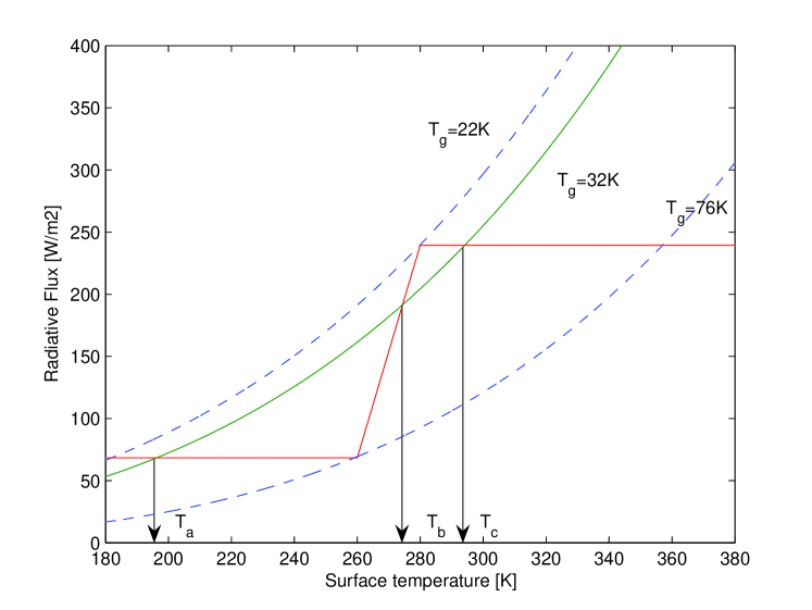
Figure 13: Plot of $\sigma_{\rm SB}T_{\rm eff}^{4}$ versus surface temperature $T_{0}$ for three different greenhouse temperature shifts, $T_{\rm g}$, compared with the net radiation ${\textstyle{1\over 4}}(1-A)$ for a simple piecewise linear function $A(T)$. Courtesy of P. Ditlevsen [36].

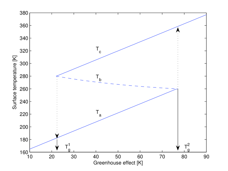
Figure 14: Equilibrium temperature as a function of CO₂ concentration. Courtesy of P. Ditlevsen [36].

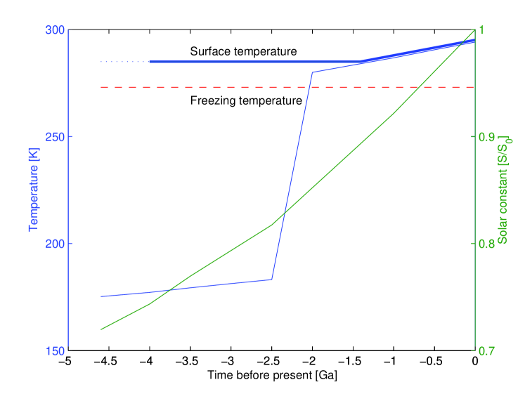
Figure 15: Dependence of surface temperature on time under the assumption of a continuous source of outgassing of CO₂ and the onset of a CO₂ sink for $T>T_{\rm w}$. Courtesy of P. Ditlevsen [36].

4.3 The Daisyworld model

Life can also affect the planet’s albedo, as has been demonstrated by Lovelock [39] in his Daisyworld model. For a tutorial on the Daisyworld model see Ref. [40]. This model also makes use of Eq. (47), but now the planet’s albedo $A$ is affected by the plant population which is simplistically represented by black and white plants or flowers (daisies) with local albedos $A_{1}$ and $A_{2}$, respectively. So the total albedo is a weighted average of the form

$$A=\sum_{i=1}^{3}\alpha_{i}A_{i},$$ (50)

where $A_{3}$ is the albedo of the unpopulated surface. The weights $\alpha_{i}$ depend on the surface coverage of the respective regions and obey evolution equations that are in turn governed by a temperature-dependent growth term, $\beta(T_{i})$, and a fixed death rate, $\gamma$, so the resulting equations for the rate of change of the albedo are

$${{\rm d}{}\alpha_{i}\over{\rm d}{}t}=[\beta(T_{i})-\gamma]\alpha_{i},$$ (51)

where $i=1$ for black and $i=2$ for white plant populations, $\beta(T)$ is assumed to be different from zero in the range $T_{\min}<T<T_{\max}$ with a maximum at $T_{\rm aver}={\textstyle{1\over 2}}(T_{\min}+T_{\max})$. The weight for the unpopulated surface follows from the normalization $\sum\alpha_{i}=1$, so $\alpha_{3}=1-\alpha_{1}-\alpha_{2}$.

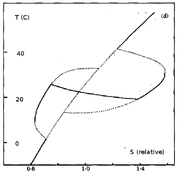
Figure 16: Temperature (in Celsius) versus relative irradiation (normalized to the average temperature). Note that the temperature is stabilized around the value $T_{\rm aver}$, provided the energy input $S$ is within a certain range. Courtesy of P.T. Saunders [42].

The temperatures are higher in the regions of black plants and lower in regions of white plants according to the formula

$$T_{i}^{4}=(A-A_{i})q+T_{0}^{4},$$ (52)

where $q$ is a parameter that must be smaller than a critical value,

$$q<q_{\rm crit}=S/(4\sigma_{\rm SB}),$$ (53)

in order that heat flows against the temperature gradient [42]. For $q=q_{\rm crit}$ the temperature is uniform for different values of $A_{i}$, while for $q<q_{\rm crit}$ the regions of high albedo are cooler and those of low albedo warmer. Note also that Eq. (52) preserves heat balance, i.e. $\sum\alpha_{i}T_{i}^{4}=T_{0}^{4}$.

The important point in the Daisyworld model is the fact that, for a certain range of $S$, the surface temperature of the planet, $T_{0}$, is stabilized to be in a certain temperature range around the optimal value close to $T_{\rm aver}$; see Fig. 16.

Saunders makes another remarkable point. He showed that by changing the model to allow for Darwinian evolution in such a way that each plant species works with an optimized temperature dependence, so $\beta(T_{i})\to\beta_{i}(T_{i})$ is modified to become dependent on $i$, the overall result changes only very little. More importantly, the range over which the model can stabilize the planet’s temperature shrinks, making the planet as a whole more vulnerable. Although the amount of shrinkage is small, it emphasizes the dangers associated with adopting changes that only lead to short-term benefits. Saunders emphasizes in his work that the ability of life to regulate the surface temperature of a planet is not associated with natural selection as in the concept of Darwinian evolution. More generally he warns therefore that not everything that is to an advantage needs to be the result of natural selection [42].

4.4 Oxidation of the Earth’s crust

It has recently been proposed that, in addition to the effects discussed above, life may have profound effects also on the Earth’s crust. A possible scenario of such a suggestion has recently been discussed by Rosing et al. [46]. The idea is that photosynthetic life may tap large amounts of solar energy that were used to reduce carbon from $\mbox{CO}_{2}$ to compounds of the form $(\mbox{CH}_{2}\mbox{O})_{n}$ and similar, via reactions of the form

$$\mbox{CO}_{2}+\mbox{H}_{2}\mbox{O}+h\nu\rightarrow\mbox{CH}_{2}\mbox{O}+\mbox{O}_{2},$$ (54)

where $h\nu$ denotes the energy taken from solar radiation. Furthermore, and even more surprisingly, the oxygen produced by photosynthesis may have been critical in oxidizing iron in the continental crust. Although other factors also plaid a substantial role, it is clear that biological processes can speed up the oxidation process substantially. Comparing the oceanic crust with continental crust, a major difference is the enhanced fraction of SiO₂ (57% in the continental crust compared to 50% in the oceanic crust).

With granite being one of the lightest rock types, it was eventually able to escape subduction and to produce stable continents about $3.8\,{\rm Gyr}$ ago. This is also the time of the oldest rock findings on Earth. Given that the rise of continents on the early Earth is associated with granite formation, the presence of granite on silicon-bearing rocky planets might thus be a possible biomarker for photosynthesis [46].

Although this idea is speculative, it may be supported quantitatively as follows. Firstly, the present day production rate of organically fixated carbon is estimated to be $9\times 10^{15}\,{\rm mol}\,\mbox{C}\,{\rm yr}^{-1}$ [47, 48]. The amount of energy required for this can be calculated by using the fact that it costs $477\,{\rm kJ}$ to transfer one mol carbon to hexose. The energy required for this is then $300\,{\rm mW}\,{\rm m}^{-2}$. Rosing et al. [46] argue that this amount could be supplied by only 0.1% of the effective solar energy flux, $S/4$. Assuming that the amount of carbon burial, relevant to estimating the usable fraction of oxygen for iron oxidation, is also about $0.1\%$, this corresponds to about $10^{13}\,{\rm mol}\;\mbox{C}\,{\rm yr}^{-1}$. This would yield a comparable iron oxidation rate. Rosing et al. [46] argue further that the annual basalt production contributes about $10^{14}\,{\rm mol}\;\mbox{Fe}\,{\rm yr}^{-1}$, so a fraction of the magmatic iron flux could be used for building up the mantle reservoir of ferric iron.

In conclusion, the presence of life can lead to significant alterations of the planet in a number of different ways, as is quite clearly demonstrated by some of the differences between Earth and its neighboring planets Venus and Mars. Only the Earth has extensive reservoirs of oxygen and of granite. Within limits, the presence of life on a planet can also have a stabilizing effect on its climate. The relevant mathematical modeling of some of these processes resembles in many ways those encountered earlier in studies of homochirality and of the spread of hereditary information on the early Earth.

5 Conclusions

Astrobiology has developed into a rapidly growing research field involving expertise from a number of neighboring disciplines. Nonlinear dynamics and nonequilibrium thermodynamics find applications in all these subfields. Here, we have elaborated on a few such aspects. Closest to the onset of life is perhaps the emergence of homochirality of biomolecules. Given that RNA has been proven to form longer polymers only in a homochiral environment, one would expect that homochirality must be a prerequisite to the emergence of life at the level of a replicating RNA world. On the other hand, the very mechanism causing the polymerization to terminate, namely the enantiomeric cross-inhibition, can also be the mechanism responsible for causing 100% homochirality by destroying RNA molecules whose chirality is already in the minority. This would however requite the possibility of auto-catalysis, which can be avoided in another scenario where a closed peptide system is kept away from equilibrium by continuous activation of amino acids.

Chemically speaking, the stabilization of a definite chirality is in some models similar to the subsequent establishment of hereditary information in that catalysis plays a crucial role. Furthermore, in both cases the possibility of chemistry in an extended system is crucial. On the one hand, spatial extent gives rise to the possibility of coexistence of life forms of opposite handedness on the early Earth. On the other hand, spatial extent can be critical in allowing the system to find unpopulated locations faster than being overwhelmed by the effects of parasites that tap the same resources that are required for the maintenance and development of hereditary information.

Finally, life is invariably coupled to come kind of metabolism that is ultimately powered by solar energy. This clearly affects the environment by reducing carbon and oxidizing the crust of the Earth and, over the last two billion years also the atmosphere. How much these alterations of the environment are due to biological processes is less obvious. However, it is clear that biological factors greatly speed up weathering on the Earth. The extent of biologically induced alterations of the continental crust, for example, may therefore best be tested using quantitatively accurate model calculations. The outcome may ultimately hinge on energetic considerations and on the efficiency of photosynthesis as a solar energy collector.

With the scope of being able to explore in the near future not only the planets and other celestial bodies in the solar system in much more detail, but also planets of other planetary systems, the research in astrobiology quickly develops into a field that will be driven more and more by new data, making this field less susceptible to speculation. It is therefore important to be prepared for upcoming discoveries in this field. Finally, it should be emphasized that astrobiology is efficient in communicating science to the general public, which may provide additional boost to the field.

Additional reading

• Barbieri M (2003) The organic codes: an introduction to semantic biology, Cambridge: CUP.

  Brack A (1998) The molecular origins of life, Cambridge University Press, Cambridge.

  Darwin C (1859) The origin of species by means of natural section, Reprinted by Penguin books, London 1985.

  Haken H (1983) Synergetics – An Introduction, Springer, Berlin.

  Lovelock JE (1995) Gaia. A new look at life on Earth, Oxford Univ. Press, Oxford.

  Lunine J (2003) Astrobiology: a multi-disciplinary approach, Pearson Addison-Wesley, San Franciso.

  Prigogine I (1980) From being to becoming. Time and complexity in the physical sciences, Freeman, New York.

  Rauchfuß H (2005) Chemische Evolution und der Ursprung des Lebens, Springer, Berlin.

  Ward PD, Brownlee D (2000) Rare Earth: why complex life is uncommon in the Universe, Copernicus, Springer: New York.

$Header: /var/cvs/brandenb/tex/bio/encyc/paper.tex,v 1.39 2007/08/12 21:43:21 brandenb Exp $

References

- [1] Davies PCW, Lineweaver CH (2005) Finding a second sample of life on Earth, Astrobiol. 5, 154–163.
- [2] Rasmussen S, Chen L, Nilsson M, Abe S (2003) Bridging nonliving and living matter, Artif Life 9, 269–316.
- [3] Turing AM (1952) The chemical basis of morphogenesis, Phil. Trans. Roy. Soc. B237, 37–72.
- [4] Prigogine I, Nicolis G (1967) On symmetry-breaking instabilities in dissipative systems , J Chem Phys 46, 3542–3550.
- [5] Prigogine I, Lefever R (1968) Symmetry breaking instabilities in dissipative systems II, J Chem Phys 48, 1695–1700.
- [6] Eigen M (1971) Selforganization of matter and evolution of biological macromolecules, Naturwissenschaften 58, 465–523.
- [7] Gilbert W (1986) Origin of life – the RNA world, Nature 319, 618–618.
- [8] Nielsen PE (1993) Peptide nucleic acid (PNA): A model structure for the primordial genetic material, Orig. Life Evol. Biosph. 23, 323–327.
- [9] Russell M (2006) First life, Am Sci 94, 32–39.
- [10] Lathe R (2004) Fast tidal cycling and the origin of life, Icarus 168, 18–22.
- [11] Bywater RP, Conde-Frieboesk K (2005) Did Life Begin on the Beach? Astrobiol. 5, 568–574.
- [12] Miller SL (1953) A production of amino acids under possible primitive Earth conditions, Science 117, 528–529.
- [13] Plasson R, Kondepudi DK, Bersini H, Commeyras A, Asakura K (2007) Emergence of homochirality in far-from-equilibrium systems: Mechanisms and role in prebiotic chemistry, Chirality 19, 589–600.
- [14] Joyce GF, Visser GM, van Boeckel CAA, van Boom JH, Orgel LE, Westrenen J (1984) Chiral selection in poly(C)-directed synthesis of oligo(G), Nature 310, 602–603.
- [15] Frank FC (1953) On spontaneous asymmetric synthesis, Biochim Biophys Acta 11, 459–464.
- [16] Blackmond DG (2004) Asymmetric autocatalysis and its implications for the origin of homochirality, Proc. Natl. Acad. Sci. 101, 5732–5736.
- [17] Soai K, Shibata T, Morioka H, Choji K (1995) Asymmetric autocatalysis and amplification of enantiomeric excess of a chiral molecule, Nature 378, 767–768.
- [18] Sandars PGH (2003) A toy model for the generation of homochirality during polymerization, Orig. Life Evol. Biosph. 33, 575–587.
- [19] Brandenburg A, Andersen AC, Höfner S, Nilsson M (2005) Homochiral growth through enantiomeric cross-inhibition, Orig. Life Evol. Biosph. 35, 225–241.
- [20] Murray JD (2002) Mathematical Biology. An introduction, Springer, New York.
- [21] Brandenburg A, Multamäki T (2004) How long can left and right handed life forms coexist? Int. J. Astrobiol. 3 209–219.
- [22] Shibata R, Saito Y, Hyuga H (2006) Diffusion accelerates and enhances chirality selection, Phys. Rev. E 74, 026117.
- [23] Plasson R, Bersini H, Commeyras A (2004) Recycling Frank: spontaneous emergence of homochirality in noncatalytic systems, Proc. Natl. Acad. Sci. 101, 16733–16738.
- [24] Brandenburg, A., Lehto, H. J., & Lehto, K. M. (2007) Homochirality in an early peptide world, Astrobiol. 7, 725–732.
- [25] Eigen M (2002) Error catastrophe and antiviral strategy, Proc. Natl. Acad. Sci. 99, 13374–13376.
- [26] Dyson FJ (1999) Origins of life, Cambridge University Press, Cambridge.
- [27] Eigen M, Schuster P (1977) The hypercycle, Naturwissenschaften 64, 541–565.
- [28] Boerlijst MC, Hogeweg P (1991) Spiral wave structure in pre-biotic evolution - hypercycles stable against parasites, Physica D 48, 17–28.
- [29] Boerlijst MC, Hogeweg P (1995) Attractors and spatial patterns in hypercycles with negative interactions, J Theor Biol 176, 199–210.
- [30] Murray JD (1974) On a model for the temporal oscillations in the Belousov–Zhabotinsky reaction, J Chem Phys 61, 3610–3613.
- [31] Field RJ, Körö E, Noyes RM (1972) Oscillations in chemical systems, part 2. Thorough analysis of temporal oscillations in the bromate-cerium-malonic acid system, J Am Chem Soc 94, 8649–8664.
- [32] Zhang XZ, Liao HM, Zhou LQ, Quyang Q (2004) Pattern selection in the Belousov–Zhabotinsky reaction with the addition of an activating reactant, J Phys Chem B 108, 16990–16994.
- [33] Cross MC, Hohenberg PC (1993) Pattern formation outside of equilibrium, Rev. Mod. Phys. 65, 851–1112.
- [34] Mills DR, Peterson RL, Spiegelman S (1967) An extracellular Darwinian experiment with a self-duplicating nucleic acid molecule, Proc. Natl. Acad. Sci. 58, 217–224.
- [35] Saghatelian A, Yokobayashi Y, Soltani K, Ghadiri MR (2001) A chiroselective peptide replicator, Nature 409, 797–801.
- [36] Ditlevsen PD (2005) A climatic thermostat making Earth habitable, Int. J. Astrobiol. 4, 3–7.
- [37] Catling DD, Zahnle KJ, McKay CP (2001) Biogenic methane, hydrogen escape, and the irreversible oxidation of early Earth, Science 293, 839–843.
- [38] Hoffman PF, Kaufman AJ, Halverson GP, Schrag DP (1998) A Neoproterozoic Snowball Earth, Science 281, 1342–1346.
- [39] Watson AJ, Lovelock JE (1983) Biological homeostasis of the global environment: the parable of Daisyworld, Tellus B 35, 284–289.
- [40] von Bloh W, Block A, Parade M, Schellnhuber HJ (1999) Tutorial Modelling of geosphere-biosphere interactions: the effect of percolation-type habitat fragmentation, Physica A 266, 186–106.
- [41] Taylor FW (1991) The greenhouse effect and climate change, Rep. Prog. Phys. 54, 881–918.
- [42] Saunders PT (1994) Evolution without natural selection: further implications of the Daisyworld parable, J Theor Biol 166, 365–373.
- [43] Ghil M (1976) Climate stability for a Sellers-type model, J. Atmos. Sci. 33, 3–20.
- [44] Crafoord C, Källén E (1978) A note on the condition for existence of more than one steady-state solution in Budyko-Sellers type models, J. Atmos. Sci. 35, 1123–1125.
- [45] Walker JCG, Hays PB, Kasting JF (1981) A negative feedback mechanism for the long-term stabilization of the Earth’s surface temperature, J. Geophys. Res. 86, 9776–9782.
- [46] Rosing MT, Bird DK, Sleep NH, Glassley, W., Albarede, F. (2006) The rise of continents–An essay on the geologic consequences of photosynthesis, Palaeogeogr, Palaeoclimatol, Palaeoecol 232, 99–113.
- [47] Martin JH, Knauer GA, Karl DM, Broenkow WW (1987) Vertex - carbon cycling in the Northeast Pacific, Deep-Sea Res Part A 34, 267–285.
- [48] Des Marais DJ (2000) When did photosynthesis emerge on Earth, Science 289, 1703–1705.