$B\!\to\!\!D^{(*)}$ Form Factors
from QCD Light-Cone Sum Rules
S. Faller ^(a,b), A. Khodjamirian ^(a), Ch. Klein ^(a) and Th. Mannel ^(a)
(a) Theoretische Physik 1, Fachbereich Physik, Universität Siegen,
D-57068 Siegen, Germany
^(b)  Theory Division, Department of Physics, CERN,
CH-1211 Geneva 23, Switzerland

We derive new QCD sum rules for $B\to D$ and $B\to D^{*}$ form factors. The underlying correlation functions are expanded near the light-cone in terms of $B$-meson distribution amplitudes defined in HQET, whereas the $c$-quark mass is kept finite. The leading-order contributions of two- and three-particle distribution amplitudes are taken into account. From the resulting light-cone sum rules we calculate all $B\to D^{(*)}$ form factors in the region of small momentum transfer (maximal recoil). In the infinite heavy-quark mass limit the sum rules reduce to a single expression for the Isgur-Wise function. We compare our predictions with the form factors extracted from experimental $B\to D^{(*)}l\nu_{l}$ decay rates fitted to dispersive parameterizations.

1 Introduction

The hadronic form factors of $B\!\to\!D,D^{*}$ transitions are used to extract the CKM parameter $V_{cb}$ from the measurements of the semileptonic $B\to D^{(*)}l\nu_{l}$ decay rates. These form factors were among the first and most important applications of the heavy quark symmetry [1, 2] and heavy quark effective theory (HQET)[3] (for reviews see [4, 5, 6]).

In the heavy-quark limit, all $B\!\to\!D^{(*)}$ form factors are expressed via the Isgur-Wise (IW) function $\xi(w)$ of the velocity transfer $w=v\cdot v^{\prime}$ in the $B(v)\!\to\!D^{(*)}(v^{\prime})$ transition. The gluon radiative and inverse heavy-mass corrections are well understood within heavy-quark expansion and HQET (see e.g., [4, 6, 7]), in particular at the zero recoil ($w=1$) point. The $B\!\to\!D^{(*)}$ form factors are also being calculated in lattice QCD [8, 9, 10]. Beyond the zero-recoil point, at $w>1$, one usually parameterizes these form factors [11, 12], employing conformal mapping and dispersive bounds based on analyticity and unitarity. The data on $B\to D^{(*)}l\nu_{l}$, including the most recent measurements [13, 14] are fitted to these parameterizations.

For a better theoretical description of $B\to D^{(*)}l\nu_{l}$ transitions in the whole kinematical region and for a quantitative assessment of $1/m_{Q}$ corrections it is desirable to perform alternative calculations of the form factors within full QCD, with finite heavy quark masses, at least, with a finite $c$-quark mass. Previously, $B\to D^{(*)}$ form factors were calculated from QCD sum rules for three-point correlation functions with finite $b$- and $c$-quark masses [15, 16]. These calculations employ the local operator-product expansion (OPE) and include nonperturbative effects in the form of quark and gluon condensates. Based on double dispersion relations, the three-point sum rules are quite sensitive to the choice of the quark-hadron duality region. The heavy-quark limit of three-point sum rules reproduces a universal IW function and reveals noticeable corrections from finite quark masses (see e.g.,[16]) . A direct calculation of the IW function from the sum rules in HQET is also possible [17, 18, 19, 20], including $O(\alpha_{s})$ corrections [21].

A well known alternative sum rule approach to hadronic form factors relies on the OPE near the light-cone [22] and employs the light-cone distribution amplitudes of hadrons. This approach has been successfully applied to heavy-light form factors (some recent results can be found in [23, 24, 25, 26, 27]). It is timely to develop a similar technique also for the $B\to D^{(*)}$ form factors.

In this paper we apply the recently suggested version of QCD light-cone sum rules [24, 25], in which the set of $B$-meson distribution amplitudes (DA’s) serves as a universal nonperturbative input (in [26] a similar approach was used in the framework of SCET). We keep the $c$-quark mass finite and employ the quark-hadron duality approximation in the $D^{(*)}$ channel of the correlation function. The on-shell $B$ meson is treated in HQET, to allow the expansion in DA’s. As discussed below, the light-cone expansion is applicable in the region of maximal recoil. We obtain predictions for all $B\to D^{(*)}$ form factors in this region and compare the results with the experimental data on semileptonic decay rates. We also derive the infinite heavy-quark mass limit of the new sum rules.

The plan of the paper is as follows. In section 2 we introduce the correlation function and derive the sum rules for the form factors. In section 3 we switch to the form factors adapted to heavy-quark symmetry and discuss the heavy-mass limit of the sum rules. Section 4 is devoted to numerical results. In section 5 we conclude. The appendix contains definitions of $B$-meson DA’s and the bulky expressions for three-particle contributions to sum rules.

2 Correlation function and sum rules

Following [25], we consider the correlation function of two quark currents taken between the vacuum and the on-shell $\bar{B}$-meson state:

$$F_{a\mu}^{(B)}(p,q)=i\int d^{4}x~{}e^{ip\cdot x}\langle 0|T\left\{\bar{d}(x)\Gamma_{a}c(x),\bar{c}(0)\gamma_{\mu}(1-\gamma_{5})b(0)\right\}|\bar{B}(p_{B})\rangle\,,$$ (1)

where the weak $b\to c$ current is correlated with the $\bar{d}(x)\Gamma_{a}c(x)$ current. The latter interpolates the pseudoscalar $D$-meson ($\Gamma_{a}=m_{c}i\gamma_{5}$) or vector $D^{*}$-meson ($\Gamma_{a}=\gamma_{\nu}$). For definiteness, we choose the $\bar{B}_{d}\to D^{(*)+}$ transition, equivalent to $\bar{B}_{u}\to D^{(*)0}$ in the isospin symmetry limit. The external momenta of the weak and interpolating currents are $q$ and $p$, respectively, with the $B$ meson momentum being on-shell, $p_{B}^{2}=(p+q)^{2}=m_{B}^{2}$ .

The correlation function (1) is related to the form factors of our interest via the hadronic dispersion relation in the channel of the charmed meson:

$$F_{a\mu}^{(B)}(p,q)=\frac{\langle 0|\bar{d}\Gamma_{a}c|D^{(*)}(p)\rangle\langle D^{(*)}(p)|\bar{c}\gamma_{\mu}(1-\gamma_{5})b|\bar{B}(p+q)\rangle}{m_{D^{(*)}}^{2}-p^{2}}+...\,,$$ (2)

where the $D^{(*)}$-meson pole term is shown explicitly, and ellipses indicate the contributions of excited and continuum states. The r.h.s. of Eq. (2) contains the decay constant:

$$\langle 0|\bar{d}m_{c}i\gamma_{5}c|D(p)\rangle=m_{D}^{2}f_{D},$$ (3)

or

$$\langle 0|\bar{d}\gamma_{\nu}c|D^{*}(p,\epsilon)\rangle=\epsilon_{\nu}m_{D^{*}}f_{D^{*}}\,,$$ (4)

(where $\epsilon$ is the polarization vector of $D^{*}$) and the $B\to D^{(*)}$ transition matrix element. The latter is determined by the form factors for which we use the standard definitions:

$$\langle D(p)|\bar{c}\gamma_{\mu}b|\bar{B}(p+q)\rangle=2p_{\mu}f^{+}_{BD}(q^{2})+q_{\mu}\left[f^{+}_{BD}(q^{2})+f^{-}_{BD}(q^{2})\right]\,,$$ (5)

and

$$\langle D^{*}(p,\epsilon)|\bar{c}\gamma_{\mu}(1-\gamma_{5})b|\bar{B}(p+q)\rangle=-i\epsilon_{\mu}^{*}(m_{B}+m_{D^{*}})A_{1}^{BD^{*}}(q^{2})$$

$$+i(2p+q)_{\mu}(\epsilon^{*}q)\dfrac{A_{2}^{BD^{*}}(q^{2})}{m_{B}+m_{D}{{}^{*}}}+iq_{\mu}(\epsilon^{*}q)\dfrac{2m_{D^{*}}}{q^{2}}\Big{(}A_{3}^{BD^{*}}(q^{2})-A_{0}^{BD^{*}}(q^{2})\Big{)}$$

$$+\epsilon_{\mu\nu\rho\sigma}\epsilon^{*\nu}q^{\rho}p^{\sigma}\dfrac{2V^{BD^{*}}(q^{2})}{m_{B}+m_{D^{*}}}\,,$$ (6)

where $A_{0}^{BD^{*}}(0)=A_{3}^{BD^{*}}(0)$ and

$$2m_{D}^{*}A_{3}^{BD^{*}}(q^{2})=(m_{B}+m_{D^{*}})A_{1}^{BD^{*}}(q^{2})-(m_{B}-m_{D^{*}})A_{2}^{BD^{*}}(q^{2})\,.$$

The sum rule derivation follows the procedure similar to the one applied in [25]. Instead of the virtual light quark now the $c$ quark propagates in the correlation function. The calculation is performed in terms of $B$-meson DA’s defined in HQET, hence the correlation function (1) has to be expanded in the limit of large $m_{b}$:

$$F_{a\mu}^{(B)}(p,q)=\tilde{F}_{a\mu}^{(B_{v})}(p,q^{\prime})+O(1/m_{b})\,,$$ (7)

where the limiting correlation function is

$$\tilde{F}_{a\mu}^{(B_{v})}(p,q^{\prime})=i\int d^{4}x~{}e^{ip\cdot x}\langle 0|T\left\{\bar{d}(x)\Gamma_{a}c(x),\bar{c}(0)\gamma_{\mu}(1-\gamma_{5})h_{v}(0)\right\}|\bar{B}_{v}\rangle\,.$$ (8)

and each term of this expansion retains dependence on finite $m_{c}$. In the above, the four-momentum of the $B$-meson state is redefined as $p_{B}=m_{b}v+k$, where $v$ is the four-velocity of $B$, $k$ is the residual momentum, and the relativistic normalization of the state $|\bar{B}(p_{B})\rangle=|\bar{B}_{v}\rangle$ (up to $1/m_{b}$ corrections) is retained. In addition, the $b$-quark field is substituted by the effective field, using $b(x)=h_{v}(x)e^{-im_{b}vx}+O(1/m_{b})$, and the four-momentum transfer $q$ is redefined by separating the “static” part of it: $q=m_{b}v+q^{\prime}$. In what follows, the initial correlation function (1) is calculated in the approximation (8). Note that (8) does not depend on $m_{b}$ since the external momentum scales $p$ and $q^{\prime}$ are generic and do not scale with the heavy quark mass.

Before turning to the calculation, it is important to convince oneself that the light-cone dominance is valid for off-shell external momenta $p$ and $q$, that is, if $p^{2}$ and $q^{2}$ are far below the hadronic thresholds in the channels of $\bar{d}\Gamma_{a}c$ and $\bar{c}\gamma_{\mu}(1-\gamma_{5})b$ currents, respectively. To demonstrate that, we can use the same line of arguments as in [25]. For simplicity, we consider the rest frame $v=(1,0,0,0)$, where, in first approximation, $m_{B}=m_{b}+\bar{\Lambda}$, so that $k_{0}\sim\bar{\Lambda}$. In addition, it is also convenient to rescale the $c$-quark field by introducing an effective field $h^{\prime}_{v}(x)=c(x)e^{-im_{c}vx}$ (with the same velocity). Simultaneously, the external four-momenta are redefined: $p=m_{c}v+\tilde{p}$, $q^{\prime}=-m_{c}v+\tilde{q}$, separating the parts proportional to the velocity $v$, so that $q=(m_{b}-m_{c})v+\tilde{q}$, and $\tilde{p}+\tilde{q}=k$. Note that the last redefinitions do not necessarily mean that we will use HQET also for the virtual $c$-quark field. It is done only in order to decouple the $c$-quark mass scale. Indeed, we now arrive at a modified correlation function

$$\tilde{F}_{a\mu}^{(B_{v})}(\tilde{p},\tilde{q})=i\int d^{4}x~{}e^{i\tilde{p}\cdot x}\langle 0|T\left\{\bar{d}(x)\Gamma_{a}h^{\prime}_{v}(x),\bar{h}_{v}^{\prime}(0)\gamma_{\mu}(1-\gamma_{5})h_{v}(0)\right\}|\bar{B}_{v}\rangle$$ (9)

of two effective currents with the external momenta $\tilde{p}$, $\tilde{q}$. This correlation function does not explicitly depend on both $b$- and $c$- quark masses and contains only the scales associated with either effective or light-quark degrees of freedom.

We assume that both rescaled four-momenta are spacelike and their squares are sufficiently large:

$$P^{2},|\tilde{q}^{2}|\gg\Lambda_{QCD}^{2},\bar{\Lambda}^{2}\,,$$ (10)

where $P^{2}=-\tilde{p}^{2}$. Furthermore, the difference between the virtualities is also kept large, so that the ratio

$$\zeta=\frac{2\tilde{p}\cdot k}{P^{2}}\sim\frac{|\tilde{q}^{2}|-P^{2}}{P^{2}}\sim 1\,.$$ (11)

With these two conditions fulfilled, the region of small $x^{2}\leq 1/P^{2}$ dominates in the integral in (9), in full analogy with the $\gamma^{*}(\tilde{p})\gamma^{*}(\tilde{q})\to\pi^{0}(\tilde{p}+\tilde{q})$ transition amplitude, for which a detailed proof of the light-cone dominance can be found e.g., in [28]. Thus, the choice of large $P^{2}$ and $\zeta\sim 1$ enables the validity of light-cone OPE. In terms of the initial external momenta $p$ and $q$, one now has

$$p^{2} = m_{c}^{2}-\zeta m_{c}P^{2}/\bar{\Lambda}-P^{2}\,,$$

$$q^{2} = (m_{b}-m_{c})^{2}-(m_{b}-m_{c})P^{2}\zeta(1+\zeta)/\bar{\Lambda}-P^{2}(1+\zeta)\,,$$ (12)

taking into account that $\tilde{p}_{0}=\zeta P^{2}/(2\bar{\Lambda})$ in the rest frame. Note that the external momentum squared $p^{2}$ in the charmed meson channel has to be shifted below the threshold $m_{D^{(*)}}^{2}\sim m_{c}^{2}$ by an interval $\sim m_{c}\chi$. The scale $\chi\sim P^{2}/\bar{\Lambda}\gg\bar{\Lambda},\Lambda_{QCD}$ is large in terms of$\Lambda_{QCD}$ , but in general independent of the heavy quark masses. The situation here is quite similar to the correlation function used to derive LCSR for $B\to\pi$ form factors with pion DA’s (see e.g.,[23, 27]), in which case the light-cone dominance is guaranteed by off-shell external momenta. Importantly, the second condition in (12) tells us that OPE is only applicable sufficiently far from the zero recoil (maximal $q^{2}$) point $q^{2}=(m_{B}-m_{D}^{(*)})^{2}\sim(m_{b}-m_{c})^{2}$ of the $B\to D^{(*)}$ transition. In practice, LCSR will be applied at $q^{2}\sim 0$, near the maximal recoil. Solving the second equation in (12) for $q^{2}=0$ we obtain $P^{2}\sim\bar{\Lambda}(m_{b}-m_{c})\ll m_{b}^{2}$, however, the components of the external momenta reach the order of magnitude of the heavy-quark mass scale.

Returning to the correlation function (8), we calculate the leading order (LO) contributions of two- and three-particle $B$-meson DA’s. The corresponding diagrams are depicted in Figs. 1a and 1b, respectively. We use the $c$-quark propagator near the light-cone, including the one-gluon part [29]:

$$S_{c}(x,0)=-i\langle 0|T\{c(x)\bar{c}(0)\}|0\rangle=\!\int\!\dfrac{d^{4}p}{(2\pi)^{4}}e^{-ipx}\Bigg{\{}\dfrac{\mathchoice{\ooalign{$\hfil\displaystyle\mkern 0.0mu/\hfil$\crcr$\displaystyle p\,$}}{\ooalign{$\hfil\textstyle\mkern 0.0mu/\hfil$\crcr$\textstyle p\,$}}{\ooalign{$\hfil\scriptstyle\mkern 0.0mu/\hfil$\crcr$\scriptstyle p\,$}}{\ooalign{$\hfil\scriptscriptstyle\mkern 0.0mu/\hfil$\crcr$\scriptscriptstyle p\,$}}\>\!+m_{c}}{p^{2}-m_{c}^{2}}$$ (21)

$$+\!\int_{0}^{1}\!d\alpha\,G_{\mu\nu}(\alpha x)\left[\dfrac{\alpha x^{\mu}\gamma^{\nu}\,}{p^{2}-m_{c}^{2}}-\dfrac{(\mathchoice{\ooalign{$\hfil\displaystyle\mkern 0.0mu/\hfil$\crcr$\displaystyle p\,$}}{\ooalign{$\hfil\textstyle\mkern 0.0mu/\hfil$\crcr$\textstyle p\,$}}{\ooalign{$\hfil\scriptstyle\mkern 0.0mu/\hfil$\crcr$\scriptstyle p\,$}}{\ooalign{$\hfil\scriptscriptstyle\mkern 0.0mu/\hfil$\crcr$\scriptscriptstyle p\,$}}\>\!+m_{c})\sigma^{\mu\nu}}{2(p^{2}-m_{c}^{2})^{2}}\right]\Bigg{\}}\,,$$ (30)

where $G_{\mu\nu}=g_{s}G^{a}_{\mu\nu}(\lambda^{a}/2)$. Calculating the correlation function, we confine ourselves by the zeroth order in $\alpha_{s}$, hence the $O(\alpha_{s})$ differences between various $c$-quark mass definitions are beyond our accuracy. Generally, since there is a highly virtual $c$-quark in the correlation function, (and in anticipation of future $O(\alpha_{s})$ corrections to LCSR), the most natural choice is the $\overline{MS}$ mass, which we adopt in numerical calculations.

After contracting $c$-quark fields and substituting the propagator (30) the correlation function is expressed in terms of two- and three-particle DA’s of the $B$-meson. Their definitions are given in the Appendix, where we also specify the adopted exponential model of two-particle DA’s suggested in [30] and the corresponding set of three-particle DA’s derived in [25] from QCD sum rules in HQET.

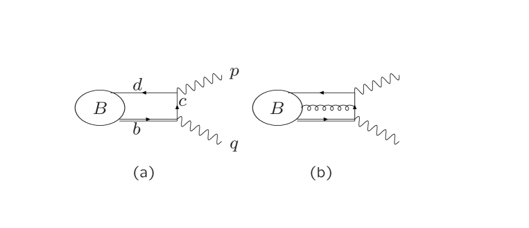
Figure 1: Diagrams corresponding to the contributions of (a) two-particle and (b) three-particle $B$-meson DA’s to the correlation function (1); Curly (wavy) lines denote gluons (external currents).

The result for the correlation function is equated to the hadronic representation (2). Each independent Lorentz-structure in this equation provides a sum rule relation for a certain form factor or a combination of form factors. In the correlation function for $B\to D$ form factors we take the coefficients at $p_{\mu}$ and $q_{\mu}$ to obtain the sum rules for the form factors $f^{+}_{BD}$ and $f^{+}_{BD}+f^{-}_{BD}$, respectively. In the $B\to D^{*}$ case, we choose the kinematical structures $\epsilon_{\mu\nu\rho\sigma}q^{\rho}p^{\sigma}$, $g_{\mu\nu}$ and $p_{\mu}q_{\nu}$ for the form factors $V^{BD^{*}}$, $A_{1}^{BD^{*}}$ and $A_{2}^{BD^{*}}$, respectively. To obtain the sum rule for the remaining combination of form factors $A_{3}^{BD^{*}}-A_{0}^{BD^{*}}$, the sum rule for the invariant amplitude multiplying $q_{\mu}q_{\nu}$ in the correlation function has to be derived, from which the sum rule for $A_{2}^{BD^{*}}$ has to be subtracted. The further derivation of the sum rules does not differ from the procedure explained in [25] and we will not repeat the details here.

First, we present the sum rules for the two $B\to D$ form factors:

$$f^{+}_{BD}(q^{2})=\frac{\text{fB}m_{B}m_{c}}{2\text{fD}m_{D}^{2}}\Bigg{\{}\int\limits_{0}^{\omega_{0}(q^{2},\text{s0D})}d\omega\exp\left(\frac{-s(\omega,q^{2})+m_{D}^{2}}{\text{M2}}\right)\\ \times\left[\frac{m_{c}(\overline{\omega}+m_{c})}{\overline{\omega}^{2}+m_{c}^{2}-q^{2}}\text{phiBmin}(\omega)+(\overline{\omega}+m_{c})\left(\frac{1}{\overline{\omega}}-\frac{m_{c}}{\overline{\omega}^{2}+m_{c}^{2}-q^{2}}\right)\text{phiBp}(\omega)\right.\\ \left.-\left(\frac{1}{\overline{\omega}}+\frac{m_{c}(\overline{\omega}^{2}+2m_{c}\overline{\omega}-m_{c}^{2}+q^{2})}{\left(\overline{\omega}^{2}+m_{c}^{2}-q^{2}\right)^{2}}\right)\text{PhiBpm}(\omega)\right]+\Delta f^{+}_{BD}(q^{2},s_{0}^{D},M^{2})\Bigg{\}}\,,$$ (31)

$$f^{+}_{BD}(q^{2})+f^{-}_{BD}(q^{2})=-\frac{\text{fB}m_{B}m_{c}}{\text{fD}m_{D}^{2}}\Bigg{\{}\int\limits_{0}^{\omega_{0}(q^{2},\text{s0D})}\,d\omega\exp\left(\frac{-s(\omega,q^{2})+m_{D}^{2}}{\text{M2}}\right)\\ \times\left[\frac{m_{c}(\omega-m_{c})}{\overline{\omega}^{2}+m_{c}^{2}-q^{2}}\text{phiBmin}(\omega)+(\omega-m_{c})\left(\frac{1}{\overline{\omega}}-\frac{m_{c}}{\overline{\omega}^{2}+m_{c}^{2}-q^{2}}\right)\text{phiBp}(\omega)\right.\\ \left.+\left(\frac{1}{\overline{\omega}}-\frac{m_{c}\left(m_{B}^{2}-\omega^{2}-2m_{c}\overline{\omega}+m_{c}^{2}-q^{2}\right)}{\left(\overline{\omega}^{2}+m^{2}_{c}-q^{2}\right)^{2}}\right)\text{PhiBpm}(\omega)\right]\\ +\Delta f^{\pm}_{BD}(q^{2},s_{0}^{D},M^{2})\Bigg{\}}\,,$$ (32)

where the following notations are used: $\overline{\omega}=m_{B}-\omega$,

$$\text{PhiBpm}(\omega)=\int\limits_{0}^{\omega}d\tau\Big{(}\phi^{B}_{+}(\tau)-\phi^{B}_{-}(\tau)\Big{)}$$

and

$$s(\omega,q^{2})=m_{B}\omega+\frac{m_{c}^{2}m_{B}-q^{2}\omega}{\overline{\omega}}\,.$$

The threshold $s_{0}^{D^{(*)}}$ in the charmed meson channel transforms into the upper limit of the $\omega$-integration:

$$\omega_{0}(q^{2},s_{0}^{D^{(*)}})=\frac{\text{mB}^{2}-q^{2}+s_{0}^{D^{(*)}}-\sqrt{4\left(m_{c}^{2}-s_{0}^{D^{(*)}}\right)\text{mB}^{2}+\left(\text{mB}^{2}-q^{2}+s_{0}^{D^{(*)}}\right)^{2}}}{2\text{mB}}\,.$$

In the above sum rules, $\Delta f_{BD}^{+}$ and $\Delta f_{BD}^{\pm}$ denote the contributions of three-particle DA’s calculated from the diagram in Fig.1b. Their bulky expressions are presented in the Appendix. Note that the heavy-mass scale $m_{B}$ and related $m_{c}/m_{B}$ terms in the sum rules originate from the propagator of the virtual $c$ quark. The latter depends on the external momenta $q$ and $p$ which, as explained above, satisfy (12).

The analogous sum rules for the three most important $B\to D^{*}$ form factors $V,A_{1},A_{2}$ are simply reproduced from the sum rules for the heavy-light $B\to K^{*}$ form factors obtained in [25], making a replacement $m_{s}\to m_{c}$ and switching to the same notations as in (31), (32):

$$V^{BD^{*}}(q^{2})=\frac{\text{fB}\text{mB}}{2\text{fDst}\text{mDst}}(\text{mB}+\text{mDst})\Bigg{\{}\int\limits_{0}^{\omega_{0}(q^{2},s_{0}^{D^{*}})}\,d\omega\exp\left(\frac{-s(\omega,q^{2})+m_{D^{*}}^{2}}{\text{M2}}\right)\\ \times\left[\frac{m_{c}}{\overline{\omega}^{2}+m_{c}^{2}-q^{2}}\text{phiBmin}(\omega)+\left(\frac{1}{\overline{\omega}}-\frac{m_{c}}{\overline{\omega}^{2}+m_{c}^{2}-q^{2}}\right)\text{phiBp}(\omega)\right.\\ \left.-\frac{2m_{c}\overline{\omega}}{\left(\overline{\omega}^{2}+m_{c}^{2}-q^{2}\right)^{2}}\text{PhiBpm}(\omega)\right]+\Delta V^{BD^{*}}(q^{2},s_{0}^{D^{*}},M^{2})\Bigg{\}}\,,$$ (33)

$$A_{1}^{BD^{*}}(q^{2})=\frac{\text{fB}\text{mB}^{2}}{2\text{fDst}\text{mDst}(\text{mB}+\text{mDst})}\Bigg{\{}\int\limits_{0}^{\omega_{0}(q^{2},s_{0}^{D^{*}})}\,d\omega\exp\left(\frac{-s(\omega,q^{2})+m_{D^{*}}^{2}}{\text{M2}}\right)\\ \times\left[\dfrac{(\overline{\omega}+m_{c})^{2}-q^{2}}{\overline{\omega}^{2}}\left\{\dfrac{m_{c}\overline{\omega}}{\overline{\omega}^{2}+m_{c}^{2}-q^{2}}\text{PhiBmin}(\omega)+\left(1-\dfrac{m_{c}\overline{\omega}}{\overline{\omega}^{2}+m_{c}^{2}-q^{2}}\right)\text{PhiBp}(\omega)\right\}\right.\\ \left.-\dfrac{4\overline{\omega}m_{c}^{2}}{\left(\overline{\omega}^{2}+m_{c}^{2}-q^{2}\right)^{2}}\text{PhiBpm}(\omega)\right]+\Delta A_{1}^{BD^{*}}(q^{2},s_{0}^{D^{*}},M^{2})\Bigg{\}}\,,$$ (34)

$$A_{2}^{BD^{*}}(q^{2})=\frac{\text{fB}}{2\text{fDst}m_{D^{*}}}(m_{B}+m_{D^{*}})\Bigg{\{}\int\limits_{0}^{\omega_{0}(q^{2},s_{0}^{D^{*}})}\,d\omega\exp\left(\frac{-s(\omega,q^{2})+m_{D^{*}}^{2}}{\text{M2}}\right)\\ \times\left[\frac{(m_{c}\text{mB}-2\overline{\omega}\omega)}{\overline{\omega}^{2}+m_{c}^{2}-q^{2}}\text{phiBmin}(\omega)+\left(1\,-\,\frac{\omega}{\overline{\omega}}-\frac{(m_{c}m_{B}-2\omega\overline{\omega})}{\overline{\omega}^{2}+m_{c}^{2}-q^{2}}\right)\text{phiBp}(\omega)\right.\\ \left.-2\left(\frac{\overline{\omega}(m_{c}m_{B}-2\omega\overline{\omega})}{\left(\overline{\omega}^{2}+m_{c}^{2}-q^{2}\right)^{2}}+\frac{(\omega-\overline{\omega})}{\overline{\omega}^{2}+m_{c}^{2}-q^{2}}\right)\text{PhiBpm}(\omega)\right]+\Delta A_{2}^{BD^{*}}(q^{2},s_{0}^{D^{*}},M^{2})\Bigg{\}}\,,$$ (35)

Finally, we present a new sum rule for the remaining combination of $B\to D^{*}$ form factors:

$$A_{3}^{BD^{*}}\left(q^{2}\right)-A_{0}^{BD^{*}}\left(q^{2}\right)=\frac{f_{B}\,q^{2}}{4f_{D^{*}}m_{D^{*}}^{2}}\Bigg{\{}\int\limits_{0}^{\omega_{0}(q^{2},s_{0}^{D^{*}})}d\omega\exp\left(\frac{-s(\omega,q^{2})+m_{D^{*}}^{2}}{\text{M2}}\right)\\ \times\left[-\frac{m_{c}m_{B}-2\omega(m_{B}+\omega)}{\overline{\omega}^{2}+m_{c}^{2}-q^{2}}\phi^{B}_{-}\left(\omega\right)+\left(\frac{m_{c}m_{B}-2\omega\overline{\omega}-4\omega^{2}}{\overline{\omega}^{2}+m_{c}^{2}-q^{2}}-\frac{2\omega+m_{B}}{\overline{\omega}}\right)\phi^{B}_{+}\left(\omega\right)\right.\\ \left.-\frac{2}{\overline{\omega}^{2}+m_{c}^{2}-q^{2}}\left(m_{B}+2\omega+\frac{\overline{\omega}(2\omega\overline{\omega}+4\omega^{2}-m_{c}m_{B})}{\overline{\omega}^{2}+m_{c}^{2}-q^{2}}\right)\text{PhiBpm}(\omega)\right]\\ +\Delta A_{3-0}^{BD^{*}}(q^{2},s_{0}^{D^{*}},M^{2})\Bigg{\}}\,,$$ (36)

In (33)-(36), $\Delta V^{BD^{*}}$, $\Delta A_{1}^{BD^{*}}$, $\Delta A_{2}^{BD^{*}}$, $\Delta A_{3-0}^{BD^{*}}$ denote the contributions of the $B$-meson three-particle DA’s collected in the Appendix.

3 $h_{i}(w)$ form factors

In what follows, we use, instead of the momentum transfer squared $q^{2}$, the variable $w$:

$$w=v\cdot v^{\prime}=\frac{m_{B}^{2}+m_{D^{(\ast)}}^{2}-q^{2}}{2\,m_{B}\,m_{D^{(*)}}}\,,$$ (37)

where $v_{\mu}=(p+q)_{\mu}/m_{B}$ and $v^{\prime}_{\mu}=p_{\mu}/m_{D^{(*)}}$ are the four-velocities of $B$ and $D^{(*)}$. The boundaries of the semileptonic region $q^{2}=0$ and $q^{2}=(m_{B}-m_{D^{(*)}})^{2}$ correspond to $w_{max}\simeq 1.589$ ($w_{max}^{*}\simeq 1.503$) and $w=1$, respectively.

We also switch to the form factors adapted to heavy-quark symmetry, defining them as:

$$\frac{\langle D(p)|\bar{c}\gamma_{\mu}b|\bar{B}(p+q)\rangle}{\sqrt{m_{B}m_{D}}} = (v+v^{\prime})_{\mu}\,h_{+}(w)+(v-v^{\prime})_{\mu}\,h_{-}(w)\,,$$

$$\frac{\langle D^{\ast}(p,\epsilon)|\bar{c}\gamma_{\mu}b|\bar{B}(p+q)\rangle}{\sqrt{m_{B}m_{D^{\ast}}}} = \epsilon_{\mu\nu\alpha\beta}\epsilon^{\ast\nu}\ v^{\alpha}v{{}^{\prime\beta}}\,h_{V}(w)\,,$$

$$\frac{\langle D^{*}(p,\epsilon)|\bar{c}\gamma_{\mu}\gamma_{5}b|\bar{B}(p+q)\rangle}{\sqrt{m_{B}m_{D^{\ast}}}} = \mathnormal{i}\epsilon^{*}_{\mu}(1+w)h_{A_{1}}(w)-\mathnormal{i}(\epsilon^{*}\cdot v)\,v_{\mu}h_{A_{2}}(w)$$ (38)

$$- \mathnormal{i}(\epsilon^{\ast}\cdot v)\,v^{\prime}_{\mu}h_{A_{3}}(w)\,.$$

The functions $h_{i}(w)$ are related to the initial form factors defined in (5) and (6):

$$h_{\pm}(w)=\frac{1}{2\sqrt{r}}\Big{[}(1\pm r)f^{+}_{BD}(q^{2})+(1\mp r)f^{-}_{BD}(q^{2})\Big{]}\,,$$

$$h_{V}(w)=\frac{2\sqrt{r^{*}}}{1+r^{*}}V^{BD^{*}}(q^{2})\,,~{}~{}~{}~{}h_{A_{1}}(w)=\frac{1+r^{*}}{\sqrt{r^{*}}(1+w)}A_{1}^{BD^{*}}(q^{2})\,,$$

$$r^{*}h_{A_{2}}(w)+h_{A_{3}}(w)=\frac{2\sqrt{r^{*}}}{1+r^{*}}A_{2}^{BD^{*}}(q^{2})\,,$$

$$r^{*}h_{A_{2}}(w)-h_{A_{3}}(w)=\frac{4r^{*}\sqrt{r^{*}}\big{[}A_{3}^{BD^{*}}(q^{2})-A_{0}^{BD^{*}}(q^{2})\big{]}}{1+r^{*2}-2r^{*}w}\,,$$ (39)

where $r^{(*)}=m_{D^{(*)}}/m_{B}$. We emphasize that the $h_{i}$ form factors represent linear combinations of of the initial form factors and no heavy quark limit is involved in their definitions. The form factors (38) are calculated substituting the sum rules (31)-(36) in the relations (39).

It is important to check that the form factors predicted from the new sum rules obey the heavy-quark symmetry relations in the limit $m_{c},m_{b}(m_{B})\to\infty$.

For that we need to rescale the masses and decay constants of heavy mesons:

$$m_{B}=m_{Q}+\bar{\Lambda},~{}~{}m_{D}=\kappa m_{Q}+\bar{\Lambda},$$ (40)

$$f_{B}=\frac{\hat{f}}{\sqrt{m_{Q}}},~{}~{}f_{D}=\frac{\hat{f}}{\sqrt{\kappa}\sqrt{m_{Q}}}\,,$$ (41)

as well as redefine the effective threshold and Borel parameter

$$s_{0}^{D}=\kappa^{2}m_{Q}^{2}+2\kappa m_{Q}\beta_{0},~{}~{}M^{2}=2\kappa m_{Q}\tau,$$ (42)

where $m_{b}\to m_{Q}$, and the ratio $\kappa=m_{c}/m_{b}$. Substituting these transformations into the sum rules (31)-(36), switching to $h_{i}$-form factors and taking the $m_{Q}\to\infty$ limit, we readily obtain the usual heavy-quark symmetry relations:

$$h_{+}(w)=h_{V}(w)=h_{A_{1}}(w)=h_{A_{3}}(w)=\xi(w)\,,$$

$$h_{-}(w)=h_{A_{2}}(w)=0\,,$$ (43)

where $\xi(w)$ given by the sum rule:

$$\xi(w)=\int\limits_{0}^{\beta_{0}/w}d\rho\exp\left(\frac{\bar{\Lambda}-\rho w}{\tau}\right)\Big{[}\frac{1}{2w}\phi_{-}^{B}(\rho)+\big{(}1-\frac{1}{2w}\big{)}\phi_{+}^{B}(\rho)\Big{]}\,,$$ (44)

has to be identified with the IW function. The $B\to D^{(*)}$ form factors $h_{i}(w)$ obtained from the sum rules with finite $m_{c}$ and $m_{B}$ deviate from the relations (43), mainly due to $\sim 1/m_{c}$ corrections . Importantly, all three-particle contributions to the sum rule for $\xi(w)$ vanish, being suppressed by at least one power of the inverse heavy quark mass. Note also that $\xi(w)$ is independent of $\kappa$, as expected. The sum rule (44) directly relating the Isgur-Wise function to the $B$-meson DA’s, is valid near the maximal recoil, in the region where the light-cone expansion of the initial sum rules can be trusted . Considering the formal limit of (44) at $w\to\infty$ we obtain that $\xi(w)$ decreases $\sim 1/w^{2}$. Note that (44) is only a tree-level relation, and in future it will be interesting to investigate the role of radiative corrections, which are beyond our scope here.

4 Numerical results

Turning to the numerical analysis of the sum rules, we specify the input. The meson masses are $m_{B}=5.279$ GeV, $m_{D}=1.869$ GeV and $m_{D^{*}}=2.01$ GeV [31]. For the $B$-meson DA’s presented in the Appendix we adopt the same parameters as in [25], in particular, the decay constant $f_{B}=180\pm 30$ MeV and the inverse moment $\lambda_{B}(\mbox{1 GeV})=460\pm 110$ MeV [32] (neglecting the evolution of this parameter). Both values originate from the two-point sum rules with $O(\alpha_{s})$ accuracy. The remaining parameter is $\lambda_{E}^{2}=3/2\lambda_{B}^{2}$ specifying the three-particle B-meson DA’s modelled in [25].

Figure 2: Dependence of the $B\to D^{(*)}$ form factors $h_{+}(w_{max})$ (upper figure) and $h_{A_{1}}(w_{max}^{*})$ (lower figure) on the Borel parameter squared (solid lines). Dashed lines represent the contributions of two-particle $B$-meson DA’s.

As already discussed in section 2, we use the $\overline{MS}$ mass, with the interval $m_{c}=\overline{m}_{c}(\overline{m}_{c})=1.25\pm 0.09$ GeV from [31]. Note that in our approach there is no need to specify the $b$-quark mass value. For the decay constants of charmed mesons, we adopt the intervals determined from the two-point QCD sum rules: $f_{D}=200\pm 20$ MeV (see, e.g., [33, 34, 35]), consistent with the most recent measurement [36] and $f_{D^{*}}=270\pm 30$ MeV (see, e.g., [37]).

A typical interval used for the Borel mass in LCSR for charmed mesons is $M^{2}=3-6$ GeV², which we also adopt here. We then fix the effective threshold $s_{0}^{D^{(*)}}$ by calculating the $D^{(*)}$-meson mass directly from LCSR, an approach frequently used in other applications of QCD sum rules. More specifically, we differentiate both parts of each sum rule with respect to $1/M^{2}$ and divide the result by the initial sum rule. In this way we obtain $s_{0}^{D^{(*)}}=6.0~{}(8.0)$ GeV², with a negligible difference for various sum rules.

To demonstrate an almost perfect stability of LCSR with respect to the variation of the Borel parameter, we plot the form factors $h_{+}(w_{max})$ and $h_{A_{1}}(w_{max}^{*})$ of $B\to D$ and $B\to D^{*}$ transitions, respectively, as functions of $M^{2}$ in Fig. 2. All other input parameters are taken at their central values. From the same figures it is seen that the contributions of three-particle DA’s are numerically suppressed.

As argued in sect. 2, the sum rule predictions for $B\to D^{(*)}$ form factors can be trusted near the maximal recoil $w^{(*)}_{max}$ $(q^{2}=0)$, where the light-cone OPE is applicable. One more reason to apply the sum rules at larger $w$ (at smaller $q^{2}$) is that the upper limits $\omega_{0}(q^{2},s_{0}^{D^{(*)}})$ in the sum rule integrals remain small. Hence, the sum rules are less dependent on the behavior of the $B$-meson DA’s at large $\omega$, in particular, on the “radiative tail” [38] not accounted for in our calculation, and are to a larger extent sensitive to the inverse moment $\lambda_{B}$.

Note that the values of $f_{B}$ and $f_{D^{(*)}}$ cancel in the ratios of the form factors obtained from the new sum rules. Furthermore, dependence on $\lambda_{B}$, entering the dominant contribution, becomes weaker. Hence, in our approach the ratios and slopes of the form factors are in general more accurately predicted, than their normalizations.

Let us concentrate our numerical analysis on the $B\to D^{*}$ transition first. The semileptonic differential rate determined by the sum of the three helicity amplitudes squared is usually written as:

$$\frac{d\Gamma(\bar{B}\to D^{*}l\bar{\nu}_{l})}{dw}=\frac{G_{F}^{2}|V_{cb}|^{2}}{48\pi^{3}}(m_{B}-m_{D}^{*})^{2}m_{D^{*}}^{3}\sqrt{w^{2}-1}(1+w)^{2}g(w)|{\cal F}(w)|^{2}\,,$$ (45)

where

$$|{\cal F}(w)|^{2}=\frac{|h_{A_{1}}(w)|^{2}}{g(w)}\Bigg{\{}2\Big{(}\frac{1-2wr^{*}+r^{*2}}{(1-r^{*})^{2}}\Big{)}$$

$$\times\Big{[}1+\frac{w-1}{w+1}|R_{1}(w)|^{2}\Big{]}+\Big{[}1+\frac{w-1}{1-r^{*}}\big{(}1-R_{2}(w)\big{)}\Big{]}^{2}\Bigg{\}}$$ (46)

and $g(w)=1+4w(1-2wr^{*}+r^{*2})/[(1+w)(1-r^{*})^{2}]$. This rate is determined by the form factor $h_{A_{1}}(w)$ and by the two ratios:

$$R_{1}(w)=\frac{h_{V}(w)}{h_{A_{1}}(w)}=\Bigg{(}1-\frac{q^{2}}{(m_{B}+m_{D^{*}})^{2}}\Bigg{)}\frac{V^{BD^{*}}(q^{2})}{A_{1}^{BD^{*}}(q^{2})}\,,$$ (47)

$$R_{2}(w)=\frac{r^{*}h_{A_{2}}(w)+h_{A_{3}}(w)}{h_{A_{1}}(w)}=\Bigg{(}1-\frac{q^{2}}{(m_{B}+m_{D^{*}})^{2}}\Bigg{)}\frac{A_{2}^{BD^{*}}(q^{2})}{A_{1}^{BD^{*}}(q^{2})}\,.$$ (48)

The recent BaBar data on $B\to D^{*}l\nu_{l}$ differential rate have been fitted [13] to the CLN-parameterization of the form factors [12], based on analyticity and conformal mapping. This parameterization has the form of a power expansion in the variable $z=(\sqrt{w+1}-\sqrt{2})/(\sqrt{w+1}+\sqrt{2})$ :

$$h_{A_{1}}(w)=h_{A_{1}}(1)\big{[}1-8\rho^{2}z+(53\rho^{2}-15)z^{2}-(231\rho^{2}-91)z^{3}\big{]}\,,$$ (49)

$$R_{1}(w)=R_{1}(1)-0.12(w-1)+0.05(w-1)^{2}\,,$$ (50)

$$R_{2}(w)=R_{2}(1)+0.11(w-1)-0.06(w-1)^{2}\,,$$ (51)

Note that $z\!\ll\!1$ in the whole semileptonic region $1<w<w_{max}^{*}$. The fit results are [13]: ${\cal F}(1)|V_{cb}|=(34.4\pm 0.3\pm 1.1)\times 10^{-3}$, $\rho^{2}=1.191\pm 0.048\pm 0.028$, $R_{1}(1)=1.429\pm 0.061\pm 0.044$, $R_{2}(1)=0.827\pm 0.038\pm 0.022$. Adopting the current average [31] from the exclusive determinations: $|V_{cb}|=(38.6\pm 1.3)\times 10^{-3}$, we obtain $h_{A_{1}}(1)=0.89\pm 0.04$ . The $w$-dependence (49)-(51) yields: $h_{A_{1}}(w_{max}^{*})=0.52\pm 0.03$, $R_{1}(w_{max}^{*})=1.38\pm 0.07$ and $R_{2}(w_{max}^{*})=0.87\pm 0.04$ (adding the statistical and systematic errors in quadrature and taking into account the correlation between the slope and normalization parameters).

Figure 3: Comparison of the $B\to D^{*}$ form factor $h_{A_{1}}(w)$ calculated from LCSR at $w>1.3$ (solid), with the fit of the BaBar data to the CLN parameterization (long-dashed). Dotted (short-dashed) lines indicate the estimated theoretical uncertainty (experimental fit error).

From the sum rule for $A_{1}^{BD^{*}}(q^{2}=0)$, using the third relation in (39), we obtain

$$\left[h_{A_{1}}(w_{max}^{*})\right]_{LCSR}=0.65\pm 0.12\pm[0.11]_{f_{B}}\pm[0.07]_{f_{D^{*}}},$$ (52)

somewhat larger, but still consistent within uncertainties with the value of this form factor extracted from experimental data. The uncertainty of the sum rule prediction is estimated by varying $m_{c}$, $\lambda_{B}$ and Borel parameter $M$ within the adopted intervals and adding in quadratures the resulting variations of the sum rule result. The uncertainties caused by $f_{B}$ and $f_{D}$ are shown separately. Comparing the sum rule predictions at $w=1.3$ and $w_{max}^{*}$ with the CLN parameterization we obtain

$$\rho^{2}=0.81\pm 0.22\,.$$ (53)

The ratios of $B\to D^{*}$ form factors at maximal recoil obtained from the combinations of sum rules

$$\left[R_{1}(w_{max}^{*})\right]_{LCSR}=1.32\pm 0.04,~{}~{}~{}\left[R_{2}(w_{max}^{*})\right]_{LCSR}=0.91\pm 0.17\,,$$ (54)

are in a better agreement with the BaBar data.

To illustrate our numerical results, in Fig. 3 and Fig. 4 we compare the form factor $h_{A_{1}}(w)$ and the ratios $R_{1,2}(w)$, respectively, with the BaBar data fitted to CLN parameterizations.

Figure 4: The ratios of $B\to D^{*}$ form factors $R_{1}(w)$ (upper) and $R_{2}(w)$ (lower). The LCSR results (solid lines at $w>1.3$) are compared with the fit of the BaBar data to the CLN parameterization (long-dashed). Dotted (short-dashed) lines indicate the estimated theoretical uncertainty (experimental fit error).

Furthermore, we present the numerical predictions for $B\to D$ form factors comparing them with the latest measurement by BaBar collaboration [14]. In the differential rate of $\bar{B}\to Dl\bar{\nu}_{l}$

$$\frac{d\Gamma(\bar{B}\to Dl\bar{\nu}_{l})}{dw}=\frac{G_{F}^{2}|V_{cb}|^{2}}{48\pi^{3}}(m_{B}+m_{D})^{2}m_{D}^{3}(w^{2}-1)^{3/2}|{\cal G}(w)|^{2}\,.$$ (55)

the two form factors $h_{\pm}$ are combined within a single function:

$${\cal G}(w)=h_{+}(w)-\frac{1-r}{1+r}\,h_{-}(w)\,.$$ (56)

In [14] the CLN-parameterization [12] for this form factor was used:

$${\cal G}(w)={\cal G}(1)\{1-8\rho_{D}^{2}z+(51\rho_{D}^{2}-10)z^{2}-(252\rho_{D}^{2}-84)z^{3}\}$$ (57)

yielding the following fitted values: $|V_{cb}|{\cal G}(1)=(43.0\pm 1.9\pm 1.4)\times 10^{-3}$, $\rho_{D}^{2}=1.20\pm 0.09\pm 0.04$. With the same value $|V_{cb}|$ as used above, we obtain ${\cal G}(1)=1.11\pm 0.07$ and ${\cal G}(w_{max})=0.60\pm 0.02$.

The sum rules for $f^{+}(0)$ and $[f^{+}(0)+f^{-}(0)]$, combined with the first relation in (39) and with (56) yield:

$$\left[{\cal G}(w_{max})\right]_{LCSR}=0.61\pm 0.11\pm[0.10]_{f_{B}}\pm[0.07]_{f_{D}},$$ (58)

$$\rho^{2}_{D}=1.15\pm 0.15\,,$$ (59)

in a reasonable agreement with the experimental results. The sum rule prediction for ${\cal G}(w)$ in the region $1.3<w<w_{max}$ is plotted in Fig. 5, compared with the new BaBar data.

Figure 5: The combination of $B\to D$ form factors ${\cal G}(w)$ calculated from LCSR at $w>1.3$ (solid), compared with the fits of the BaBar data to the CLN parameterization (long-dashed). The dotted (short-dashed) lines indicate the theoretical uncertainty (experimental fit error).

Finally, it is instructive to compare the numerical result for $\xi(w)$ inferred from the limiting sum rule (44) using the same input parameters as for the finite mass sum rules and rescaling them according to (40) and (42). We obtain for the central values of the input $\xi(w_{max})=0.72$, in the ballpark of three-point sum rule predictions (see e.g., [4]). On the other hand, comparison with the corresponding central value of $h_{+}(w_{max})=0.56$ reveals a substantial deviation from the heavy-quark symmetry relations (43) in the region of maximal recoil, and a somewhat smaller deviation for $h_{A_{1}}(w_{max}^{*})$. In order to illustrate the transition of this form factor from its central value (52) at finite $m_{c}$ to the heavy-quark limit $\xi(w_{max}^{*})=0.73$, in Fig. 6. we plot the dependence of the LCSR for $h_{A_{1}}(w_{max}^{*})$ on $m_{c}=\kappa m_{Q}$ at $m_{Q}\to\infty$. The symmetry violation for the remaining $B\to D^{*}$ form factors is determined by $R_{1,2}(w_{max})\neq 1$.

Figure 6: Dependence of the form factor $h_{A_{1}}(w_{max}^{*})$ on $m_{c}$ (solid), compared with the heavy-quark limit (dashed), at central values of the input parameters.

5 Conclusion

In this paper we present the first exploratory application of QCD light-cone sum rules to the $B\to D^{(*)}$ form factors, a traditional testing ground of HQET. We use the recently developed version of LCSR involving $B$-meson DA’s. These sum rules are valid at large recoils $w\sim w_{max}$, complementing the rich theoretical knowledge of $B\to D^{(*)}$ form factors at the zero-recoil point. The sum rules are obtained at the finite $c$-quark mass, allowing one to investigate the deviations from HQET. The quark-hadron duality in the charmed meson channel employed in our approach is better understood and presumably introduces a smaller systematic uncertainty than the duality ansatz in double dispersion relations used for three-point sum rules. Moreover, it is possible, by combining the sum rules obtained here and in [25], to calculate the ratios of $B\to\pi,\rho$ and $B\to D^{(*)}$ form factors, employing the same approach and input and to extract the ratio $|V_{ub}|/|V_{cb}|$.

Within limited accuracy of our calculation, we observe a reasonable agreement with the experimental data, encouraging further development of the LCSR approach with $B$-meson DA’s for $b\to c$ exclusive transitions. It is possible e.g., to calculate the form factors of $B$-meson transitions to the excited $D$-meson states.

In order to turn the sum rules suggested here into a truly competitive tool for the theoretical analysis of $B\to D^{(*)}$ form factors, a better knowledge of B-meson DA’s and heavy meson decay constants is desirable. Importantly, one also has to calculate the gluon radiative corrections to the correlation function including the renormalization of $B$-meson DA’s, a task that we postpone to a future study.

Acknowledgements
We are grateful to Thorsten Feldmann and Nils Offen for useful discussions. This work was supported by the Deutsche Forschungsgemeinschaft under the contract No. KH205/1-2.

Appendix

B-meson DA’s

We use the following definitions of the two-particle $B$-meson DA’s:

$$\langle 0|\bar{q}_{2\alpha}(x)[x,0]h_{v\beta}(0)|\bar{B}_{v}\rangle=-\frac{if_{B}m_{B}}{4}\int\limits_{0}^{\infty}d\omega e^{-i\omega v\cdot x}$$

$$\times\left[(1+/\!\!\!v)\left\{\phi^{B}_{+}(\omega)-\frac{\phi_{+}^{B}(\omega)-\phi_{-}^{B}(\omega)}{2v\cdot x}/\!\!\!x\right\}\gamma_{5}\right]_{\beta\alpha}\,.$$ (60)

The DA’s $\phi_{+}^{B}(\omega)$ and $\phi_{-}^{B}(\omega)$ are normalized with $\int_{0}^{\infty}d\omega\phi^{B}_{\pm}(\omega)=1$, the variable $\omega>0$ being the plus component of the spectator-quark momentum in the $B$ meson.

For the three-particle DA’s the definition [39] is employed:

$$\langle 0|\bar{q_{2}}_{\alpha}(x)G_{\lambda\rho}(ux)h_{v\beta}(0)|\bar{B}^{0}(v)\rangle=\frac{f_{B}m_{B}}{4}\int\limits_{0}^{\infty}d\omega\int\limits_{0}^{\infty}d\xi\,e^{-i(\omega+u\xi)v\cdot x}$$

$$\times\Bigg{[}(1+/\!\!\!v)\Bigg{\{}(v_{\lambda}\gamma_{\rho}-v_{\rho}\gamma_{\lambda})\Big{(}\Psi_{A}(\omega,\xi)-\Psi_{V}(\omega,\xi)\Big{)}-i\sigma_{\lambda\rho}\Psi_{V}(\omega,\xi)$$

$$-\left(\frac{x_{\lambda}v_{\rho}-x_{\rho}v_{\lambda}}{v\cdot x}\right)X_{A}(\omega,\xi)+\left(\frac{x_{\lambda}\gamma_{\rho}-x_{\rho}\gamma_{\lambda}}{v\cdot x}\right)Y_{A}(\omega,\xi)\Bigg{\}}\gamma_{5}\Bigg{]}_{\beta\alpha}\,.$$ (61)

In the above, the path-ordered gauge factors are omitted for brevity. The DA’s $\Psi_{V}$,$\Psi_{A}$, $X_{A}$ and $Y_{A}$ depend on the two variables $\omega>0$ and $\xi>0$ being, respectively, the plus components of the light-quark and gluon momenta in the $B$ meson.

For numerical analysis we use the simple exponential model suggested in [30] for two-particle DA’s

$$\phi_{+}^{B}(\omega) = \dfrac{\omega}{\omega_{0}^{2}}\,e^{-\frac{\omega}{\omega_{0}}}\,,$$

$$\phi_{-}^{B}(\omega) = \dfrac{1}{\omega_{0}}\,e^{-\frac{\omega}{\omega_{0}}}\,,$$ (62)

where the inverse moment $\lambda_{B}$ defined as $1/\lambda_{B}=\int_{0}^{\infty}\frac{d\omega}{\omega}\phi_{+}^{B}(\omega)$ is equal to $\omega_{0}$.

For the three-particle DA’s we use the exponential ansatz suggested in [25]:

$$\Psi_{A}(\omega,\,\xi) = \Psi_{V}(\omega,\,\xi)\,=\,\dfrac{\lambda_{E}^{2}}{6\omega_{0}^{4}}\,\xi^{2}e^{-(\omega\,+\,\xi)/\omega_{0}}\,,$$

$$X_{A}(\omega,\,\xi) = \dfrac{\lambda_{E}^{2}}{6\omega_{0}^{4}}\,\xi(2\omega-\xi)\,e^{-(\omega\,+\,\xi)/\omega_{0}}\,,$$

$$Y_{A}(\omega,\,\xi) = -\dfrac{\lambda_{E}^{2}}{24\omega_{0}^{4}}\,\xi(7\omega_{0}-13\omega+3\xi)e^{-(\omega\,+\,\xi)/\omega_{0}}\,.$$ (63)

Contributions of three-particle DA’s to LCSR

Here we present the contributions of three-particle DA’s to LCSR, expressed in a generic form:

$$\Delta F(q^{2},s_{0}^{D^{(*)}},M^{2})\>=\>\int\limits_{0}^{\omega_{0}(q^{2},s_{0}^{D^{(*)}})/m_{B}}\,d\sigma\exp\left(\frac{-s(\sigma m_{B},q^{2})+m_{D^{(*)}}^{2}}{\text{M2}}\right)\\ \times\left(-I^{(F)}_{1}(\sigma)+\frac{I^{(F)}_{2}(\sigma)}{M^{2}}-\frac{I^{(F)}_{3}(\sigma)}{2M^{4}}\right)\\ +\frac{e^{(-s_{0}^{D^{(*)}}+m_{D^{(*)}}^{2})/M^{2}}}{m_{B}^{2}}\Bigg{\{}\eta(\sigma)\Bigg{[}I_{2}^{(F)}(\sigma)\\ -\frac{1}{2}\left(\frac{1}{M^{2}}+\frac{1}{m_{B}^{2}}\frac{d\eta(\sigma)}{d\sigma}\right)I_{3}^{(F)}(\sigma)-\frac{\eta(\sigma)}{2m_{B}^{2}}\frac{dI_{3}^{(F)}(\sigma)}{d\sigma}\Bigg{]}\Bigg{\}}\Bigg{|}_{\sigma=\omega_{0}/m_{B}}\,,$$ (64)

where

$$\Delta F=\Big{\{}\Delta f_{BD}^{+},-\Delta f_{BD}^{\pm},\frac{\Delta V^{BD^{*}}}{m_{B}},\frac{\Delta A_{1}^{BD^{*}}}{m_{B}},\frac{\Delta A_{2}^{BD^{*}}}{m_{B}},\frac{\Delta A_{3-0}^{BD^{*}}}{m_{B}}\Big{\}}$$ (65)

and the following notation is used:

$$\eta(\sigma)=\left(1+\frac{m_{c}^{2}-q^{2}}{\bar{\sigma}^{2}m_{B}^{2}}\right)^{-1}\,.$$ (66)

The integrals over the three-particle DA’s multiplying the inverse powers of the Borel parameter $1/M^{2(n-1)}$ with $n=1,2,3$ are defined as:

$$I^{(F)}_{n}(\sigma)=\frac{1}{\bar{\sigma}^{n}}\int\limits_{0}^{\sigma m_{B}}d\omega\int\limits_{\sigma m_{B}-\omega}^{\infty}\frac{d\xi}{\xi}\Bigg{[}C^{(F,\Psi A)}_{n}(\sigma,u,q^{2})\Psi_{A}(\omega,\xi)\\ +C^{(F,\Psi V)}_{n}(\sigma,u,q^{2})\Psi_{V}(\omega,\xi)\\ +C^{(F,XA)}_{n}(\sigma,u,q^{2})\overline{X}_{A}(\omega,\xi)+C^{(F,YA)}_{n}(\sigma,u,q^{2})\overline{Y}_{A}(\omega,\xi)\Bigg{]}\Bigg{|}_{u=(\sigma m_{B}-\omega)/\xi}$$ (67)

where:

$$\overline{X}_{A}(\omega,\xi)=\int\limits_{0}^{\omega}d\tau X_{A}(\tau,\xi),~{}~{}\overline{Y}_{A}(\omega,\xi)=\int\limits_{0}^{\omega}d\tau Y_{A}(\tau,\xi).$$

The nonvanishing coefficients entering Eq. (67) are:

$$C_{1}^{(f^{+}_{BD},\Psi A)}=-2\frac{1-u}{\text{mB}\text{ubar}}\,,$$

$$C_{2}^{(f^{+}_{BD},\Psi A)}=\text{mB}\text{ubar}(4u-1)+3\text{mc}-2\frac{\text{mc}^{2}-q^{2}}{\text{mB}\text{ubar}}(1-u)\,,$$

$$C_{1}^{(f^{+}_{BD},\Psi V)}=\frac{2(1-u)}{\text{mB}\text{ubar}}\,,$$

$$C_{2}^{(f^{+}_{BD},\Psi V)}=\text{mB}\text{ubar}(2u+1)+3\text{mc}+2\frac{\text{mc}^{2}-q^{2}}{\text{mB}\text{ubar}}(1-u)\,,$$

$$C_{2}^{(f^{+}_{BD},XA)}=1-2u-\frac{2\text{mc}}{\text{mB}\text{ubar}}\,,$$

$$C_{3}^{(f^{+}_{BD},XA)}=2\Big{(}\text{mc}\text{mB}\text{ubar}+\text{mB}^{2}\text{ubar}^{2}(1-2u)-\frac{\text{mc}(\text{mc}^{2}-q^{2})}{\text{mB}\text{ubar}}$$

$$-\left(\text{mc}^{2}+q^{2}\right)(1-2u)\Big{)}\,,$$

$$C_{3}^{(f^{+}_{BD},YA)}=-12\text{mc}\big{(}\text{mB}\text{ubar}-\text{mc}(1-2u)\big{)}\,,$$ (68)

$$C_{1}^{(f_{BD}^{\pm},\Psi A)}=-2\frac{1-u}{\text{mB}\text{ubar}}\,,$$

$$C_{2}^{(f_{BD}^{\pm},\Psi A)}=-\Big{(}\text{mB}[1+(1-4u)\text{ubar}+2u]-3\text{mc}+2\frac{\text{mc}^{2}-q^{2}}{\text{mB}\text{ubar}}(1-u)\Big{)}\,,$$

$$C_{1}^{(f_{BD}^{\pm},\Psi V)}=2\frac{1-u}{\text{mB}\text{ubar}}\,,$$

$$C_{2}^{(f_{BD}^{\pm},\Psi V)}=\text{mB}[1+(1+2u)\text{ubar}-4u]+3\text{mc}+2\frac{\text{mc}^{2}-q^{2}}{\text{mB}\text{ubar}}(1-u)\,,$$

$$C_{2}^{(f_{BD}^{\pm},XA)}=-\frac{\text{mB}(1+\sigma)(1-2u)+2\text{mc}}{\text{mB}\text{ubar}}\,,$$

$$C_{3}^{(f_{BD}^{\pm},XA)}=-2\Big{(}\text{mB}^{2}\sigma\text{ubar}(1-2u)+\text{mc}\text{mB}(1+\sigma)$$

$$+\frac{\left[\text{mc}^{2}(1+\text{ubar})-q^{2}\sigma\right]}{\text{ubar}}(1-2u)+\frac{m_{c}(\text{mc}^{2}-q^{2})}{\text{mB}\text{ubar}}\Big{)}\,,$$

$$C_{3}^{(f_{BD}^{\pm},YA)}=12\text{mc}\Big{(}\text{mB}\sigma+\text{mc}(1-2u)\Big{)}\,,$$ (69)

$$C_{2}^{(V^{BD^{*}}\!\!,\Psi A)} = -\frac{1-2u}{m_{B}}\,,~{}~{}C_{2}^{(V^{BD^{*}}\!\!,\Psi V)}=-\frac{1}{m_{B}}\,,~{}~{}C_{2}^{(V^{BD^{*}}\!\!,XA)}=2\frac{1-2u}{m_{B}^{2}\text{ubar}}\,,~{}~{}$$

$$C_{3}^{(V^{BD^{*}}\!\!,XA)} = 2\Big{(}\text{ubar}(1-2u)+2\frac{m_{c}}{m_{B}}+\frac{m_{c}^{2}-q^{2}}{m_{B}^{2}\text{ubar}}(1-2u)\Big{)}\,,$$

$$C_{3}^{(V^{BD^{*}}\!\!,YA)} = -4\frac{m_{c}}{m_{B}}\,,$$ (70)

$$C_{1}^{(A_{1}^{BD^{*}}\!\!,\Psi A)} = -\frac{1-2u}{m_{B}^{2}\text{ubar}}\,,$$

$$C_{2}^{(A_{1}^{BD^{*}}\!\!,\Psi A)} = -\text{ubar}(1-2u)+2\frac{m_{c}}{m_{B}}-\frac{m_{c}^{2}-q^{2}}{m_{B}^{2}\text{ubar}}(1-2u)\,,$$

$$C_{1}^{(A_{1}^{BD^{*}}\!\!,\Psi V)} = -\frac{1}{m_{B}^{2}\text{ubar}}\,,~{}~{}~{}C_{2}^{(A_{1}^{BD^{*}}\!\!,\Psi V)}=-\Big{(}\text{ubar}+2\frac{m_{c}}{m_{B}}+\frac{m_{c}^{2}-q^{2}}{m_{B}^{2}\text{ubar}}\Big{)}\,,$$

$$C_{1}^{(A_{1}^{BD^{*}}\!\!,XA)} = 2\frac{1-2u}{m_{B}^{3}\text{ubar}^{2}}\,,$$

$$C_{2}^{(A_{1}^{BD^{*}}\!\!,XA)} = \frac{2}{m_{B}}\Big{(}1+2\frac{m_{c}^{2}-q^{2}}{m_{B}^{2}\text{ubar}^{2}}\Big{)}(1-2u)\,,$$

$$C_{3}^{(A_{1}^{BD^{*}}\!\!,XA)} = 2\Big{(}m_{B}\text{ubar}^{2}-2\frac{m_{c}^{2}+q^{2}}{m_{B}}+\frac{(m_{c}^{2}-q^{2})^{2}}{m_{B}^{3}\text{ubar}^{2}}\Big{)}(1-2u)\,,$$

$$C_{2}^{(A_{1}^{BD^{*}}\!\!,YA)} = -\frac{4}{m_{B}}\Big{(}1-2u+\frac{m_{c}}{m_{B}\text{ubar}}\Big{)}\,,$$

$$C_{3}^{(A_{1}^{BD^{*}}\!\!,YA)} = -4m_{c}\Big{(}\text{ubar}-2\frac{m_{c}}{m_{B}}(1-2u)+\frac{m_{c}^{2}-q^{2}}{m_{B}^{2}\text{ubar}}\Big{)}\,,$$ (71)

$$C_{2}^{(A_{2}^{BD^{*}},\Psi A)}=-\left(1+2u+2\sigma(1-2u)-\frac{4m_{c}}{m_{B}}\right)\,,$$

$$C_{2}^{(A_{2}^{BD^{*}},\Psi V)}=-\left(1+2\sigma-4u+\frac{4m_{c}}{m_{B}}\right)\,,$$

$$C_{2}^{(A_{2}^{BD^{*}},XA)}=-\frac{2\sigma}{m_{B}\text{ubar}}(1-2u)\,,$$

$$C_{3}^{(A_{2}^{BD^{*}},XA)}=2\Big{(}m_{B}\text{ubar}(2\text{ubar}-1)(1-2u)-2m_{c}$$

$$-\frac{[m_{c}^{2}(2\text{ubar}+1)+q^{2}(2\text{ubar}-1)]}{m_{B}\text{ubar}}(1-2u)\Big{)}\,,$$

$$C_{3}^{(A_{2}^{BD^{*}},YA)}=4\Big{(}2m_{B}\sigma\text{ubar}(1-2u)-m_{c}(1-4\sigma)\Big{)}\,,$$ (72)

$$C_{2}^{(A_{3}^{BD^{*}}-A_{0}^{BD^{*}},\Psi A)}=2(1-2u)\bar{\sigma}-1+6u+\frac{4m_{c}}{m_{B}}\,,$$

$$C_{2}^{(A_{3}^{BD^{*}}-A_{0}^{BD^{*}},\Psi V)}=2\bar{\sigma}-1-4u-\frac{4m_{c}}{m_{B}}\,,$$

$$C_{2}^{(A_{3}^{BD^{*}}-A_{0}^{BD^{*}},XA)}=-\frac{2(2u-1)\left(\bar{\sigma}-3\right)}{\bar{\sigma}m_{B}}\,,$$

$$C_{3}^{(A_{3}^{BD^{*}}-A_{0}^{BD^{*}},XA)}=2\Big{(}m_{B}\bar{\sigma}(2\bar{\sigma}-3)(1-2u)+2m_{c}$$

$$-\frac{m_{c}^{2}(2\bar{\sigma}+3)+q^{2}(2\bar{\sigma}-3)}{\bar{\sigma}m_{B}}(1-2u)\Big{)}\,,$$

$$C_{3}^{(A_{3}^{BD^{*}}-A_{0}^{BD^{*}},YA)}=4\Big{(}2m_{B}\left[\bar{\sigma}(\sigma+2)-2\right](1-2u)+m_{c}\left(1+4\sigma\right)\Big{)}\,.$$ (73)

References

[1]
M. A. Shifman and M. B. Voloshin,
Sov. J. Nucl. Phys. 45 (1987) 292;
Sov. J. Nucl. Phys. 47 (1988) 511.
[2]
N. Isgur and M. B. Wise,
Phys. Lett. B 232 (1989) 113;
Phys. Lett. B 237 (1990) 527.
[3]
E. Eichten and B. R. Hill,
Phys. Lett. B 234 (1990) 511;
H. Georgi,
Phys. Lett. B 240 (1990) 447.
[4]
M. Neubert,
Phys. Rept. 245 (1994) 259.
[5]
A. V. Manohar and M. B. Wise,
Camb. Monogr. Part. Phys. Nucl. Phys. Cosmol. 10 (2000) 1.
[6]
N. Uraltsev,
In: At the frontier of
particle physics/Handbook of QCD, vol. 3,1577-1670,
ed. by M. Shifman (World Scientific, Singapore, 2001),
arXiv:hep-ph/0010328.
[7]
A. Czarnecki and K. Melnikov,
Nucl. Phys. B 505 (1997) 65.
[8]
S. Hashimoto, A. X. El-Khadra, A. S. Kronfeld, P. B. Mackenzie, S. M. Ryan and J. N. Simone,
Phys. Rev. D 61, 014502 (2000);
S. Hashimoto, A. S. Kronfeld, P. B. Mackenzie, S. M. Ryan and J. N. Simone,
Phys. Rev. D 66 (2002) 014503.
[9]
C. Bernard et al.,
arXiv:0808.2519 [hep-lat].
[10]
G. M. de Divitiis, E. Molinaro, R. Petronzio and N. Tantalo,
Phys. Lett. B 655 (2007) 45;
G. M. de Divitiis, R. Petronzio and N. Tantalo,
arXiv:0807.2944 [hep-lat].
[11]
C. G. Boyd, B. Grinstein and R. F. Lebed,
Nucl. Phys. B 461 (1996) 493;
Phys. Rev. D 56 (1997) 6895.
[12]
I. Caprini, L. Lellouch and M. Neubert,
Nucl. Phys. B 530, 153 (1998).
[13]
B. Aubert et al. [BABAR Collaboration],
Phys. Rev. D 77 (2008) 032002.
[14]
B. Aubert et al. [BABAR Collaboration],
arXiv:0807.4978 [hep-ex].
[15]
A. A. Ovchinnikov and V. A. Slobodenyuk,
Z. Phys. C 44 (1989) 433;
V. N. Baier and A. G. Grozin,
Z. Phys. C 47, 669 (1990);
[16]
P. Ball,
Phys. Lett. B 281 (1992) 133;
[17]
M. Neubert, V. Rieckert, B. Stech and Q. P. Xu:
in Heavy Flavors, ed. by A.J. Buras, M. Lindner, World Scientific (1992),
p.286.
[18]
A. V. Radyushkin,
Phys. Lett. B 271, 218 (1991).
[19]
M. Neubert,
Phys. Rev. D 45 (1992) 2451.
[20]
B. Blok and M. A. Shifman,
Phys. Rev. D 47 (1993) 2949.
[21]
E. Bagan, P. Ball and P. Gosdzinsky,
Phys. Lett. B 301 (1993) 249;
M. Neubert,
Phys. Rev. D 47 (1993) 4063.
[22]
I. I. Balitsky, V. M. Braun and A. V. Kolesnichenko,
Nucl. Phys. B312 (1989) 509;
V. M. Braun and I. E. Halperin,
Z. Phys. C 44 (1989) 157;
V. L. Chernyak and I. R. Zhitnitsky,
Nucl. Phys. B345 (1990) 137.
[23]
P. Ball and R. Zwicky,
Phys. Rev. D 71, 014015 (2005).
[24]
A. Khodjamirian, T. Mannel and N. Offen,
Phys. Lett. B 620 (2005) 52.
[25]
A. Khodjamirian, T. Mannel and N. Offen,
Phys. Rev. D 75 (2007) 054013.
[26]
F. De Fazio, T. Feldmann and T. Hurth,
Nucl. Phys. B 733, 1 (2006);
JHEP 0802 (2008) 031.
[27]
G. Duplancic, A. Khodjamirian, T. Mannel, B. Melic and N. Offen,
JHEP 0804, 014 (2008).
[28]
P. Colangelo and A. Khodjamirian,
In: At the frontier of
particle physics/Handbook of QCD, vol. 3, 1495-1576,
ed. by M. Shifman (World Scientific, Singapore, 2001).
arXiv:hep-ph/0010175.
[29]
I. I. Balitsky and V. M. Braun,
Nucl. Phys. B 311 (1989) 541.
[30]
A. G. Grozin and M. Neubert,
Phys. Rev. D 55 (1997) 272.
[31]
C. Amsler et al. [Particle Data Group],
Phys. Lett. B 667, 1 (2008).
[32]
V. M. Braun, D. Y. Ivanov and G. P. Korchemsky,
Phys. Rev. D 69 (2004) 034014.
[33]
A. Khodjamirian, R. Ruckl, S. Weinzierl, C. W. Winhart and O. I. Yakovlev,
Phys. Rev. D 62, 114002 (2000).
[34]
A. A. Penin and M. Steinhauser,
Phys. Rev. D 65 (2002) 054006.
[35]
S. Narison,
arXiv:hep-ph/0202200.
[36]
B. I. Eisenstein [CLEO Collaboration],
arXiv:0806.2112 [hep-ex].
[37]
A. Khodjamirian, R. Ruckl, S. Weinzierl and O. I. Yakovlev,
Phys. Lett. B 457 (1999) 245.
[38]
B. O. Lange and M. Neubert,
Phys. Rev. Lett. 91 (2003) 102001;
S. J. Lee and M. Neubert,
Phys. Rev. D 72, 094028 (2005).
[39]
H. Kawamura, J. Kodaira, C. F. Qiao and K. Tanaka,
Phys. Lett. B 523, 111 (2001)
[Erratum-ibid. B 536, 344 (2002)].