Bimodality and Coulomb effects with a canonical thermodynamic model
Abstract
The effect of the Coulomb interaction on the phase diagram of finite nuclei is studied within the Canonical Thermodynamic Model. If Coulomb effects are artificially switched off, this model shows a phenomenology consistent with the liquid-gas phase transition. The inclusion of Coulomb does not significantly affect the phase diagram but it drastically modifies the nature and order parameter of the transition. A clear understanding of the phenomenon can be achieved looking at the distribution of the largest fragment produced in each fragmentation event. Possible connections with experimental observations are outlined.
pacs:
25.70Mn, 25.70PqI Introduction
Nuclear multifragmentation in intermediate energy heavy ion collisions continues to be a topic of intense interest. In particular it has been recently proposed pre that a bimodal behavior in the distribution of the heaviest fragment produced in each fragmentation event can be an experimentally measurable signature of a first-order transition. Different data-sets have been reported to confirm such an expectation pichon ; bruno ; bonnet and a lively debate on its ultimate physical interpretation was raisedlacroix ; trautmann ; aichelin ; npa . To progress on these issues, here we report on calculations using the canonical thermodynamic model (CTM) das1 . A study of the thermodynamic properties of the model will show that indeed the bimodality signal can be associated to the finite system counterpart of a first-order transition in the framework of our model, but that the nature of such a transition is deeply modified by the presence of Coulomb with respect to ordinary liquid-gas.
Our ultimate aim is to confront the model with some data which exist from quasi-projectile (QP) fragmentation of Au on Au Neindre ; Agostino but we will also do, in the beginning, some calculations for hypothetical nuclei with Coulomb interaction switched off. The reason for this preliminary study is that the role of the Coulomb interaction on the observed phenomenology can be clearly spotted by such a study. interaction.
II Basic equations of CTM
The mathematical machinery for calculating with CTM has been described before das1 but to establish our notation and also list the parameters used in this calculation we need to go over some details. The dissociating nucleus breaks up into clusters. Each cluster is specified by two indices =number of nucleons and =number of protons. The canonical partition function for the fragmenting source with nucleons and protons (neutron number ) at a given temperature is given in our model by
| (1) |
Here the sum is over all possible channels of break-up which satisfy the conservation laws; is the partition function of one composite with nucleon number and proton number respectively, and is the number of this composite in the given channel. The one-body partition function is a product of two parts: one arising from the translational motion of the composite and another from the intrinsic partition function of the composite:
| (2) |
Here is the mass of the composite and is the volume available for translational motion; will be less than , the volume to which the system has expanded at break up. We use , where is the normal volume of nucleons and protons. We will shortly discuss the choice of . The freeze-out density in unit of normal nuclear density is .
The probability of a given channel is given by
| (3) |
The average number of composites with nucleons and protons is seen easily from the above equation to be
| (4) |
The constraints and can be used to obtain different looking but equivalent recursion relations for partition functions. For example
| (5) |
We now give the choice of used in this work. The proton and the neutron are fundamental building blocks thus where 2 takes care of the spin degeneracy. For deuteron, triton, 3He and 4He we use where is the ground state energy of the composite and is the experimental spin degeneracy of the ground state. Excited states for these very low mass nuclei are not included. For mass number and greater we use the liquid-drop formula. For nuclei in isolation, this reads
| (6) |
The expression includes the volume energy, the temperature dependent surface energy, the Coulomb energy, the symmetry energy and contribution from excited states in the continuum since the composites are at a non-zero temperature.
In using the thermodynamic model one needs to specify which composites are allowed in the channels. For mass number =5 we include proton numbers 2 and 3. For mass number =6 we include proton numbers =2, 3 and 4. For higher masses we have followed this procedure. The liquid-drop formula allows one to define drip-lines for a given . For we include all nuclei within drip-lines. This choice allows us to use the same criterion in all cases studied, i.e., when the Coulomb is switched off or half turned on or fully turned on (required to compare with actual data). We can not prove if our choice of composites is the best one to use from the point of view of principles. But at least it is well defined. Some study was made in Chaudhuri1 on the effects of changing the width of the ridge of the nuclei used in computation of properties we seek. Here we have stuck to one prescription.
The Coulomb interaction is long-range. The Coulomb interaction between different composites can be included in an approximation called the Wigner-Seitz approximation. We incorporate this following the scheme set up in das1 ; Bondorf1 . This requires adding in the argument of the exponential of Eq.(7) below a term . Defining the average energy of the system is given by where for we have . For we use . We label as the excitation energy: where is calculated for mass number and charge using the liquid-drop formula. The pressure in the model can be shown to be das1 simply .
III The largest and the second largest charge in events
As recalled in the introduction, the size of the largest fragment (or equivalently its atomic number ) is an especially interesting observable in the multi-fragmentation problem. Not only it is an experimentally accessible quantity in exclusive experiments rivet , but it is known to provide an order parameter of fragmentation transitions for a large class of equilibrium as well as out of equilibrium modelsbotet . The second largest fragment , though not so important from the theoretical viewpoint, has been also extensively used to characterize the topology of fragmentationpichon ; bellaize ; borderie .
in an event. by . Calculations of in CTM have not been done before and in order to derive the expression, it is advantageous to derive the one for first.
There is an enormous number of channels in Eq.(1). Different channels will have different values of . For example there is a term . In this channel the highest value of is 1 and thus is 1. The probability of this channel occurring is (from Eq.(3)) . The full partition function can be written as . If we construct a where we set all ’s except and to be zero then this and this has . Clearly, is contained in and is a small part of the full partition function .
It will be convenient to introduce a shorthand notation. Except when confusion may arise, we will write to collectively mean all of where is fixed but the sum over runs over the allowed range. As noted above, the full partition function denoted by is
| (7) |
We are now ready to write down a general formula. Let us ask the question: what is the probability that a given value occurs as the maximum charge? To obtain this we construct a where we set all values of when . Call this . Then (where is the full partition function with all the ’s) is the probability that the maximum charge is any value between 1 and . Similarly we construct a where is set at zero whenever . The probability that is is given by
| (8) |
The average value of is
| (9) |
and the rms of normalised is
| (10) |
We now turn to the calculation of . A given charge can be the second highest charge when (a) there is at least one particle in but also just one particle in a charge state or (b) there is no no particle with charge but occurs at least twice. The partition function for the case (a) is
| (11) |
For a fixed the sum over is over all nuclei within drip-lines. The sum then goes over all ’s larger than .
For the case (b) we have
| (12) |
Finally , the probability that the second largest has the value is given by
| (13) |
The average value of results:
| (14) |
IV Coulomb effects on the fragmentation transition
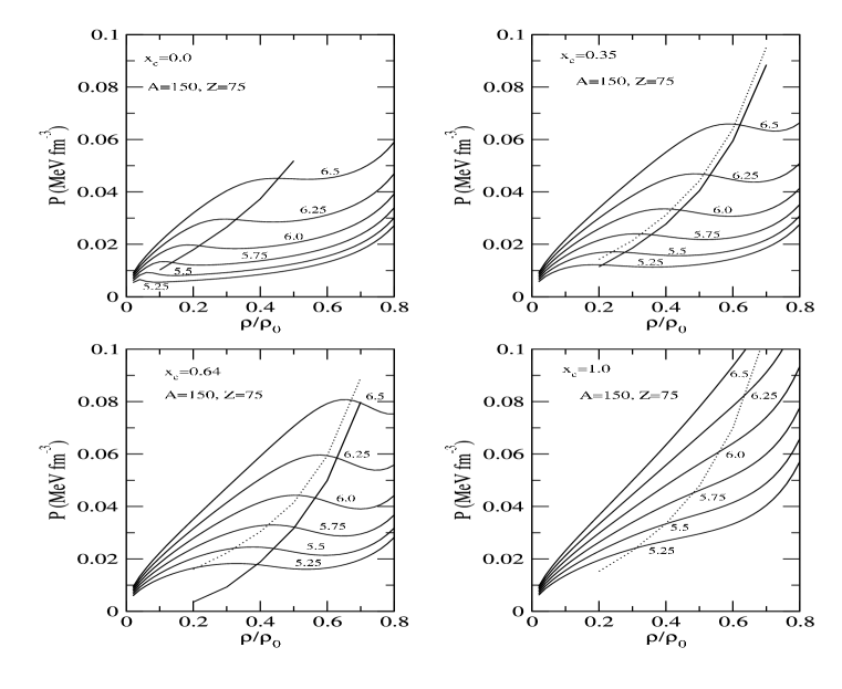
For a hypothetical nucleus of mass , atomic number and with no Coulomb force, we plot the functional relation between pressure and total density in the upper left part of Fig.1. A few comments about EoS in the model are in order.
The choice of a symmetric system was done to avoid mixing density and isospin effects, as we now explain. It is well known that phase transitions with two conserved charges (here: proton number and neutron number) can produce fractionation, i.e. different concentrations in the different phases. Then to spot the phase diagram of such a system the two densities have to be varied independentlyglendenning ; margueron ; ducoin . A projection of the two-dimensional equation of state on a specific axis, as for example the correlation at fixed , may be misleading, being continuous even in the occurrence of a discontinuous (first-order) transitionserot . This complication does not arise for symmetric matter, where fractionation disappears, the direction of phase separation follows the isoscalar density, and the whole information about the phase diagram is contained, as for one-fluid systems, in the equation of state. A first-order phase transition in this representation is unambiguously defined by the presence of a back-bending. Such behavior is very well known in the framework of the mean-field theory where it reflects the instability of homogeneous system with respect to phase separation. There, the appearence of a spinodal region reflects the inadequacy of the model. One needs to do a Maxwell or Gibbs construction before any correspondence with experiment can be established. It should be pointed out that the EoS in models like CTM are very different from those in the mean-field approximation, although a superficial look at Fig.1 would suggest this. There is a spinodal region in Fig.1 just as there is one in mean-field models, and in both cases they reflect phase separation. to see the effects of iso-spin in the model. The two EoS are quite similar. However, the backbending in CTM is an expected feature in the exact evaluation of the thermodynamics of a finite system which, at the thermodynamic limit, exhibits the discontinuity characteristic of a first-order phase transitiongross . The pressure decrease with density is physical, and it arises because of finite particle number imposed in the calculation. For earlier discussions on this see prl99 ; Das2 . In particular, in a simpler version of CTM it was explicitly demonstrated that the backbending disappears as the system grows and becomes a straight line with zero slope as expected in a first-order transitionChaudhuri2 . The height of the straight line, that is the value of the transition pressure for a given temperature, is given by the average pressure in the backbending regionChaudhuri2 ; noi .
Because of the preceeding discussion, we can conclude from Fig.1 that CTM presents a first-order transition between a dense, liquid-like phase and a dilute, gas-like one. The resulting phase diagram is reported in Fig.2, where the average pressure in the backbending region has been reported as a function of the temperature. The qualitative similarity with liquid-gas is apparent. It has been usual to limit the EoS in the in CTM to . The argument is that at higher densities the approximation of replacing the effect of the residual nuclear interaction between composites by just a constant excluded volume will begin to get worse. Here however both in Figs.1 and 2 the curves go beyond this.
We consider now bimodality in the value of as a function of where is the probability that the charge of the largest cluster in an event is . The significance of a bimodal distribution in a finite system as a signature of first-order transition has been extensively discussed in the literature pre ; noi ; binder . Here we do the calculation at a given density for different temperatures to locate the temperature where the two peaks of the bimodal distribution are nearly the same height. Having located the density and temperature we can then plot this as a point in the plane. At the same density we can also calculate the specific heat as a function of temperature and find the temperature where maximises. This gives us another point in the plane. Repeating the calculations for different densities we obtain two curves in the plane. A maximum in the value of is a generic signature of a phase transition with finite latent heat rounded by finite size effects. In the context of nuclear physics, it was taken as a possible signature of the transition associated to multifragmentation a long time ago Bondorf2 .
The remarkable thing is that without the Coulomb interaction the line representing bimodality and the maximum of coincide and fall in the backbending region. Both curves correspond to maxima of fluctuations: a peak in means maximal energy fluctuations, and fluctuations in the size of the largest cluster are maximum at the bimodality point. In a statistical ensemble where the freeze-out volume would be free to fluctuate under the effect of an external pressure, it is easy to show that the system would also present a bimodality in the volume distribution and a maximum in volume fluctuation at the pressure corresponding to the backbendingnoi ; raduta .
The coincidence of all these fluctuation signals agrees with the expectation that the fragmentation transition is very close to ordinary liquid-gas. Increasing the available volume at constant temperature, the system experiences a transition from configurations dominated by a single huge cluster at low excitation energy, to a highly fragmented pattern at high excitation energy. This transition can be classified as first-order in the sense that it would become discontinuous at the thermodynamic limit. In more technical terms, we can say that energy, particle density and are all order parameters of the observed transition. In a system as small as of course all observables are continuous, however the transition point can be uniquely determined by the location of the jump (for and ) or the fluctuation peak (for ) of the different order parameters.
This is shown by the phase diagram of Fig.2. The three different observables lead to a consistent estimation of the transition line.
The situation changes with Coulomb force. We introduce a strength parameter for the Coulomb force: =0 means no Coulomb and means the full Coulomb.
Figs. 1 and 2 report the results on the isotherms, fluctuation loci and phase diagram as the strength of the Coulomb force changes from through intermediate values to its full value .
Let us look at the EoS first. We can see that the inclusion of the Coulomb interaction results in a shift of the isotherms, with a gas-like branch appearing at higher density respect to the uncharged case, and a lower transition temperature for a given pressure. Moderately charged systems up to still show a phase diagram qualitatively similar to the uncharged case, but for the physical system the isotherms monotonously grow and the phase transition has disappeared. These features are in qualitative agreement with previous worksison ; raduta , as well as with the well-known expectation that the transition temperature should vanish approaching the drip-linesbonche .
The information given by the distribution of the largest fragment closely follows these thermodynamic findings. The bimodality line falls in the middle of the spinodal region for all values of , and bimodality disappears together with the phase transition in the fully charged case. Indeed the system is beyond the proton drip-line of the model, meaning that huge clusters close to the size of the source are unbound even at T=0.
The situation is different for the curve of maximum . This curve can be defined even for , where the system is fragmented at any temperature and no phase transition is observed. This shows that a peak in is a necessary but not sufficient condition for a first-order transitiongul99 . When the transition is present, Fig.2 shows that the observable leads to a definition of the phase diagram consistent with the isotherms and with the bimodality. However, we can see from Fig.1 that as the strength of the Coulomb force changes from through intermediate values to its full value, the splitting between the indicators of phase transitions progressively increases. Specifically, energy fluctuations peak at a density lower than the one one corresponding to the spinodal region in the charged system. The fluctuation energy peak is thus obtained within a pure phase.
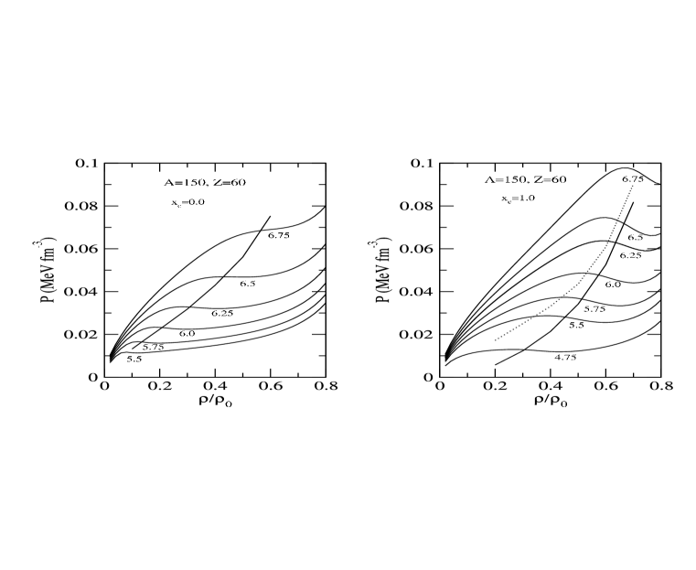
Of course experimentally we only see =1. theoretically. As discussed above, the disappearence of the transition for =1 is due to the fact that the considered system is beyond the proton drip-line. The more neutron rich system has the same size and the same Coulomb energy as our artificial with . This nucleus is not isospin symmetric, meaning that the correlation is not enough to trace the phase diagram of this system and a complete thermodynamic study would need the analysis of the whole two-dimensional equation of state.
However Fig.3 shows that isospin effects have a small influence in the correlation of CTM. This is at variance with mean-field models for infinite nuclear matterducoin ; serot . This is not so surprising recalling that in CTM the pressure is simply proportional to the total fragment multiplicitydas1 , and this latter is only slightly affected by the isospin. Thus the isotherms of the asymmetric system are very close to the isotherms of the corresponding symmetric system shown in Fig.1, once is chosen such as to have the same Coulomb energy as in the physical system. The same is true for the bimodality and signal, which are typical isoscalar observables strongly affected by Coulomb but not very sensitive to isospin. The preceeding discussion implies that the modification of the phase transition observed for in Figs.1,2 may be observed in a physically existing system like . This latter is close to the fragmention sources studied experimentally in refs.pichon ; bruno ; bonnet ; Neindre .
The splitting of the two fluctuation signals observed in Fig.3 suggests that the nature of the phase transition in charged systems may be different from that of uncharged ones. In particular in a transition with non-zero latent heat like liquid-gas the heat capacity should peak at the transition point, at variance with our results. This means that energy does not seem a good order parameter of the transition observed in CTM for charged nuclei. This last finding is very close to the study of ref.raduta . In that work it was shown that in the MMM fragmentation model in the isobar canonical ensemble the two bimodality peaks indicating the phase transition occur at very different Coulomb energies for heavily charged systems, but correspond to very similar excitation energies. If two phases are associated to the same energy, a mixing of the two does not induce any energy fluctuation, and the energy fluctuation at coexistence is the same as the energy fluctuation of the pure phases. Therefore we may expect that in the transition shown by CTM the two phases should correspond to similar excitation energies, or in other words that the latent heat of the transition should vanish with Coulomb.
To progress in the understanding of the observed phenomenon, we show in Fig.4 the distribution of the largest and second largest fragment at the bimodality point for the same system as in Fig.3. Not only the transition temperature is lowered by the inclusion of the Coulomb interaction as already observed, but the shape of the distribution is very different in the presence () or absence () of Coulomb. In the absence of Coulomb the two peaks are similar in shape and close to what is expected for the liquid-gas phase transition as depicted by the Lattice Gas Modelnpa : a liquid-like solution with a dominant cluster exhausting about 75% of the total mass, while the gas-like solution appearing at the same temperature consists of a much more fragmented configuration where the largest fragment is about 25% of the total size, and the second largest is of comparable size. The situation is completely different for the physical case where Coulomb is accounted for. In the presence of Coulomb the high-density solution corresponds essentially to the initial nucleus excited in its internal states. Such configurations give rise to what in nuclear physics is called an evaporation residue (recall secondary decay is not accounted for in CTM). The low-density solution is very different from the picture of a nuclear gas: the largest cluster is peaked at and the second largest has a very broad distribution ranging from to , and is close to the phenomenology expected for hot asymmetric fission.
V Summary
In this paper we have studied the effect of the Coulomb interaction on the fragmentation transition which is observed at finite temperature in the Canonical Thermodynamic Model. The typical behavior which is expected for a finite system counterpart of the liquid-gas phase transition is only observed if the Coulomb interaction is artificially switched off. The transition temperature decreases with increasing Coulomb energy as observed already in many other modelsdas1 ; ison ; raduta ; bonche . More interesting, the fragmentation pattern associated to the transition changes completely in the presence of Coulomb. In the spinodal region defined by the backbending of the isotherms the distribution of the largest fragment is bimodal. The two dominant fragmentation patterns defined by the two peaks at the bimodality point do not correspond to a liquid-gas phenomenology but are close to a transition from evaporation to asymmetric fission.
CTM was recently shown to produce results which are close to another very successful model of nuclear fragmentation, the Copenhagen SMMBotvina . Because of that, we think that the presented results are not specific to our model but should be characteristic of any model of fragmentation in statistical equilibrium.
The distribution of the largest fragment as a possible signature of a fragmentation transition is extensively studied experimentallypichon ; bruno ; bonnet ; Neindre in quasi-projectile fragmentation of Au+Au collisions. The comparison of CTM with experimental bimodality data will allow to progress on the interpretation of the transition observed in the data which is presently the object of intense debatelacroix ; trautmann ; aichelin ; npa . This will be the subject of a forthcoming paper.
VI Acknowledgement
This work is supported by the Natural Sciences and Engineering Research Council of Canada and by the National Science Foundation under Grant No PHY-0606007.
References
- (1) Ph. Chomaz, F. Gulminelli and V. Duflot, Phys. Rev. E 64, 046114, (2001); F. Gulminelli, Ph.Chomaz, Phys. Rev. C 71, 054607 (2005).
- (2) M. Pichon et al., Nucl. Phys. A 779, 267 (2006).
- (3) M. Bruno et al., Nucl. Phys. A 807, 48 (2008).
- (4) E.Bonnet, PhD Thesis, Université Paris XI, 2006, http://tel.archives-ouvertes.fr/tel-00121736.
- (5) O. Lopez et al., Phys. Rev. Lett. 95, 242701 (2005).
- (6) W. Trautmann, arXiv:nucl-ex/0705.0678.
- (7) A. Le Fèvre, J. Aichelin, Phys. Rev. Lett. 100, 042701 (2008).
- (8) F.Gulminelli, Nucl.Phys. A 791, 165 (2007).
- (9) C. B. Das, S. Das Gupta, W. G. Lynch, A. Z. Mekjian, and M. B. Tsang, Phys. Rep 406, 1, (2005)
- (10) N. Le Neindre et al., Nucl. Phys. A 795, 47 (2007).
- (11) M. D’Agostino et al., Nucl. Phys. A 650, 329 (1999).
- (12) G. Chaudhuri and S. Das Gupta, Phys. Rev. C75, 034603 (2007).
- (13) J. P. Bondorf, A. S. Botvina, A. S. Iljinov, I. N. Mishustin and K. Sneppen, Phys. Rep. 257, 133(1995).
- (14) B.Borderie, M.F.Rivet, Prog. Part. Nucl. Phys. (2008), and references therein.
- (15) R. Botet, M. Ploszajczak, Phys.Rev. E 62, 1825 (2000).
- (16) N. Bellaize et al., Nucl. Phys. A 709, 367 (2002).
- (17) B. Borderie, J. Phys. G. 28, R217 (2002); M. Rivet, et al., Nucl.Phys. A 749, 73 (2005).
- (18) N.K.Glendenning, Phys. Rep. 342, 393 (2001).
- (19) J.Margueron, Ph. Chomaz, Phys. Rev. C 67, 041602 (2003).
- (20) C.Ducoin, Ph.Chomaz, F. Gulminelli, Nucl.Phys.A 771, 68 (2006).
- (21) H.Muller and B.Serot, Phys. Rev. C 52, 2072 (1995).
- (22) D. H. E. Gross, ”Microcanonical thermodynamics: phase transitions in finite systems”, Lecture notes in Physics vol. 66, World Scientific (2001).
- (23) Ph.Chomaz, F.Gulminelli, Phys. Rev. Lett. 82, 1402 (1999).
- (24) C. B. Das, S. Das Gupta and A. Z. Mekjian, Phys. Rev. C 67, 064607 (2003).
- (25) G. Chaudhuri and S. Das Gupta, Phys. Rev C 76, 014619 (2007).
- (26) Ph.Chomaz and F.Gulminelli, in ’Dynamics and Thermodynamics of systems with long range interactions’, Lecture Notes in Physics vol.602, Springer (2002).
- (27) K. Binder and D. P. Landau, Phys. Rev. B 30, 1477 (1984).
- (28) J. Bondorf, R. Donangelo, I. M. Mishustin and H. Schulz, Nucl. Phys. A444(1985)460
- (29) M.J.Ison, C.O.Dorso, Phys.Rev. C 69, 027001 (2004).
- (30) F.Gulminelli, Ph.Chomaz, A.H.Raduta, A.R.Raduta, Phys.Rev.Lett. 91, 202701 (2003).
- (31) P. Bonche et al., Nucl. Phys. A 427, 278 (1984).
- (32) Ph. Chomaz et F. Gulminelli, Nucl. Phys. A 647,153 (1999).
- (33) A. Botvina, G. Chaudhuri, S. Das Gupta and I. Mishustin, arXiv:0805.3514v1[nucl-th].