Deformed quasiparticle-random-phase approximation for neutron-rich nuclei using the Skyrme energy density functional

Abstract

We develop a new framework of the deformed quasiparticle-random-phase approximation (QRPA) where the Skyrme density functional and the density-dependent pairing functional are consistently treated. Numerical applications are carried out for the isovector dipole and the isoscalar quadrupole modes in the spherical ²⁰O and in the deformed ²⁶Ne nuclei, and the effect of the momentum dependent terms of the Skyrme effective interaction for the energy-weighted sum rule is discussed. As a further application, we present for the first time the moments of inertia of ³⁴Mg and ³⁶Mg using the Thouless-Valatin procedure based on the self-consistent deformed QRPA, and show the applicability of our new calculation scheme not only for the vibrational modes but also for the rotational modes in neutron-rich nuclei.

I Introduction

Exploring nuclei far from the stability line is one of the most actively studied fields in nuclear physics. The exotic nuclei have revealed many features of atomic nuclei that are quite different from stable nuclei. Examples are the emergence of the neutron halo tan85 and the skin suz95 structures, the soft dipole excitations sac93 , the modifications of some magic numbers iwa00 ; gui84 and the appearance of new magic numbers instead oza00 , the onset of new regions of deformation mot95 . These new features are strongly connected with the presence of the loosely bound neutrons and the coupling with the positive energy continuum states. Under the new environment, the nuclear many-body correlations such as the pairing and the deformation could have also unique features in exotic nuclei dob84 ; dob96 ; ben99 ; ben00b ; mis97 ; ham04a ; yos05a ; ham04 ; ham05 .

For describing multipole responses in exotic nuclei in the region of medium-heavy systems, there have been many attempts employing the particle-hole random phase approximation (RPA) ham96 ; ham99 ; shl03 or the quasiparticle-RPA (QRPA) mat01 ; mat05 ; miz07 ; hag01 ; kha02 ; yam04 ; ter05 ; ter06 ; vre01 ; paa03 ; paa04 ; paa05 ; cao05 ; gia03 ; sar04 ; per05 on top of the self-consistent Hartree-Fock (HF) or Hartree-Fock-Bogoliubov (HFB) mean fields. (See Refs. ben03 ; vre05 ; paa07 for extensive lists of references concerning the self-consistent (Q)RPA and mean-field calculations.) These studies are largely restricted to spherical systems. Recently, low-lying RPA modes in deformed neutron-rich nuclei have been investigated by several groups yos05 ; nak05 ; ina06 ; sar98 ; mor06 ; urk01 ; hag04a ; pen07 . These calculations, however, do not take into account the pairing correlations, or rely on the BCS approximation for pairing, which is inappropriate for describing the pairing correlations in drip line nuclei due to the unphysical nucleon gas problem dob84 .

In order to discuss simultaneously effects of nuclear deformation and pairing correlations including the unbound quasiparticle states, we have developed in Ref. yos06 a calculation scheme that carried out the deformed QRPA calculation based on the coordinate-space HFB formalism. The residual interaction in the particle-hole (p-h) channel was a simplified Skyrme interaction neglecting the momentum dependence ber91 while a deformed Woods-Saxon potential was employed for the mean field. In Ref. yos08 , one step further was accomplished by using a self-consistent Skyrme-HFB deformed mean field while the p-h residual interaction corresponding to the same Skyrme force was approximated by its Landau-Migdal (LM) form bac75 ; gia81 . However, the resulting energy-weighted sum rule (EWSR) for the isovector dipole response was not fulfilled very accurately.

A full consistency between the QRPA and HFB calculations is required for a quantitative description of the multipole strengths in exotic nuclei. This means that the same effective interaction or the same energy density functional is used for both calculations. We note that fully consistent HFB+QRPA calculations with the Gogny effective interaction for deformed nuclei are now available per08 , but the use of a harmonic oscillator basis is a drawback for describing the unique spatial structure of quasiparticle wave functions near the Fermi level in neutron drip-line nuclei.

We therefore develop in this article a new method for solving the Skyrme-HFB-QRPA problem in deformed systems while keeping the full velocity dependence of the p-h residual interaction. The Skyrme-HFB mean field is calculated in the coordinate-space representation. Numerical calculations are performed in order to investigate the effects of the explicit treatment of the momentum-dependent terms of the effective interaction on the EWSR of multipole responses and on the moments of inertia of deformed neutron-rich nuclei. The decoupling between the spurious mode of translation and intrinsic excitations is reasonably obtained in these consistent calculations.

The article is organized as follows: In Sec. II, the method is explained. In Sec. III, we perform the numerical calculations and investigate properties of the isovector/isoscalar dipole and the isoscalar quadrupole modes in ²⁰O, the isovector/isoscalar dipole modes in ²⁶Ne, and the moments of inertia of ³⁴Mg and ³⁶Mg as well as the isoscalar quadrupole mode. Sec. IV contains the conclusions. We summarize in the Appendix the main formulas relevant to the Skyrme energy density functional to show clearly what are the terms that are included in our approach.

II Method

In the present section, we explain our method of the deformed QRPA based on the Skyrme density functional. We solve the HFB equations dob84 ; bul80

$$\begin{pmatrix}h^{q}(\bm{r},\sigma)-\lambda^{q}&\tilde{h}^{q}(\bm{r},\sigma)\\ \tilde{h}^{q}(\bm{r},\sigma)&-(h^{q}(\bm{r},\sigma)-\lambda^{q})\end{pmatrix}\begin{pmatrix}\varphi^{q}_{1,\alpha}(\bm{r},\sigma)\\ \varphi^{q}_{2,\alpha}(\bm{r},\sigma)\end{pmatrix}$$

$$=E_{\alpha}\begin{pmatrix}\varphi^{q}_{1,\alpha}(\bm{r},\sigma)\\ \varphi^{q}_{2,\alpha}(\bm{r},\sigma)\end{pmatrix}$$ (1)

in coordinate space using cylindrical coordinates $\bm{r}=(\rho,z,\phi)$. We assume axial and reflection symmetries. Here, $q=\nu$ (neutron) or $\pi$ (proton). For the mean-field Hamiltonian $h$, we employ the SkM* interaction bar82 in the present numerical applications. Details for expressing the densities and currents in the cylindrical coordinate representation can be found in Refs. ter03 ; sto05 . The pairing field is treated by using the density-dependent contact interaction cha76 ,

$$v_{pair}(\bm{r},\bm{r}^{\prime})=\dfrac{1-P_{\sigma}}{2}\left[t_{0}^{\prime}+\dfrac{t_{3}^{\prime}}{6}\varrho_{0}^{\gamma}(\bm{r})\right]\delta(\bm{r}-\bm{r}^{\prime}).$$ (2)

where $\varrho_{0}(\bm{r})$ denotes the isoscalar density and $P_{\sigma}$ the spin exchange operator. Assuming time-reversal symmetry and reflection symmetry with respect to the $x-y$ plane, we have only to solve for positive $\Omega$ and positive $z$. We use the lattice mesh size $\Delta\rho=\Delta z=0.6$ fm and a box boundary condition at ($\rho_{\mathrm{max}}=9.9$ fm, $z_{\mathrm{max}}=9.6$ fm) for ²⁰O and ²⁶Ne, and ($\rho_{\mathrm{max}}=9.9$ fm, $z_{\mathrm{max}}=12$ fm) for Mg isotopes. The quasiparticle energy cutoff is chosen at $E_{\mathrm{qp,cut}}=60$ MeV and the quasiparticle states up to $\Omega^{\pi}=15/2^{\pm}$ are included (for ²⁶Ne, we include the quasiparticle states up to $\Omega^{\pi}=13/2^{\pm}$ in order to compare with the results of Ref. yos08 ). Our calculation scheme for solving the HFB equations is quite similar to Ref. oba08 , whereas the reflection symmetry was not imposed in Ref. oba08 .

Using the quasiparticle basis obtained as the self-consistent solution of the HFB equations (1), we solve the QRPA equation in the matrix formulation row70

$$\sum_{\gamma\delta}\begin{pmatrix}A_{\alpha\beta\gamma\delta}&B_{\alpha\beta\gamma\delta}\\ B_{\alpha\beta\gamma\delta}&A_{\alpha\beta\gamma\delta}\end{pmatrix}\begin{pmatrix}X_{\gamma\delta}^{\lambda}\\ Y_{\gamma\delta}^{\lambda}\end{pmatrix}=\hbar\omega_{\lambda}\begin{pmatrix}1&0\\ 0&-1\end{pmatrix}\begin{pmatrix}X_{\alpha\beta}^{\lambda}\\ Y_{\alpha\beta}^{\lambda}\end{pmatrix}.$$ (3)

The residual interaction in the particle-hole (p-h) channel appearing in the QRPA matrices $A$ and $B$ is derived from the Skyrme density functional,

$$v_{ph}(\bm{r},\bm{r}^{\prime})=\dfrac{\delta^{2}\mathcal{E}_{\mathrm{Sky}}}{\delta\varrho(\bm{r}^{\prime})\delta\varrho(\bm{r})},$$ (4)

where we neglect the spin-orbit interaction term $C_{t}^{\nabla J}$ in Eq. (18) as well as the Coulomb interaction to reduce the computing time. We also drop the so-called $``{J}^{2}"$ term $C_{t}^{T}$ in both the HFB and QRPA calculations. Thus, the residual interaction reads

$$v_{ph}(\bm{r},\bm{r}^{\prime}) =(a_{0}+a_{0}^{\prime}\tau\cdot\tau^{\prime}+(b_{0}+b_{0}^{\prime}\tau\cdot\tau^{\prime})\sigma\cdot\sigma^{\prime})\delta(\bm{r}-\bm{r}^{\prime})$$

$$+(a_{1}+a_{1}^{\prime}\tau\cdot\tau^{\prime}+(b_{1}+b_{1}^{\prime}\tau\cdot\tau^{\prime})\sigma\cdot\sigma^{\prime})$$

$$\times(\bm{k}^{\dagger 2}\delta(\bm{r}-\bm{r}^{\prime})+\delta(\bm{r}-\bm{r}^{\prime})\bm{k}^{2})$$

$$+(a_{2}+a_{2}^{\prime}\tau\cdot\tau^{\prime}+(b_{2}+b_{2}^{\prime}\tau\cdot\tau^{\prime})\sigma\cdot\sigma^{\prime})$$

$$\times(\bm{k}^{\dagger}\cdot\delta(\bm{r}-\bm{r}^{\prime})\bm{k}),$$ (5)

where $\bm{k}=(\overrightarrow{\nabla}-\overrightarrow{\nabla}^{\prime})/2i$ and $\bm{k}^{\dagger}=-(\overleftarrow{\nabla}-\overleftarrow{\nabla}^{\prime})/2i$. The coefficients in Eq. (5) are given in Ref. ter05 (For simplicity, the coefficients $a_{0},a_{0}^{\prime},b_{0}$ and $b_{0}^{\prime}$ here include the density dependent terms and rearrangement terms of $a_{3}-f_{3}$ in Ref. ter05 ). We do not include the pairing rearrangement terms coming from the second derivative of the pairing functional $\mathcal{E}_{\mathrm{pair}}$ with respect to the normal density $\varrho$.

On the other hand, the residual interaction in the particle-particle (p-p) channel is derived from the pairing functional constructed with the density-dependent contact interaction (2),

$$v_{pp}(\bm{r},\bm{r}^{\prime})=\dfrac{\delta^{2}\mathcal{E}_{\mathrm{pair}}}{\delta\tilde{\varrho}(\bm{r}^{\prime})\delta\tilde{\varrho}(\bm{r})}.$$ (6)

This altogether coincides with Eq. (2).

Because the full self-consistency between the static mean-field calculation and the dynamical calculation is broken by the above neglected terms, we renormalize the residual interaction in the p-h channel by an overall factor $f_{ph}$ to get the spurious $K^{\pi}=0^{-}$ and $1^{-}$ modes (representing the center-of-mass motion), and $K^{\pi}=1^{+}$ mode (representing the rotational motion in deformed nuclei) at zero energy ($v_{ph}\rightarrow f_{ph}\cdot v_{ph}$). We cut the two-quasiparticle (2qp) space at $E_{\alpha}+E_{\beta}\leq 60$ MeV due to the excessively demanding computer memory size and computing time for the model space consistent with that adopted in the HFB calculation. Accordingly, we need another factor $f_{pp}$ for the p-p channel. We determine this factor such that the spurious $K^{\pi}=0^{+}$ mode associated with the particle number fluctuation (representing the pairing rotational mode) appears at zero energy ($v_{pp}\rightarrow f_{pp}\cdot v_{pp}$).

III Results and Discussion

III.1 ²⁰O

The application of our new calculation scheme is presented at first for a spherical system. In Ref. miz07 , detailed properties of ²⁰O were investigated using the continuum QRPA based on the Skyrme density functional. In the present subsection, we show our results for the isovector dipole and isoscalar quadrupole modes in ²⁰O following the discussions in Ref. miz07 . In the HFB calculations, the pairing strengths $t_{0}^{\prime}=-280$ MeV$\cdot$fm³ and $t_{3}^{\prime}=-18.75t_{0}^{\prime}$ with $\gamma=1$ are employed as in Ref. miz07 . With the choice $\gamma=1$ in the pairing interaction, the pairing rearrangement terms vanish in the residual interaction.

Because we use a larger mesh size and a smaller box, the obtained solution is not exactly the same as in Ref. miz07 ; the calculated total binding energy is 157.7 MeV and the average neutron pairing gap is $\langle\Delta\rangle_{\nu}=1.92$ MeV. There are also differences in the QRPA calculations between the two calculations: the boundary conditions, the 2qp cutoff energy and the treatment of the spin-dependent interactions ($\sigma\cdot\sigma^{\prime}$ terms in Eq. (5)). In the present calculation, the transition spin density is treated exactly.

Figure 1: The 2qp cutoff-energy dependence of the $B(E2\uparrow)$ values (upper panel) and excitation energies $E(2^{+})$ (lower panel) for the first excited $2^{+}$ state in ²⁰O.

In Fig. 1 we show the 2qp cutoff energy dependence of the excitation energies and electric quadrupole transition strengths of the first excited state. In this figure, we show the excitation energies of the $K^{\pi}=0^{+},1^{+}$ and $2^{+}$ states. If the spherical symmetry is preserved perfectly, these energies should be degenerate. In the actual calculation, however, the spherical symmetry is broken due to the finite mesh size. Therefore, we can consider this difference ($\sim 150$ keV) as the numerical error caused by the discretization of the coordinates. The transition strength $B(E2\uparrow)$ is a sum of the intrinsic transition strengths to the $K^{\pi}=0^{+},\pm 1^{+}$ and $\pm 2^{+}$ states. Around the cutoff energy at 50 MeV, one can see that both $E(2^{+})$ and $B(E2\uparrow)$ converge enough.

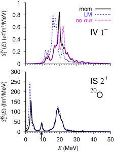
Figure 2: Response functions for the isovector dipole (upper panel) and the isoscalar quadrupole (lower panel) operators in ²⁰O. The dotted and solid lines correspond to the Landau-Migdal approximation (LM) and the full calculation taken into account the momentum dependence explicitly (mom). The dashed line denotes the calculation without the $\sigma\cdot\sigma^{\prime}$ interaction while keeping the momentum dependence explicitly. The transition strengths are smeared by a Lorentzian function with a width of $\Gamma=1$ MeV. The arrow indicates the neutron emission threshold $E_{\mathrm{th}}=9.19$ MeV.

We show in Fig. 2 the response functions for the isovector (IV) dipole and the isoscalar (IS) quadrupole operators

$$\hat{F}_{1K}^{\mathrm{IV}} =e\dfrac{N}{A}\sum_{i}^{Z}r_{i}Y_{1K}(\hat{r}_{i})-e\dfrac{Z}{A}\sum_{i}^{N}r_{i}Y_{1K}(\hat{r}_{i}),$$ (7a)

$$\hat{F}_{2K}^{\mathrm{IS}} =\sum_{i}^{A}r^{2}_{i}Y_{2K}(\hat{r}_{i}),$$ (7b)

and the corresponding response functions defined as

$$S_{\lambda}^{\tau}(E)=\sum_{i}\sum_{K}\dfrac{\Gamma/2}{\pi}\dfrac{|\langle i|\hat{F}_{\lambda K}^{\tau}|0\rangle|^{2}}{(E-\hbar\omega_{i})^{2}+\Gamma^{2}/4}.$$ (8)

In this figure, we also show the response functions obtained by using the LM approximation. This approximation treats only approximately the momentum dependence of the Skyrme p-h residual interaction. The resulting contact force is defined by the density-dependent Landau parameters $F_{0},F_{0}^{\prime},G_{0}$ and $G_{0}^{\prime}$, which are determined by the parameters of the Skyrme effective interaction gia81 . The renormalization factors for the full QRPA calculation are $f_{ph}=1.095$ and $f_{pp}=1.180$, while $f_{ph}=0.815$ in the LM approximation.

For the IV dipole mode, the location of the giant resonance is quite different between the calculation in the LM approximation and that taking fully into account the momentum dependence. The peak position is shifted up in the latter case. In Ref. miz07 , the same tendency was obtained. However, the shape of the giant resonance is different between the two calculations. This difference comes from the $\sigma\cdot\sigma^{\prime}$ terms of the p-h interaction which were omitted in Ref. miz07 . Indeed, if we drop these terms in our calculation we obtain a two-peak structure (see Fig. 2) which is consistent with the result of Ref. miz07 .

For the IS quadrupole mode, we can see a prominent peak at $2-3$ MeV, as well as the giant resonance at around 20 MeV. The low-lying state is sensitive to the momentum-dependent components of the force while the position of the giant resonance remains the same. In both calculations we obtain a small peak at 9 MeV just above the threshold, but the transition strength and the excitation energy are not affected. This result is consistent with Ref. miz07 .

Figure 3: Energy weighted sum of the IV dipole and IS quadrupole strength functions. The solid and dotted lines represent the calculation taking into account the momentum dependence explicitly (mom) and in the Landau-Migdal approximation (LM), respectively. The horizontal lines show the classical Thomas-Reiche-Kuhn (TRK), and the RPA sum rule values for the isovector case including the enhancement factor, $m_{1}=m_{1}^{\mathrm{cl}}(1+\kappa)$ ($\kappa=0.32$ in ²⁰O with the SkM* interaction ). For the isoscalar case, the EWSR corresponds to the classical sum-rule value.

Figure 3 shows the partial sum of the energy weighted strength defined as

$$W(E_{x})=\sum_{\hbar\omega_{i}<E_{x}}\hbar\omega_{i}|\langle i|\hat{F}_{\lambda}^{\tau}|0\rangle|^{2}.$$ (9)

For the IV dipole mode, the calculated sum up to 60 MeV reaches 99.5% of the EWSR value including the enhancement factor, $m_{1}=m_{1}^{\mathrm{cl}}(1+\kappa)$ ter06 where $\kappa=0.32$, whereas the calculation in the LM approximation underestimates by 13% the EWSR value. For the IS quadrupole mode, the calculated sum satisfies 98.9% of the EWSR value, which is comparable to the values obtained in Ref. miz07 . The calculation in the LM approximation overestimates by 9.3% the EWSR value. This accuracy is as same as in Ref. miz07 .

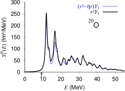
Figure 4: Response functions for the IS dipole operators Eqs. (10) and (11) in ²⁰O.

Next, we discuss the decoupling of the spurious state from the physical states. The IS dipole compression mode is sensitive to the admixture of the center-of-mass motion ham02 because the response function to the IS dipole operator

$$\hat{F}_{1K}^{\mathrm{IS}}=\sum_{i}^{A}r^{3}_{i}Y_{1K}(\hat{r}_{i})$$ (10)

contains the strengths of both the spurious mode and physical intrinsic excitations. In order to see how much the spurious component mixes to the physical states, we compare the response function to the operator Eq. (10) with that to the corrected operator har81 ; gia81b

$$\hat{F}_{1K}^{\mathrm{IS(cor)}}=\sum_{i}^{A}(r^{3}_{i}-\eta r_{i})Y_{1K}(\hat{r}_{i}),$$ (11)

where $\eta=\frac{3}{5}\langle r^{2}\rangle$. If the spurious component is completely removed from the intrinsic excitations, the calculated response functions to the operators Eqs. (10) and (11) should coincide with each other.

Figure 4 shows the response functions to the IS dipole operators Eqs. (10) and (11). At around 17 MeV, we can see a slight difference between the two responses. In Ref. ter05 , the admixture of the spurious component was investigated in detail. Accurate results could be obtained by using a very large cutoff energy of 140 MeV in the 1qp spectrum included in the fully self-consistent QRPA calculations. In the present work, the 2qp space is much smaller than in Ref. ter05 and some of the residual interactions are not included. Though there is some room for further improvements, the results obtained here are rather satisfactory.

III.2 ²⁶Ne

In Ref. yos08 , we have studied the properties of the low-lying isovector resonance in deformed ²⁶Ne using the LM approximation. Although the strength function observed at RIKEN gib07 could be well reproduced, the EWSR was not satisfied very accurately. In the present subsection, we present the QRPA results where the momentum dependence of $v_{ph}$ is fully included and we show how the EWSR is fulfilled with the new method. The parameters in the HFB calculation are the same as in Ref. yos08 , the difference being only in the treatment of the momentum dependent terms of interaction in the QRPA calculation.

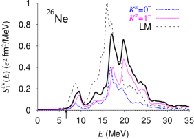
Figure 5: Response functions for the isovector dipole operator in ²⁶Ne. The dotted, dashed and solid lines correspond to the $K^{\pi}=0^{-}$, $K^{\pi}=1^{-}$ and total responses, respectively. The thin dotted line represents the response in the LM approximation. For the $K^{\pi}=1^{-}$ response, the transition strengths for the $K^{\pi}=\pm 1^{-}$ states are summed up. The arrow indicates the neutron emission threshold $E_{\mathrm{th}}=6.58$ MeV.

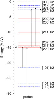
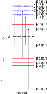
Figure 6: Two-quasiparticle (particle-hole) excitations generating the $K^{\pi}=0^{-}$ state at 8.68 MeV in ²⁶Ne. The single-particle levels are labeled with the asymptotic quantum numbers $[Nn_{3}\Lambda]\Omega$. The solid and dotted lines stand for the positive and negative parities, respectively. The chemical potential $\lambda$ is indicated by the two-dotted line.

Table 1: QRPA amplitudes for the $K^{\pi}=0^{-}$ state at 8.68 MeV in ²⁶Ne. This mode has the isovector strength $B(Q^{\mathrm{IV}}1)=8.72\times 10^{-2}e^{2}$fm², and the sum of backward-going amplitudes $\sum|Y_{\alpha\beta}|^{2}=5.24\times 10^{-3}$. Only components with $X_{\alpha\beta}^{2}-Y_{\alpha\beta}^{2}>0.001$ are listed. In the rows (h) and (i), the label $\nu 1/2^{-}$ denotes a non-resonant discretized continuum state of neutron $\Omega^{\pi}=1/2^{-}$ level.

			$E_{\alpha}+E_{\beta}$		$Q_{10,\alpha\beta}$
	$\alpha$	$\beta$	(MeV)	$X_{\alpha\beta}^{2}-Y_{\alpha\beta}^{2}$	($e\cdot$ fm)
(a)	$\nu[310]1/2$	$\nu[211]1/2$	8.15	0.747	$-0.309$
(b)	$\nu[330]1/2$	$\nu[220]1/2$	11.4	0.034	$-0.397$
(c)	$\nu[321]3/2$	$\nu[211]3/2$	11.3	0.023	0.338
(d)	$\nu[312]5/2$	$\nu[202]5/2$	11.2	0.011	$-0.239$
(e)	$\nu[330]1/2$	$\nu[211]1/2$	6.54	0.015	$-0.118$
(f)	$\nu[200]1/2$	$\nu[101]1/2$	14.0	0.004	$-0.241$
(g)	$\nu[301]1/2$	$\nu[211]1/2$	9.32	0.003	$-0.117$
(h)	$\nu 1/2^{-}$	$\nu[211]1/2$	12.6	0.008	$-0.068$
(i)	$\nu 1/2^{-}$	$\nu[211]1/2$	13.7	0.004	$-0.077$
(j)	$\pi[220]1/2$	$\pi[101]1/2$	7.96	0.125	0.0085
(k)	$\pi[220]1/2$	$\pi[110]1/2$	14.1	0.014	$-0.346$
(l)	$\pi[330]1/2$	$\pi[220]1/2$	13.4	0.013	$-0.329$
(m)	$\pi[321]3/2$	$\pi[211]3/2$	14.0	0.004	$-0.372$

Figure 7: Same as Fig. 3 but for ²⁶Ne.

We show in Fig. 5 the response functions for the isovector dipole mode. The renormalization factors for the QRPA calculation are $f_{ph}=1.093$ and $f_{pp}=1.225$, while $f_{ph}=0.919$ in the LM approximation. Compared to the response functions obtained by using the LM approximation, the excitation energies of both the low-lying and giant resonances are slightly shifted up while the overall structure remains similar. We can clearly see the resonance structure below 10 MeV as experimentally observed gib07 . The resonance is governed by the $K^{\pi}=0^{-}$ state at 8.7 MeV and the $K^{\pi}=1^{-}$ states at 9.1 MeV and 9.6 MeV. The microscopic structure of the $K^{\pi}=0^{-}$ state is given in Fig. 6 and Table 1. Here, the single-particle states are obtained by rediagonalizing the self-consistent single-particle Hamiltonian $h$ of Eq. (1). As in the case of the LM approximation, this $K^{\pi}=0^{-}$ state contains mainly the neutron 1p-1h configuration $(2s_{1/2})^{-1}(2p_{3/2})$, whose squared amplitude is 0.75. The $K^{\pi}=1^{-}$ state at 9.1 MeV has also the same main component, with a weight of 0.83. The state at 9.6 MeV is mainly generated by the $(2s_{1/2})^{-1}(2p_{1/2})$ excitation with a weight of 0.90. A difference between the results of the LM approximation and the present results is that the transition strength to the $K^{\pi}=1^{-}$ state at 9.6 MeV (0.08$e^{2}$fm²) is larger than that to the state at 9.1 MeV (0.04$e^{2}$fm²).

Figure 7 shows the energy weighted sum of the isovector dipole strength function together with the sum rule values represented by the horizontal lines. The energy-weighted sum up to 60 MeV overestimates by only 1.6% the EWSR value including the enhancement factor $\kappa=0.32$. In the calculation with the LM approximation, the energy-weighted sum is underestimated by about 10% yos08 . This suggests that treating the momentum dependence of the Skyrme force explicitly in the QRPA calculation is crucial for satisfying the EWSR in the deformed systems as in the spherical systems miz07 . Because of the severe cutoff in the 2qp excitation energy, we cannot describe properly the energy region higher than the giant resonance. It would be interesting to see if calculations in a larger 2qp space including the residual spin-orbit and the Coulomb interactions can improve the overshooting of the EWSR value.

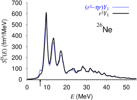
Figure 8: Same as Fig. 4 but for ²⁶Ne.

Next, we discuss the IS dipole response. The corrected IS dipole operator Eq. (11) with $\eta=\frac{3}{5}\langle r^{2}\rangle$ is valid only for the spherical systems. We can extend it for the deformed systems by following the discussion in Appendix of Ref. gia81b . One obtains the correction factor $\eta$ for the deformed systems

$$\eta=\begin{cases}3\langle z^{2}\rangle+\langle\rho^{2}\rangle&(K=0)\\ \langle z^{2}\rangle+2\langle\rho^{2}\rangle&(K=\pm 1).\end{cases}$$ (12)

These correction factors coincide with $\eta=\frac{3}{5}\langle r^{2}\rangle$ in the spherical limit.

In Fig. 8, we show the response functions to the IS dipole operators with/without the correction. For the lowest state at 6.5 MeV, we can see a difference between the two calculations. However, the overall structures are not very different. We can consider that the spurious component is well removed from the pygmy resonance and the giant resonance.

III.3 ²⁴Mg

We show in Fig. 9 the response functions for the IS quadrupole transition in ²⁴Mg. We employ the same effective interactions for the HFB+QRPA calculation as in the ²⁰O nucleus. The renormalization factor is $f_{ph}=1.164$. The giant resonance appears at around 15 – 25 MeV. Since the ground state is prolately deformed in our calculation ($\beta_{2}=0.4$), we can see a clear $K$-splitting. Below 5 MeV, we can see a prominent peak for the $K^{\pi}=2^{+}$ excitation. These are consistent with the fully self-consistent deformed QRPA calculation using the Gogny force per08 .

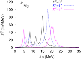
Figure 9: Response functions for the IS quadrupole transition in ²⁴Mg for the $K^{\pi}=0^{+},1^{+}$ and $2^{+}$ excitations represented by the solid, dotted and dashed lines, respectively.

Figure 10: Excitation energy spectrum obtained by the QRPA calculation and the available experimental data nds24 .

In Fig. 10, we show the low-lying excitation spectrum. Here excitation energies are evaluated by EG

$$E(I,K)=\hbar\omega_{\mathrm{RPA}}+\frac{\hbar^{2}}{2\mathcal{J}_{\mathrm{TV}}}(I(I+1)-K^{2}),$$ (13)

in terms of the vibrational frequencies, $\omega_{\mathrm{RPA}}$, and the Thouless-Valatin moment of inertia tho62 , $\mathcal{J}_{\mathrm{TV}}$, calculated microscopically by the QRPA. The calculated moment of inertia is large compared to the experimental rotational band. This is because the present pairing interaction leads to vanishing neutron and proton pairing gaps. Furthermore, due to the absence of the coupling mechanism between the $\beta$ vibration and the pairing vibration, the excited $K^{\pi}=0^{+}$ mode cannot acquire a substantial collectivity and the excitation energy remains large. The $\gamma$ vibrational mode reasonably reproduces the experiment. This $K^{\pi}=2^{+}$ state is mainly generated by the neutron and proton p-h excitations $[211]3/2\to[211]1/2$. Their contributions are 42% and 56%, respectively and the total transition strength is exhausted about 55% by the two p-h excitations. The rest of the transition strength comes from the coupling to the giant resonance.

III.4 ³⁴Mg and ³⁶Mg

Table 2: Ground state properties of ³⁴Mg and ³⁶Mg obtained by the deformed HFB calculation with the SkM* interaction and the mixed-type pairing interaction. Chemical potentials, deformations, average pairing gaps, root-mean-square radii for neutrons and protons, and the total binding energies are listed.

	34Mg	36Mg
$\lambda_{\nu}$ (MeV)	$-4.16$	$-3.24$
$\lambda_{\pi}$ (MeV)	$-19.8$	$-20.1$
$\beta_{2}^{\nu}$	0.35	0.31
$\beta_{2}^{\pi}$	0.41	0.39
$\langle\Delta\rangle_{\nu}$ (MeV)	1.71	1.71
$\langle\Delta\rangle_{\pi}$ (MeV)	0.0	0.0
$\sqrt{\langle r^{2}\rangle_{\nu}}$ (fm)	3.51	3.59
$\sqrt{\langle r^{2}\rangle_{\pi}}$ (fm)	3.16	3.18
$E_{\mathrm{total}}$ (MeV)	263.3	269.9

In Ref. yos08b , the properties of the low-lying $K^{\pi}=0^{+}$ mode in ³⁴Mg have been studied and the moments of inertia were calculated using the Thouless-Valatin method. In the present subsection, effects of the momentum dependent components of the Skyrme interaction on the isoscalar quadrupole strengths and the moments of inertia are discussed.

In the HFB calculations, the pairing strength parameter is determined so as to reproduce the experimental pairing gap of ³⁴Mg ($\Delta_{\mathrm{exp}}=1.7$ MeV) obtained by the three-point formula sat98 . In Table 2, the ground state properties of ^34,36Mg are summarized. The strength $t_{0}^{\prime}=-295$MeV$\cdot$fm³ for the mixed-type interaction with $\gamma=1$ leads to the pairing gaps $\langle\Delta_{\nu}\rangle=1.71$ MeV in ³⁴Mg and ³⁶Mg. We obtain for the proton intrinsic quadrupole moments $Q_{0}$ the values 62.2$e\cdot$fm² and 60.1$e\cdot$fm² in ³⁴Mg and ³⁶Mg, respectively. The reduced transition probabilities RS are then $B(E2;0^{+}\to 2_{1}^{+})=5/16\pi\cdot Q_{0}^{2}=385e^{2}\cdot$fm⁴ and 359 $e^{2}\cdot$fm⁴ in ³⁴Mg and ³⁶Mg. In ³⁴Mg, the neutron occupation probability of the [202]3/2 level coming up from the $1d_{3/2}$ orbit is 0.28, while that of the [321]3/2 level coming down from the $1f_{7/2}$ orbit is 0.67. This approximately corresponds to the $(1f_{7/2})^{4}(1d_{5/2})^{-2}$ configuration in the spherical shell model language. In ³⁶Mg, the occupation probability of the $\nu[202]3/2$ level becomes 0.64. These probabilities are consistent with the shell model results uts99 .

In the QRPA calculations of ³⁴Mg and ³⁶Mg, we cut the 2qp space at 60 MeV as in the previous subsections. We have checked that the transition strength to the excited $0^{+}$ state and its excitation energy converge at 50 MeV cutoff. In the present case, the dimension of the QRPA matrix (3) for the $K^{\pi}=0^{+}$ channel in ³⁶Mg is about 15,000, the memory size is 20.8 GB, and the CPU time is about 154,000s per iteration for determining the renormalization factor $f_{pp}$ using the SX-8 supercomputer at the RCNP.

Figure 11: Response functions for the IS quadrupole operator in ³⁴Mg (upper panel) and ³⁶Mg (lower panel). The arrows indicate the neutron emission thresholds $E_{\mathrm{th}}=6.13$ MeV and 5.18 MeV for ³⁴Mg and ³⁶Mg, respectively.

Figure 11 shows the response functions for the IS quadrupole operator in ³⁴Mg and ³⁶Mg. The renormalization factors for ³⁴Mg and ³⁶Mg are $f_{ph}=1.146$ and 1.139, respectively. In the pp channel, the renormalization factors are $f_{pp}=1.197$ and 1.215 for ³⁴Mg and ³⁶Mg.

In both nuclei, we can see a low-lying peak at 2 MeV and a three-peak giant resonance at $15-20$ MeV. This three-peak structure corresponds to the giant resonance for the $K^{\pi}=0^{+},1^{+}$ and $2^{+}$ excitations. Because the deformation of ³⁴Mg is larger than that of ³⁶Mg, the $K$ splitting is larger in ³⁴Mg. On the same figure are shown for comparison the results of the LM approximation. As in ²⁰O, the low-lying state is sensitive to the treatment of the momentum-dependent interactions while the position of the giant resonance is not much affected.

The calculated energy-weighted sums up to 60 MeV for the $K^{\pi}=0^{+}$ excitation in ³⁴Mg and ³⁶Mg amount to 99.0%, whereas in the LM approximation, they are overestimated by 11.5% and 11.0% the EWSR in ³⁴Mg and ³⁶Mg. This confirms that the EWSR is well satisfied in the present calculation.

Figure 12: QRPA strength distributions for (a) the isoscalar $K^{\pi}=0^{+}$ quadrupole p-h excitations and (b) the monopole- and (c) the quadrupole-pair excitations in ³⁴Mg. For comparison, unperturbed 2qp transition strengths are shown in the lower panels.

In Ref. yos08b , we have also discussed the generic feature of the low-lying $K^{\pi}=0^{+}$ modes in deformed neutron-rich nuclei: In a deformed system where the up-sloping oblate-type and the down-sloping prolate-type orbitals exist near the Fermi level, one obtains a low-lying mode possessing enhanced strengths both for the quadrupole p-h transition and for the quadrupole p-p (pair) transition induced by the pairing fluctuations. In Fig. 12, we show the strength distributions in ³⁴Mg of the quadrupole p-h, the monopole p-p and the quadrupole p-p transitions defined by the operators

$$\hat{Q}_{20} =\sum_{q,\sigma}\int d\bm{r}r^{2}Y_{20}(\hat{r})\hat{\psi}^{\dagger}_{q}(\bm{r}\sigma)\hat{\psi}_{q}(\bm{r}\sigma),$$ (14a)

$$\hat{P}^{\dagger}_{00} =\int d\bm{r}\hat{\psi}^{\dagger}_{\nu}(\bm{r}\uparrow)\hat{\psi}^{\dagger}_{\nu}(\bm{r}\downarrow),$$ (14b)

$$\hat{P}^{\dagger}_{20} =\int d\bm{r}r^{2}Y_{20}(\hat{r})\hat{\psi}^{\dagger}_{\nu}(\bm{r}\uparrow)\hat{\psi}^{\dagger}_{\nu}(\bm{r}\downarrow).$$ (14c)

At 2.65 MeV, we obtain the collective $K^{\pi}=0^{+}$ mode possessing about 30 Weisskopf units for the intrinsic isoscalar quadrupole transition strength. (The electric transition strength is $B(E2;0_{2}^{+}\to 2_{1}^{+})=13.0e^{2}$fm⁴.) The transition strength is enhanced by 10.6 times as compared to the unperturbed transition strength. For the quadrupole pair transition, the strength to this collective state is enhanced by 14.9 times with respect to the unperturbed one, while the strength is not changed for the monopole pair transition. We have checked that the low-lying $K^{\pi}=0^{+}$ mode at 2.65 MeV is well decoupled from the pairing rotation. The transition strength for the number operator to this state is $|\langle\lambda|\hat{N}|0\rangle|^{2}=2.87\times 10^{-5}$.

Figure 13: Excitation energy spectrum for the positive parity states in ³⁴Mg and ³⁶Mg, and the available experimental data yon99 ; gad07 .

In Fig. 13, we show the low-lying excitation spectrum below 4 MeV for the positive parity states in ³⁴Mg and ³⁶Mg. The Thouless-Valatin moment of inertia of ³⁴Mg is $\mathcal{J}_{\mathrm{TV}}/\hbar^{2}=4.23$ MeV^-1 when the LM approximation is used, and 4.26 MeV^-1 when the full momentum-dependent interaction is treated in the QRPA, while the Inglis-Belyaev moment of inertia is $\mathcal{J}_{\mathrm{Belyaev}}=3.89$ MeV^-1. Due to the time odd components in the residual interactions (5) and (6), the moment of inertia $\mathcal{J}_{\mathrm{TV}}$ becomes about 10 % larger than $\mathcal{J}_{\mathrm{Belyaev}}$. In ³⁶Mg, we obtain $\mathcal{J}_{\mathrm{TV}}/\hbar^{2}=4.20$ MeV^-1, and 4.24 MeV^-1 in the LM approximation. If we turn off the residual interactions we obtain 3.84 MeV^-1. For both nuclei, the moments of inertia calculated by using the LM approximation are close to the results of the QRPA with the full velocity-dependent force.

IV Conclusions

We have developed a new calculation scheme of the deformed QRPA using the Skyrme density functional. This scheme allows one to include in the p-h residual interaction the full velocity dependence of the Skyrme force. The only components of $v_{ph}$ not treated here are the spin-orbit and Coulomb two-body forces. Numerical applications have been performed for some spherical and deformed neutron-rich nuclei employing the Skyrme SkM* density functional and a local pairing functional for generating the HFB mean field, pairing field and the residual interactions in the QRPA calculations. In both the spherical and the deformed cases, we have checked that the energy-weighted sum rules for the isoscalar and the isovector operators are well satisfied. There is a distinct improvement over the sum rules predicted by the LM approximation, even in the case of isoscalar excitations, thus indicating the importance of full self-consistency in HF(B)-(Q)RPA calculations.

Thus, this method enables one to describe multipole strengths quantitatively in deformed nuclei located in a wide range of the nuclear chart, even near drip lines. It has been also shown that one can apply it not only to the vibrational modes but also to rotational modes by employing the Thouless-Valatin procedure.

Methods for solving the HFB-QRPA problem in deformed systems using the Skyrme plus local pairing density functional in a fully consistent way are still scarce. We have proposed here a new method and we have demonstrated its feasibility on some examples. This method has some advantages and drawbacks. One main advantage is the choice of solving the deformed HFB problem on a grid in coordinate space. This avoids expanding quasiparticle wave functions on a harmonic oscillator basis and introducing inaccuracies inherent to expansions of loosely bound, or unbound wave functions on such basis. This may be of some importance when studying near drip-line nuclei. A practical drawback is the necessity of using a relatively large 2qp cutoff, and therefore computing times and memory storage are high. Our numerical studies show that a rather good accuracy is already reached if the 2qp energy cutoff is set at 60 MeV. Doubtless that, in the future the capacity of computing facilities will largely improve and the 2qp space can be easily enlarged.

Appendix A The Skyrme density functional

The total energy of the system consists of the kinetic energy $\mathcal{E}_{\mathrm{kin}}$, the Skyrme interaction energy $\mathcal{E}_{\mathrm{Sky}}$, the Coulomb energy $\mathcal{E}_{\mathrm{Coul}}$, the pairing energy $\mathcal{E}_{\mathrm{pair}}$ and the correction of center-of-mass motion and rotational motion $\mathcal{E}_{\mathrm{corr}}$;

$$\mathcal{E}=\mathcal{E}_{\mathrm{kin}}+\mathcal{E}_{\mathrm{Sky}}+\mathcal{E}_{\mathrm{Coul}}+\mathcal{E}_{\mathrm{pair}}+\mathcal{E}_{\mathrm{corr}},$$ (15)

The kinetic energy is given by

$$\mathcal{E}_{\mathrm{kin}}=\int d\bm{r}\dfrac{\hbar^{2}}{2m}\tau(\bm{r}),$$ (16)

where $\tau$ is the kinetic density. In the present paper, we perform the numerical calculations using the SkM* interaction bar82 , so the center-of-mass correction is just to replace the nucleon mass $1/m\to 1/m\times(1-1/A)$. The correction for the rotational motion is not taken into account.

The Skyrme interaction energy is given as eng75 ; dob95

$$\mathcal{E}_{\mathrm{Sky}}=\int d\bm{r}\mathcal{H}_{\mathrm{Sky}}(\bm{r}),$$ (17)

$$\mathcal{H}_{\mathrm{Sky}}(\bm{r})= \sum_{t=0,1}\Bigl{\{}C_{t}^{\rho}[\varrho_{0}(\bm{r})]\varrho^{2}_{t}(\bm{r})+C_{t}^{\bm{s}}[\varrho_{0}(\bm{r})]\bm{s}^{2}_{t}(\bm{r})$$

$$+C_{t}^{\triangle\rho}\varrho_{t}(\bm{r})\triangle\varrho_{t}(\bm{r})+C_{t}^{\triangle\bm{s}}\bm{s}_{t}(\bm{r})\cdot\triangle\bm{s}_{t}(\bm{r})$$

$$+C_{t}^{\tau}(\varrho_{t}(\bm{r})\tau_{t}(\bm{r})-\bm{j}^{2}_{t}(\bm{r}))$$

$$+C_{t}^{T}(\bm{s}_{t}(\bm{r})\cdot\bm{T}_{t}(\bm{r})-\overleftrightarrow{J}^{2}_{t}(\bm{r}))$$

$$+C_{t}^{\nabla J}(\varrho_{t}(\bm{r})\nabla\cdot\bm{J}_{t}(\bm{r})+\bm{s}_{t}(\bm{r})\cdot\nabla\times\bm{j}_{t}(\bm{r}))\Bigr{\}},$$ (18)

where $\varrho$ denotes the nucleon density, $\bm{s}$ the spin density, $\bm{T}$ the kinetic spin density, $\bm{j}$ the current tensor, $\overleftrightarrow{J}$ the spin-current tensor and $\bm{J}$ the spin-orbit current. All densities are labelled by an isospin index $t$ where $t$ is 0 (isoscalar) or 1 (isovector) and we assume no isospin mixing.

The Coulomb energy is given as

$$\mathcal{E}_{\mathrm{Coul}} =\int d\bm{r}\mathcal{H}_{\mathrm{Coul}}(\bm{r}),$$

$$\mathcal{H}_{\mathrm{Coul}}(\bm{r}) =\dfrac{e^{2}}{2}\int d\bm{r}^{\prime}\varrho_{\pi}(\bm{r})\dfrac{\varrho_{\pi}(\bm{r}^{\prime})}{|\bm{r}-\bm{r}^{\prime}|}-\dfrac{3e^{2}}{4}\left(\dfrac{3}{\pi}\right)^{\frac{1}{3}}\varrho_{\pi}^{4/3}(\bm{r}),$$ (19)

where the exchange term in the Coulomb energy is treated in the Slater approximation sla51 , and the higher order correction is found to be small tit74 . We follow the procedure of Ref. vau73 for calculating the Coulomb potential.

When we use for the pairing interaction the form of Eq. (2), the pairing energy is given as

$$\mathcal{E}_{\mathrm{pair}} =\int d\bm{r}\mathcal{H}_{\mathrm{pair}}(\bm{r}),$$

$$\mathcal{H}_{\mathrm{pair}}(\bm{r}) =\dfrac{1}{8}\left[t_{0}^{\prime}+\dfrac{t_{3}^{\prime}}{6}\varrho_{0}^{\gamma}(\bm{r})\right]\sum_{t=0,1}(\tilde{\varrho}_{t}^{2}(\bm{r})-\tilde{\bm{s}}_{t}^{2}(\bm{r})),$$ (20)

where $\tilde{\varrho}$ denotes the abnormal (pairing) density and $\tilde{\bm{s}}$ the spin pairing density.

References

- (1) I. Tanihata et al., Phys. Rev. Lett. 55, 2676 (1985).
- (2) T. Suzuki et al., Phys. Rev. Lett. 75, 3241 (1995).
- (3) D. Sackett et al., Phys. Rev. C 48, 118 (1993).
- (4) H. Iwasaki et al., Phys. Lett. B481, 7 (2000).
- (5) D. Guillemaud-Müller et al., Nucl. Phys. A426, 37 (1984).
- (6) A. Ozawa, T. Kobayashi, T. Suzuki, K. Yoshida and I. Tanihata Phys. Rev. Lett. 84, 5493 (2000).
- (7) T. Motobayashi et al., Phys. Lett. B346, 9 (1995).
- (8) J. Dobaczewski, H. Flocard and J. Treiner, Nucl. Phys. A422, 103 (1984).
- (9) J. Dobaczewski, W. Nazarewicz, T. R. Werner, J. F. Berger, C. R. Chinn, and J. Decharge, Phys. Rev. C 53, 2809 (1996).
- (10) K. Bennaceur, J. Dobaczewski, M. Płoszajczak, Phys. Rev. C 60, 034308 (1999).
- (11) K. Bennaceur, J. Dobaczewski, M. Płoszajczak, Phys. Lett. B496, 154 (2000).
- (12) T. Misu, W. Nazarewicz and S. Åberg, Nucl. Phys. A614, 44 (1997).
- (13) I. Hamamoto, Phys. Rev. C69, 041306(R) (2004).
- (14) K. Yoshida and K. Hagino, Phys. Rev. C 72, 064311 (2005).
- (15) I. Hamamoto and B. R. Mottelson, Phys. Rev. C 69, 064302 (2004).
- (16) I. Hamamoto, Phys. Rev. C 71, 037302 (2005).
- (17) I. Hamamoto, H. Sagawa and X. Z. Zhang, Phys. Rev. C 53, 765 (1996); ibid. 55, 2361 (1997); ibid. 56, 3121 (1997); ibid. 57, R1064 (1998); ibid. 64, 024313 (2001).
- (18) I. Hamamoto and H. Sagawa, Phys. Rev. C 60, 064314 (1999); ibid. 62, 024319 (2000).
- (19) S. Shlomo and B. Agrawal, Nucl. Phys. A722, 98c (2003).
- (20) M. Matsuo, Nucl. Phys. A696, 371 (2001).
- (21) M. Matsuo, K. Mizuyama and Y. Serizawa, Phys. Rev. C 71, 064326 (2005).
- (22) K. Mizuyama, M. Matsuo and Y. Serizawa, arXiv:0706.1115.
- (23) K. Hagino and H. Sagawa, Nucl. Phys. A695, 82 (2001).
- (24) E. Khan, N. Sandulescu, M. Grasso and N. V. Giai, Phys. Rev. C 66, 024309 (2002).
- (25) M. Yamagami and N. Van Giai, Phys. Rev. C 69, 034301 (2004).
- (26) J. Terasaki, J. Engel, M. Bender, J. Dobaczewski, W. Nazarewicz and M. Stoitsov, Phys. Rev. C 71, 034310 (2005).
- (27) J. Terasaki and J. Engel, Phys. Rev. C 74, 044301 (2006).
- (28) D. Vretenar, N. Paar, P. Ring and G. A. Lalazissis, Nucl. Phys. A692, 496 (2001).
- (29) N. Paar, P. Ring, T. Nikšić and D. Vretenar, Phys. Rev. C 67, 034312 (2003).
- (30) N. Paar, T. Nikšić, D. Vretenar and P. Ring, Phys. Rev. C 69, 054303 (2004).
- (31) N. Paar, T. Nikšić, D. Vretenar and P. Ring, Phys. Lett. B606, 288 (2005).
- (32) L. G. Cao and Z. Y. Ma, Phys. Rev. C 71, 034305 (2005).
- (33) G. Giambrone, S. Scheit, F. Barranco, P. F. Bortignon, G. Colò, D. Sarchi and E. Vigezzi, Nucl. Phys. A726, 3 (2003).
- (34) D. Sarchi, P. F. Bortignon and G. Colò, Phys. Lett. B601, 27 (2004).
- (35) S. Péru, J. F. Berger and P. F. Bortignon, Eur. Phys. J. A 26, 25 (2005).
- (36) M. Bender, P-H. Heenen and P-G. Reinhard, Rev. Mod. Phys. 75 (2003) 121.
- (37) D. Vretenar, A. V. Afanasjev, G. A. Lalazissis and P. Ring, Phys. Rep. 409, 101 (2005).
- (38) N. Paar, D. Vretenar, E. Khan and G. Colò, Rep. Prog. Phys. 70, 691 (2007).
- (39) K. Yoshida, M. Yamagami and K. Matsuyanagi, Prog. Theor. Phys. 113, 1251 (2005).
- (40) T. Nakatsukasa and K. Yabana, Phys. Rev. C 71, 024301 (2005).
- (41) T. Inakura, H. Imagawa, Y. Hashimoto, S. Mizutori, M. Yamagami and K. Matsuyanagi, Nucl. Phys. A768, 61 (2006).
- (42) P. Sarriguren, E. Moya de Guerra, A. Escuderos and A. C. Carrizo, Nucl. Phys. A635, 55 (1998).
- (43) O. Moreno, R. Álvarez-Rodríguez, P. Sarriguren, E. M. de Guerra, J. M. Udías and J. R. Vignote, Phys. Rev. C 74, 054308 (2006).
- (44) P. Urkedal, X. Z. Zhang and I. Hamamoto, Phys. Rev. C 64, 054304 (2001).
- (45) K. Hagino, N. Van Giai and H. Sagawa, Nucl. Phys. A731, 264 (2004).
- (46) D. P. Arteaga and P. Ring, Prog. Part. Nucl. Phys. 59, 314 (2007).
- (47) K. Yoshida, M. Yamagami and K. Matsuyanagi, Nucl. Phys. A779, 99 (2006).
- (48) G. F. Bertsch and H. Esbensen, Ann. Phys. 209, 327 (1991).
- (49) K. Yoshida and N. V. Giai, Phys. Rev. C 78, 014305 (2008).
- (50) S. O. Bäckman, A. D. Jackson and J. Speth, Phys. Lett. B56, 209 (1975).
- (51) N. Van Giai and H. Sagawa, Phys. Lett. B106, 379 (1981).
- (52) S. Péru and H. Goutte, Phys. Rev. C 77, 044313 (2008).
- (53) A. Bulgac, Preprint No. FT-194-1980, Institute of Atomic Physics, Bucharest, 1980. [arXiv:nucl-th/9907088]
- (54) J. Bartel, P. Quentin, M. Brack, C. Guet and H.-B. Håkansson, Nucl. Phys. A386, 79 (1982).
- (55) E. Terán, V. E. Oberacker and A. S. Umar, Phys. Rev. C 67, 064314 (2003).
- (56) M. V. Stoitsov, J. Dobaczewski, W. Nazarewicz and P. Ring, Comp. Phys. Comm. 167, 43 (2005).
- (57) R. R. Chasman, Phys. Rev. C 14, 1935 (1976).
- (58) H. Oba and M. Matsuo, Prog. Theor. Phys. 120, 143 (2008)
- (59) D. J. Rowe, Nuclear Collective Motion, (Methuen and Co. Ltd., 1970).
- (60) I. Hamamoto and H. Sagawa, Phys. Rev. C 66, 044315 (2002).
- (61) M. N. Harakeh and A. E. L. Dieperink, Phys. Rev. C 23, 2329 (1981).
- (62) N. Van Giai and H. Sagawa, Nucl. Phys. A371, 1 (1981).
- (63) J. Gibelin et al., Nucl. Phys. A788, 153c (2007).
- (64) K. Yoshida and M. Yamagami, Phys. Rev. C 77, 044312 (2008).
- (65) D. J. Thouless and J. G. Valatin, Nucl. Phys. 31, 211 (1962).
- (66) W. Satuła, J. Dobaczewski and W. Nazarewicz, Phys. Rev. Lett. 81, 3599 (1998).
- (67) P. Ring and P. Schuck, The Nuclear Many-Body Problem (Springer, 1980).
- (68) J. M. Eisenberg and W. Greiner, Nuclear Models, vol. I (North Holland, 1970).
- (69) R. B. Firestone, Nuclear Data Sheets 108, 2319 (2007).
- (70) Y. Utsuno, T. Otsuka, T. Mizusaki and M. Honma, Phys. Rev. C 60, 054315 (1999).
- (71) K. Yoneda et al., Phys. Lett. B499, 233 (1999).
- (72) A. Gade et al., Phys. Rev. Lett. 99, 072502 (2007).
- (73) Y. M. Engel, D. M. Brink, K. Goeke, S. J. Krieger and D. Vautherin, Nucl. Phys. A249, 215 (1975).
- (74) J. Dobaczewski and J. Dudek, Phys. Rev. C 52, 1827 (1995).
- (75) J. Slater, Phys. Rev. 81, 385 (1951).
- (76) C. Titin-Schnaider and P. Quentin, Phys. Lett. B49, 397 (1974).
- (77) D. Vautherin, Phys. Rev. C 7, 296 (1973).