General Relativistic Hydrodynamic Simulations
and Linear Analysis of the Standing Accretion Shock Instability around a Black Hole

Abstract

We study the stability of standing shock waves in advection-dominated accretion flows into a Schwarzschild black hole by 2D general relativistic hydrodynamic simulations as well as linear analysis in the equatorial plane. We demonstrate that the accretion shock is stable against axisymmetric perturbations but becomes unstable to non-axisymmetric perturbations. The results of dynamical simulations show good agreement with linear analysis on the stability, oscillation and growing time scales. The comparison of different wave-travel times with the growth time scales of the instability suggests that the instability is likely to be of the Papaloizou-Pringle type, induced by the repeated propagations of acoustic waves. However, the wavelengths of perturbations are too long to clearly define the reflection point. By analyzing the non-linear phase in the dynamical simulations, it is shown that quadratic mode couplings precede the non-linear saturation. It is also found that not only short-term random fluctuations by turbulent motions but also quasi periodic oscillations take place on longer time scales in the non-linear phase. We give some possible implications of the instability for quasi periodic oscillations (QPOs) and the central engine for gamma ray bursts (GRBs).

1 Introduction

Accretion flows imbedding a shock wave have attracted much attention of researchers. Hydrodynamic instabilities of shocked accretion flows may explain the time variability of emissions from many black hole candidates, since a shock wave is a promising mechanism of transforming the gravitational energy into radiation. The possibility that a shock exists in black hole accretion disks was first suggested by Hawley et al. (1984a, b) even though they did not make clear the essential condition for its existence. The possible structure of the shocked accretion flows in equatorial plane was described by Fukue (1987), who suggested the importance of the multiplicity of critical points for the existence of the standing shock. Multiple critical points exist only for appropriate values of the injection parameters such as the specific angular momentum and Bernoulli constant. Note also that there are generally two possible shock locations, which are referred to as the inner and outer shocks.

The stability of the standing shock wave in the accretion flows has been also investigated by many authors both analytically and numerically. Nakayama (1994, 1995) showed by linear analysis in the equatorial plane that if the post-shock matter are accelerated, the flow is unstable against radial perturbations, which is true for both Newtonian or general relativistic dynamics. As a result of this theorem, we know for the black hole accretion that the inner shock becomes generally unstable against radial perturbations and that non-rotating steady accretion flows to a black hole cannot have a stable standing shock wave in it. These features were also observed in 1D axisymmetric simulations for a pseudo-Newtonian potential (Chakrabarti & Molteni, 1993; Nobuta & Hanawa, 1994).

Recently, Foglizzo (2001, 2002) pointed out by linear analysis that the outer shock wave, which is stable against radial perturbations, is in fact unstable to non-radial axisymmetric perturbations. He argued that the advective-acoustic cycle could be responsible for the instability. In this mechanism the velocity and entropy fluctuations initially generated at the shock are advected inwards, producing pressure perturbations, which then propagate outwards, reach the shock and generate entropy and velocity fluctuations there, thus repeating the cycle with an increased amplitude. The same instability appears to be working in the accretion flows onto a nascent proto neutron star in the supernova core, in which large scale oscillations of the shock wave of $\ell=1$ nature are observed (Blondin et al., 2003), where $\ell$ stands for the index in the spherical harmonic functions $Y^{\ell}_{m}$. Although the mechanism is still controversial (Ohnishi et al., 2005; Foglizzo et al., 2006; Blondin & Mezzacappa, 2006; Laming, 2007), the so-called standing accretion shock instability or SASI is currently attracting much attention as a promising explanation of asymmetric explosion of supernova as well as young pulsars’ proper motions (Schek et al., 2004, 2006) and spins (Blondin & Mezzacappa, 2007; Iwakami et al., 2008).

As for the stability of the shock wave against non-axisymmetric perturbations, Molteni et al. (1999) did 2D simulations of an adiabatic shocked accretion flow by using the pseudo-Newtonian potential and found a non-axisymmetric instability. They showed that the shock instability is saturated at a low level and a new quasi-steady asymmetric configuration is realized. To investigate the mechanism of this instability, Gu & Foglizzo (2003); Gu & Lu (2005) performed linear analysis for both isothermal and adiabatic flows. They concluded that the instability seems to be of the Papaloizou-Pringle type and the repeated propagations of acoustic waves between the corotation radius and the shock surface are a driving mechanism. These conclusions are based on the WKB approximation and the comparison between the growth rate and the acoustic cycle period.

It is also noted that Yamasaki & Foglizzo (2007) investigated the linear stability of the shocked accretion flows onto the proto neutron star against non-axisymmetric perturbations in the equatorial plane. They demonstrated that the counter-rotating spiral modes are significantly damped, whereas the growth rate of the corotating modes is increased by rotation. They also claimed that the instability is not of the Papaloizou-Pringle type, since the stability is not affected by the presence or absence of the corotation point. Instead, they suggested the advective-acoustic cycle based on the WKB analysis. The purely acoustic cycles was found to be stable.

As mentioned above, although many efforts have been made for clarifying the non-radial instability, the complete understanding of the mechanism is still elusive. It is noted that the unperturbed accretion flows should be treated properly, since they strongly affect the instability. In black hole accretions, the gravitation is one of the main factors to determine the flow features such as sonic points and shock locations. So far, however, the shock stability in the accretion flows to black holes has been investigated under the Newtonian or pseudo-Newtonian approximation and there has been no fully GR treatment. As shown later, the range of injection parameters that allows the existence of a standing shock wave is changed substantially when GR is fully taken into account.

In this paper, we investigate fully general relativistically the stability of the shock in the advection-dominated accretion flows into a Schwarzschild black hole by using both linear analysis and non-linear dynamical simulations. In so doing, we consider only the equatorial plane, assuming that the $\theta$-component of four-velocity ($u^{\theta}$) and all the $\theta$-derivatives are vanishing. We use the spherical coordinates ($r,\theta,\phi$) in the following. The evolution of the metric is not taken into account, which is justified if the mass of accretion flow is much smaller than the black hole mass. We show that the shock is indeed unstable against non-axisymmetric perturbations and a spiral arm structure is formed as the instability grows. We discuss the instability mechanisms comparing various time scales. Finally, we mention possible implications of our findings for gamma-ray bursts (GRBs) and black hole quasi-periodic oscillations (QPOs).

This paper is organized as follows. In section 2, we describe the steady axisymmetric accretion flows with a shock in them. In section 3, we present the formulation of linear analysis. The numerical method for dynamical simulations is explained in section 4. The main numerical results and their analyses are given in section 5. The implication for GRBs and Black Hole QPOs are mentioned in section 6. Finally we summarize and conclude the paper in section 7.

2 Axisymmetric Steady Accretion Flows with a Shock

2.1 The multiplicity of sonic points

One of the key features of the accretion flows to black holes is that the inflow velocity is supersonic at the event horizon. This immediately means that there should be at least two sonic points if a steady shock wave exists in the accretion flows, since both the pre- and post-shock flows are transonic. This is in sharp contrast to the accretions onto a neutron star, in which the post shock flow is subsonic. One of the consequences of this theorem is the fact that spherical adiabatic accretions into Schwarzschild black holes are unable to have a steady shock wave in them, since they have a single sonic point. As long as rotating accretion flows in the equatorial plane are concerned, the locations of these sonic points are determined by the adiabatic index and injection parameters, such as the Bernoulli constant and specific angular momentum. Note that the accretion rate is irrelevant for the locations of sonic points and standing shocks.

The basic equations are the relativistic continuity equation and equation of energy-momentum conservations:

$$\left(\rho_{0}u^{\mu}\right)_{;\mu} = 0,$$ (1)

$$\left(T^{\mu\nu}\right)_{;\nu} = 0,$$ (2)

where the Greek indices represent the spacetime components. As already mentioned, we consider the accretions only in the equatorial plane, assuming $\theta$-component of velocity ($u^{\theta}$) and all $\theta$ derivatives are vanishing. Then the basic equations are reduced to ordinary differential equations with respect to the radial coordinate:

$$\partial_{r}\left(r^{2}\rho_{0}u^{r}\right)=0,$$ (3)

$$\partial_{r}p+\rho_{0}u^{r}\partial_{r}\left(hu_{r}\right)=\frac{1}{2}\rho_{0}h\,\biggl{\{}\,\left(\partial_{r}g_{rr}\right)\left(u^{r}\right)^{2}+\left(\partial_{r}g_{\phi\phi}\right)\left(u^{\phi}\right)^{2}+\left(\partial_{r}g_{tt}\right)\left(u^{t}\right)^{2}\,\biggr{\}},$$ (4)

$$\partial_{r}\left(hu_{t}\right)=0,$$ (5)

$$\partial_{r}\left(hu_{\phi}\right)=0.$$ (6)

Note that these treatments are slightly different from those by Molteni et al. (1999); Gu & Foglizzo (2003); Gu & Lu (2005). They employed the cylindrical coordinates and integrated out the vertical structures, thus considering the accretion flows only in the equatorial plane. On the other hand, we use the spherical coordinates in this paper, since it is mathematically more convenient for the fully general relativistic approach. Because of this difference, however, the obtained accretion flows would be different from the ones considered in this paper if the general relativity were taken into account in their formulations.

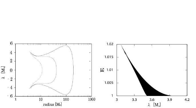
Figure 1: Left: The location of sonic points as a function of the Bernoulli constant ($E$) and specific angular momentum ($\lambda$) in the Schwarzschild geometry. The solid, dashed, dotted lines correspond to $E=1.004$, $1.02$ and $1.1$, respectively. Right: The injection parameters for the existence of a standing shock wave. The shaded region allows the standing shock wave. The adiabatic index is $4/3$ for both panels.

The left panel of Figure 1 shows the locations of the sonic points in Schwarzschild black hole as a function of the Bernoulli constant and specific angular momentum (see also Lu (1986)). As shown in the figure, there are indeed two or three sonic points for some combinations of the Bernoulli constant and angular momentum. The maximum and minimum specific angular momenta are $\lambda_{max}\sim 4.0M_{\ast}$ and $\lambda_{min}\sim 3.2M_{\ast}$, respectively, for the Bernoulli constant $E=1.004$, for example. It should be noted that one of the most important differences between the full GR and the pseudo-Newtonian treatments is the range of the injection parameters that allows the existence of multiple sonic points. As the Bernoulli constant becomes smaller, the maximum specific angular momentum gets larger without limit for the pseudo Newtonian case whereas it is bounded for the full GR case. For the Bernoulli constant that may be typical for massive stellar collapse, e.g. $E=1.003$, the maximum specific angular momentum is larger by about 60% for the pseudo Newtonian approximation than for the full GR treatment. The reason for this difference is that the gravity nearby the black hole is too strong in the pseudo-Newtonian approximation. It should be pointed out that the region of the injection parameters that allows multiple sonic points is not very wide and the above-mentioned difference may be important in considering the implications for astrophysical phenomena.

2.2 The locations of standing shock waves

The sonic points discussed in the previous subsection correspond to the so-called critical points in dynamical system. It is known that the innermost and outermost critical points are of the saddle-type, while the middle critical point is of the center-type. Hence, the transonic accretion flows can be constructed only for the former two critical points. These two transonic flows have the same Bernoulli constant and angular momentum but different entropies, and they can be connected by a standing shock wave, where the Rankine-Hugoniot relations hold:

$$[\,\rho_{0}u^{\mu}\,]\,l_{\mu} = 0,$$ (7)

$$[\,T^{\mu\nu}\,]\,l_{\nu} = 0,$$ (8)

where $l_{\mu}$ is a 4-dimensional vector normal to the shocked surface, and is set to be $l_{\mu}=\left(0,1,0,0\right)$ in axisymmetric steady flows (see also Eq. (23) for the non-axisymmetric perturbations). We use the notation of $[\,Q\,]\equiv Q_{+}-Q_{-}$, where the subscript $(+)$ represents a post-shock quantity and $(-)$ a pre-shock quantity. The Bernoulli constant and specific angular momentum are defined respectively as

$$E \equiv -hu_{t},$$ (9)

$$\lambda \equiv -\frac{u_{\phi}}{u_{t}}.$$ (10)

Since the Bernoulli constant, specific angular momentum and mass flux are unchanged across the shock, we only need to consider the radial component of energy momentum conservation across the shock. Then the Rankine-Hugoniot relation in axisymmetric steady flows can be written as:

$$[\,\rho_{0}hu_{r}u^{r}+p\,] = 0.$$ (11)

In general, there are two possible shock locations, to which we refer as the inner and outer shocks. This is apparent in the right panel of the Figures 1, in which we show the parameter region that allows multiple shock locations. It is well known, however, that the inner shock is unstable against axisymmetric perturbations (Nakayama, 1995), which we have confirmed by our own linear analysis. We have also done numerical simulations with a single grid point in the azimuthal direction, thus suppressing non-axisymmetric modes, and observed that the inner shock is either swallowed by a black hole or moved outwards to be the outer shock after radial perturbations are imposed. On the other hand, we have seen that the outer shock is stable against radial perturbations even if the perturbation amplitude is not necessarily small. In the following, we will consider only the outer shock.

We have constructed several axisymmetric steady accretion flows with an outer shock for different combinations of the adiabatic index and injection parameters, which are summarized in Table 1.

3 Linear Analysis of non-axisymmetric shock instability

Here we give the basic equations and boundary conditions for the linear analysis. The obtained eigen values are later compared with the numerical simulations, and the eigenstates are employed to impose the initial perturbations.

The basic equations are the linearized relativistic continuity and energy-momentum tensor conservation equations (see Eqs. (1) and (2)). We again neglect the $\theta$-component of velocity and all the $\theta$-derivatives and consider the equatorial plane only. Under this assumption, the system equations are written as follows:

$$\partial_{r}f = \frac{i}{\rho_{0(0)}u^{r(0)}}\biggl{\{}\,\rho_{0(1)}u^{t(0)}\sigma+\rho_{0(0)}\left(\omega u^{t(1)}-mu^{\phi(1)}\right)\,\biggr{\}},$$ (12)

$$\partial_{r}q = \frac{i}{\rho_{0(0)}u^{r(0)}h_{(0)}u^{t(0)}}\left(\,\omega p_{1}+\rho_{0(0)}u^{t(0)}h_{(0)}u_{t(0)}\sigma q\,\right),$$ (13)

$$\partial_{r}V_{(1)} = i\frac{u^{t(0)}}{u^{r(0)}}\sigma V_{(1)},$$ (14)

$$\partial_{r}S_{(1)} = i\frac{u^{t(0)}}{u^{r(0)}}\sigma S_{(1)},$$ (15)

where $S$ is entropy and the following notations are used:

$$f \equiv \frac{\rho_{0(1)}}{\rho_{0(0)}}+\frac{u^{r(1)}}{u^{r(0)}},$$ (16)

$$q \equiv \frac{h_{(1)}}{h_{(0)}}+\frac{u_{t(1)}}{u_{t(0)}},$$ (17)

$$V_{(1)} \equiv \omega\left(\,h_{(1)}u_{\phi(0)}+h_{(0)}u_{\phi(1)}\,\right)+m\left(\,h_{(1)}u_{t(0)}+h_{(0)}u_{t(1)}\,\right),$$ (18)

$$\sigma \equiv \omega-m\frac{u^{\phi(0)}}{u^{t(0)}}.$$ (19)

Following the standard procedure of linear stability analysis, the perturbed quantities are assumed to be proportional to $e^{-i\omega t+im\phi}$. All perturbed quantities are calculated from $f,q,V_{(1)}$ and $S_{(1)}$. $V_{(1)}$ and $S_{(1)}$ can be integrated analytically as

$$V_{(1)} = V_{(1)}\biggl{|}_{R}\,\exp\left(\,i\frac{u^{t(0)}}{u^{r(0)}}\sigma\,\right),$$ (20)

$$S_{(1)} = S_{(1)}\biggl{|}_{R}\,\exp\left(\,i\frac{u^{t(0)}}{u^{r(0)}}\sigma\,\right),$$ (21)

where the subscript ’R’ denotes the value evaluated at $r=R$. Thus, we need to integrate numerically only two Eqs. (12) and (13).

These linearized equations can be solved with appropriately setting boundary conditions, which are imposed at the shock surface and inner sonic point. In this study, we assume that the perturbations are confined in the post-shock region and the pre-shock region remains unperturbed. As a result, the outer boundary condition is set at the shock surface. We express the shock radius as follows:

$$R_{sh}=R_{sh(0)}+\eta\exp\left(\,-i\omega t+im\phi\,\right),$$ (22)

where $\eta$ denotes the initial amplitude of shock displacement. Defined as the 4-dimensional vector normal to the shock surface, $l_{\nu}$ can be given as

$$l_{\nu}=\left(i\omega\eta e^{-i\omega t+im\phi},1,0,-im\eta e^{-i\omega t+im\phi}\right).$$ (23)

Using these relations in the Rankine-Hugoniot relations expressed in general as $[\,Q^{\mu}\,]\,l_{\mu}=0$, we can write Eqs. (7) and (8) as

$$[\,Q^{t(0)}\,]i\omega\eta-[\,Q^{\phi(0)}\,]im\eta+[\,Q^{r(1)}\,]=0,$$ (24)

where the following notations are employed:

$$Q^{\mu(0)}\equiv Q^{\mu(0)}\biggl{|}_{R_{sh(0)}},$$ (25)

$$Q^{\mu(1)}\equiv Q^{\mu(1)}\biggl{|}_{R_{sh(0)}}+\eta\left(\frac{d}{dr}Q^{\mu(0)}\right)\biggl{|}_{R_{sh(0)}}.$$ (26)

As mentioned above, we assume that the pre-shock quantities are unperturbed, i.e $\left(Q^{\mu(1)}|_{R_{sh(0)}}\right)_{-}=0$. The explicit forms of these equations are given by

$$\left(\rho_{0(0)}u^{r(1)}\right)_{+}+\left(\rho_{0(1)}u^{r(0)}\right)_{+}+A=0,$$ (27)

$$\biggl{\{}\left(\rho_{0}hu^{t}u^{r}\right)^{(0)}\,\left(\frac{\rho_{0(1)}}{\rho_{0(0)}}+\frac{h_{(1)}}{h_{(0)}}+\frac{u^{t(1)}}{u^{t(0)}}+\frac{u^{r(1)}}{u^{r(0)}}\right)\biggr{\}}_{+}+B=0,$$ (28)

$$\biggl{\{}\left(\rho_{0}h\left(u^{r}\right)^{2}\right)^{(0)}\,\left(\frac{\rho_{0(1)}}{\rho_{0(0)}}+\frac{h_{(1)}}{h_{(0)}}+2\frac{u^{r(1)}}{u^{r(0)}}\right)+p_{(1)}g^{rr}\biggr{\}}_{+}+C=0,$$ (29)

$$\biggl{\{}\left(\rho_{0}hu^{\phi}u^{r}\right)^{(0)}\,\left(\frac{\rho_{0(1)}}{\rho_{0(0)}}+\frac{h_{(1)}}{h_{(0)}}+\frac{u^{\phi(1)}}{u^{\phi(0)}}+\frac{u^{r(1)}}{u^{r(0)}}\right)\biggr{\}}_{+}+D=0,$$ (30)

with the following definitions:

$$A \equiv \biggl{\{}\left(\frac{d}{dr}\rho_{0(0)}u^{r(0)}\right)_{+}-\left(\frac{d}{dr}\rho_{0(0)}u^{r(0)}\right)_{-}\biggr{\}}\,\eta+i\omega\eta\,\biggl{\{}\left(\rho_{0(0)}u^{t(0)}\right)_{+}-\left(\rho_{0(0)}u^{t(0)}\right)_{-}\biggr{\}}$$ (31)

$$-im\eta\,\biggl{\{}\left(\rho_{0(0)}u^{\phi(0)}\right)_{+}-\left(\rho_{0(0)}u^{\phi(0)}\right)_{-}\biggr{\}},$$

$$B \equiv \biggl{\{}\left(\frac{d}{dr}\rho_{0(0)}h_{0}u^{t(0)}u^{r(0)}\right)_{+}-\left(\frac{d}{dr}\rho_{0(0)}h_{0}u^{t(0)}u^{r(0)}\right)_{-}\biggr{\}}\,\eta$$ (32)

$$+i\omega\eta\,\biggl{\{}\left(\rho_{0}h\left(u^{t}\right)^{2}+pg^{tt}\right)^{(0)}_{\!+}-\left(\rho_{0}h\left(u^{t}\right)^{2}+pg^{tt}\right)^{(0)}_{\!-}\biggr{\}}$$

$$-im\eta\,\biggl{\{}\left(\rho_{0}hu^{t}u^{\phi}\right)^{(0)}_{\!+}-\left(\rho_{0}hu^{t}u^{\phi}\right)^{(0)}_{\!-}\biggr{\}},$$

$$C \equiv \biggl{\{}\left(\frac{d}{dr}\left(\rho_{0(0)}h_{(0)}\left(u^{r(0)}\right)^{2}+p^{(0)}g^{rr}\right)\right)_{+}-\left(\frac{d}{dr}\left(\rho_{0(0)}h_{(0)}\left(u^{r(0)}\right)^{2}+p^{(0)}g^{rr}\right)\right)_{-}\biggr{\}}\,\eta$$ (33)

$$+i\omega\eta\,\biggl{\{}\left(\rho_{0}hu^{t}u^{r}\right)^{(0)}_{\!+}-\left(\rho_{0}hu^{t}u^{r}\right)^{(0)}_{\!-}\biggr{\}}$$

$$-im\eta\,\biggl{\{}\left(\rho_{0}hu^{r}u^{\phi}\right)^{(0)}_{\!+}-\left(\rho_{0}hu^{r}u^{\phi}\right)^{(0)}_{\!-}\biggr{\}},$$

$$D \equiv \biggl{\{}\left(\frac{d}{dr}\rho_{0(0)}h_{0}u^{\phi(0)}u^{r(0)}\right)_{+}-\left(\frac{d}{dr}\rho_{0(0)}h_{0}u^{\phi(0)}u^{r(0)}\right)_{-}\biggr{\}}\,\eta$$ (34)

$$+i\omega\eta\,\biggl{\{}\left(\rho_{0}hu^{\phi}u^{t}\right)^{(0)}_{\!+}-\left(\rho_{0}hu^{\phi}u^{t}\right)^{(0)}_{\!-}\biggr{\}}$$

$$-im\eta\,\biggl{\{}\left(\rho_{0}h\left(u^{\phi}\right)^{2}+pg^{\phi\phi}\right)^{(0)}_{\!+}-\left(\rho_{0}h\left(u^{\phi}\right)^{2}+pg^{\phi\phi}\right)^{(0)}_{\!-}\biggr{\}}.$$

As for the inner boundary condition, on the other hand, a regularity condition is imposed at the sonic point. By combining Eqs. (12) to (19), we obtain the differential equation for $u_{r}$, which is written generally as

$$F\left(u_{r}\right)_{,r}=G.$$ (35)

The linearized form of this equation becomes

$$\left(u_{r(1)}\right)_{,r}=\frac{G_{(1)}-F_{(1)}u_{r(0),r}}{F_{(0)}},$$ (36)

where the explicit forms of $F_{(0)}$, $F_{(1)}$ and $G_{(1)}$ are

$$F_{(0)} \equiv \rho_{0(0)}h_{(0)}g^{rr}\biggl{\{}u^{r(0)}u_{r(0)}-\left(b_{s(0)}\right)^{2}\left(1+u^{r(0)}u_{r(0)}\right)\biggr{\}}$$ (37)

$$F_{(1)} \equiv \,\rho_{0(1)}h_{(0)}\left(u^{r(0)}\right)^{2}+\rho_{0(0)}h_{(1)}\left(u^{r(0)}\right)^{2}+2\rho_{0(0)}h_{(0)}u^{r(0)}u^{r(1)}$$ (38)

$$\,-\Gamma g^{rr}\biggl{\{}p_{(1)}\left(1+u^{r(0)}u_{r(0)}\right)+2p_{(0)}u^{r(1)}u_{r(0)}\biggr{\}},$$

$$G_{(1)} \equiv \,\Gamma\left(g^{rr}\!_{,r}+\frac{2}{r}\right)\biggl{\{}\left(p_{(1)}u_{r(0)}+p_{(0)}u_{r(1)}\right)\left(1+u_{r(0)}u^{r(0)}\right)+2p_{(0)}\left(u_{r(0)}\right)^{2}u^{r(1)}\biggr{\}}$$ (39)

$$+\,\frac{1}{2}\biggl{\{}\rho_{0(1)}h_{(0)}u^{r(0)}+\rho_{0(0)}h_{(1)}u^{r(0)}+\rho_{0(0)}h_{(0)}u^{r(1)}\biggr{\}}\biggl{\{}g_{rr,r}\left(u^{r(0)}\right)^{2}+g_{\phi\phi,r}\left(u^{\phi(0)}\right)^{2}+g_{tt,r}\left(u^{t(0)}\right)^{2}\biggr{\}}$$

$$+\,\rho_{0(0)}h_{(0)}u^{r(0)}\biggl{\{}g_{rr,r}u^{r(0)}u^{r(1)}+g_{\phi\phi,r}u^{\phi(0)}u^{\phi(1)}+g_{tt,r}u^{t(0)}u^{t(1)}\biggr{\}}$$

$$+\,i\rho_{0(0)}h_{(0)}u^{r(0)}u^{t(0)}u_{r(1)}\sigma$$

$$+\,i\Gamma p_{(0)}\left(1+u_{r(0)}u^{r(0)}\right)\left(-\omega u^{t(1)}+mu^{\phi(1)}\right)$$

$$-\,iu^{t(0)}p_{(1)}\sigma.$$

$b_{s(0)}$ and $\Gamma$ are the unperturbed sound velocity in the comoving frame and the adiabatic index, respectively. Since $F_{(0)}$ vanishes at the sonic point, we impose the regularity condition there:

$$G_{(1)}-F_{(1)}u_{r(0),r}=0.$$ (40)

4 Numerical Method and Models

The growth of the initial perturbations is computed with a multi-dimensional general relativistic hydrodynamics code, which is based on a modern technique, the so-called high-resolution central scheme (Kurganov & Tadmor, 2000). The details of the numerical scheme are given in Appendix.

We use the Kerr-Schild coordinates with the Kerr parameter being set to be zero, since they have no coordinate singularity at the event horizon and we can put the inner boundary inside the event horizon. This is very advantageous for numerical simulations. We employ a $\Gamma$-law EOS, $p=\left(\Gamma-1\right)\rho_{0}\epsilon$, where $p$ and $\rho_{0}$ and $\epsilon$ are the pressure, rest-mass density, and specific internal energy, respectively.

The computational domain is a part of the equatorial plane with $1.5M_{\ast}\leq r\leq 200M_{\ast}$ and the computation times are $\sim 6\times 10^{4}M_{\ast}$, where $M_{\ast}$ denotes the black hole mass and the unit with $c=G=1$ is used. We employ $600(r)\times 60(\phi)$ grid points. The radial grid width is non-uniform with the grid being smallest, ($\Delta r=0.1M_{\ast}$), at the inner boundary and increasing geometrically by $0.34\%$ per zone toward the outer boundary.

The initial perturbation modes are summarized in Table 1. For Models M1 to M12 we add the $m=1$ mode, where $m$ stands for the azimuthal mode number in $e^{im\phi}$. For Models M1m2 and M1m3, on the other hand, the $m=2,3$ modes are initially imposed, respectively. These models are meant for the study of the initial-mode dependence. In order to investigate the initial-amplitude dependence, we also run Models M1a10 and M1a100, whose initial amplitudes are $10\%$ and $100\%$, respectively. The unperturbed flows for Models M1m2, M1m3, M1a10 and M1a100 are common to those of the other models.

The radial distributions of these modes are obtained by the linear analysis. This is important to compare the linear growth of purely single modes between the linear analysis and numerical simulations, and is one of the differences from Molteni et al. (1999). We choose the most unstable mode for each azimuthal wave number except for M1a100, in which the following perturbation is employed to avoid a velocity larger than the light velocity:

$$v^{r}=v^{r}\!_{sta}\biggl{\{}1+\sin\left(\phi\right)\biggr{\}},$$ (41)

where $v^{r}\!_{sta}$ is the unperturbed radial velocity. The initial perturbations are added to the whole post-shock region, except for Model M1a100, in which the perturbation is imposed to the region between the inner sonic point and the shock again to prevent the flow velocity from being larger than the light velocity.

In the following, we set the black hole mass to be $M_{\ast}=3$M_☉, where $M_{\sun}$ is the solar mass. We have in mind here some applications to astrophysical phenomena such as GRBs and QPOs. Since the formulation is dimensionless, the scaling is quite obvious.

5 Numerical Results by GRHD

In this section, we describe the time evolutions of non-axisymmetric instability obtained by fully dynamical GRHD simulations. In the following analysis, we frequently employ the mode decomposition of the shock surface by the following Fourier transform:

$$a_{m}\left(t\right)=\int_{0}^{2\pi}R_{sh}\left(\phi,t\right)\,e^{im\phi}\,d\phi,$$ (42)

where $R_{sh}\left(\phi,t\right)$ and $a_{m}\left(t\right)$ are the radius of the shock wave as a function of $\phi$ and $t$ and the amplitude of mode $m$ as a function of $t$, respectively.

5.1 Basic Features

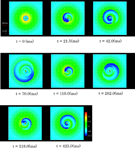
Figure 2: The time evolution of velocity for Model M1. The color contour shows the magnitude of radial velocity. The arrows represent the velocities at their positions. The central region in blue corresponds to the black hole.

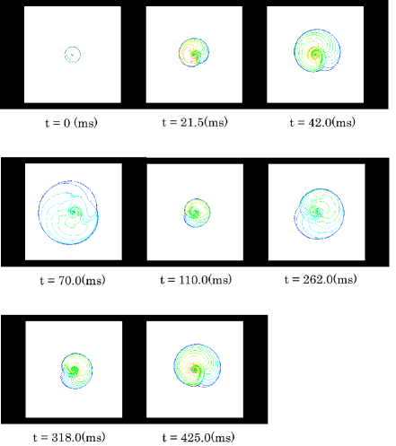
Figure 3: The time evolution of entropy for Model M1.

Figures 2 and 3 show the temporal evolutions of velocity and entropy for the baseline model M1, respectively. The perturbation grows exponentially at the beginning and the shock wave is deformed according to the imposed $m=1$ mode, for which the deformed shock surface rotates progressively, that is, in the direction of the unperturbed flows. Then the shock radius, or the $m=0$ mode, starts to grow. After several revolutions, a spiral arm develops and the instability is saturated with more complex structures. In this non-linear regime, several shocks are generated and collide with each other. As a result of these interactions, the original shock oscillates radially.

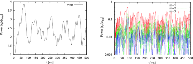
Figure 4: The time evolutions of the $m=0$ mode (left) and the $m=1,2,3$ modes (right).

As given in Table 2, the saturation levels of shock radius, or the $m=0$ mode, differ widely among models. For example, the left panel of Figure 4 shows the time evolution of $m=0$ mode for Model M1. Both large- and small-amplitude oscillations can be seen, which correspond to the periods of $\sim 100$ ms and $\sim 20$ ms, respectively. These two kinds of axisymmetric oscillations are also found in other models. Their characteristics are summarized in Table 2. The growth of $m=0$ mode in the non-linear phase is strongly dependent on the mach number (see Tables 1 and 2 ). i.e., a stronger shock tends to become more unstable against non-axisymmetric perturbations. Although there is no entry to the maximum amplitude of m=0 mode in Table 2 for Model M5, this is not an exception. In fact, the shock is so unstable in this model that it leaves the computational domain soon after the addition of non-axisymmetric perturbations.

On the other hand, the oscillation periods of the non-axisymmetric modes are much shorter in general than those of the axisymmetric ones. Indeed, the right panel of Figure 4 shows the time evolutions of $m=1,2,3$ modes for Model M1. The typical periods range from several to a few dozen milli-seconds.

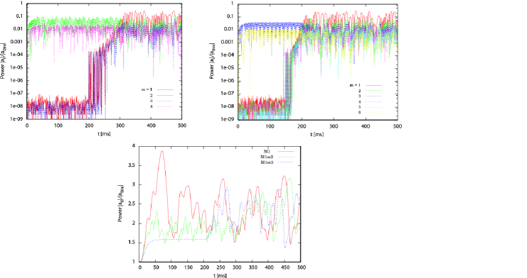
Figure 9: The time evolutions of the amplitudes of various modes. The upper left (right) panel shows the results for Model M1m2 (M1m3). The lower panel displays the evolution of $m=0$ mode for Models M1, M1m2 and M1m3.

In the non-linear phase, the dominant mode is $m=1$ for almost all models. Remarkably, although the initially added perturbations are not the $m=1$ mode in Models M1m2 and M1m3, the non-linear mode couplings lead eventually to the dominance of the $m=1$ mode (see the upper panels of Figure 9).

5.2 Comparison with linear analysis

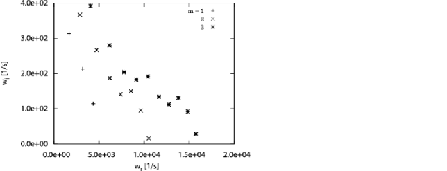
Figure 5: The real and imaginary parts of eigen frequencies for some of the $m=1,2,3$ modes for Model M1.

Equations (12) to (15) with the boundary conditions at the shock surface and sonic point are solved numerically to find eigen modes. Figure 5 shows the real and imaginary parts of eigen frequencies for some of the $m=1,2,3$ modes for Model M1. They are all unstable non-axisymmetric modes. We find, on the other hand, that the axisymmetric perturbations are stable, which is consistent with both the present dynamical simulations and the previous work (Nakayama, 1995). The oscillation periods, which correspond to $\omega_{r}$, are $1.5\sim 3.7$ ms for the most unstable mode in each m-sequence for Model M1, whereas the growth times, which are obtained from $\omega_{i}$, are $2.6\sim 3.2$ ms.

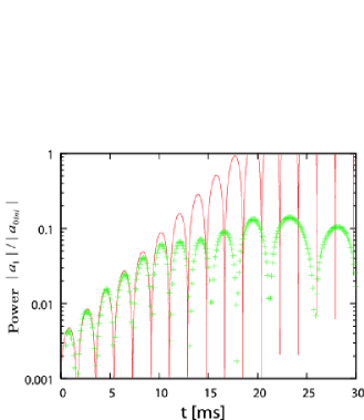
Figure 6: The comparison of the time evolutions of the amplitudes of $m=1$ mode for Model M1 obtained by the linear analysis and dynamical simulation. The red line shows the evolution expected by the linear analysis, while the green crosses are the simulation results.

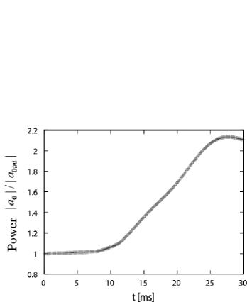
Figure 7: The evolution of the amplitude of $m=0$ mode for Model M1.

Figure 6 shows the comparison of the amplitudes obtained by the linear analysis and dynamical simulations. As can be clearly seen, the oscillation period and growth time are in good agreement between them for the first $10$ ms, which is the linear growth phase. It is also found that after $10$ ms, the result of the dynamical simulation starts to deviate from that of the linear analysis, which indicates the beginning of the non-linear phase. The amplitude is saturated and the oscillation period gets slightly longer. According to Figure 7, which shows the evolution of axisymmetric $m=0$ mode, we find that it starts to grow at $t\sim 10$ ms, leading to the increase of the average shock radius. This is the reason why the oscillation period becomes longer in the non-linear phase.

As mentioned in the previous section and summarized in Table 2, the dominant modes in the non-linear phase are progressive, that is, the deformation pattern rotates in the same direction as the unperturbed flow. This is also true for all the linearly unstable modes. In fact, the linear analysis shows that there is no unstable mode for $m<0$. Note that Yamasaki & Foglizzo (2007) demonstrated by linear analysis for the accretion onto a neutron star that the progressive modes are enhanced and retrogressive ones are suppressed by rotation.

As the specific angular momentum of the unperturbed flow becomes larger, the distance between the shock wave and the inner sonic point gets greater (See Models M1 and M4 in Table 1). According to the linear analysis, the number of unstable modes also increases, whereas the growth time of the most unstable modes becomes longer. This suggests that the larger distance tends to stabilize the non-axisymmetric instability though it is not the only factor for the shock instability. In fact, it is also found that the growth rate of unstable modes is affected by the shock strength, that is, stronger shocks tend to be more unstable.

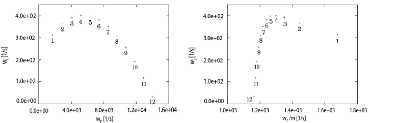
Figure 8: Left: the most unstable eigenfrequency in each mode. Right: the same as in left figure but the horizontal axis is the pattern frequency $\omega_{r}/m$

Finally we show in Figure 8 the most unstable modes for different $m$’s in Model M1. As is clear, the most unstable of all is the $m=4$ mode and the modes with $m>12$ are stable for this model. It is also interesting to note that the real part of eigen frequency for the most unstable modes becomes larger as the mode number $m$ is higher (see the left panel of Figure 8), while the pattern frequency $\omega_{r}/m$ becomes smaller (the right panel of Figure 8).

5.3 Dependence on the initial perturbations

By comparing Models M1, M1a10 and M1a100, we find that the qualitative feature of dynamics are almost the same. In the linear phase, the growth of mode amplitudes is unaffected by the initial condition. Only the duration of the linear phase become shorter as the initial amplitude is larger as expected. The saturation levels do not differ very much among three models. In fact, the non-linear phase is rather chaotic and forgets the difference in the initial condition. It is also important to point out that in spite of the large initial amplitude for Model M1a100, the shock continues to exist. This implies that if the injection parameters are appropriate, a standing shock will exist oscillating violently in the accretion flows into black holes.

Next we show what happens if we impose initially the $m=2$ or $3$ mode instead of the $m=1$ mode, comparing Models M1, M1m2 and M1m3. In the upper panels of Figure 9, we show the time evolutions of the amplitudes for various modes in Models M1m2 (left panel) and M1m3 (right panel).

We first pay attention to the evolution up to $\sim 150$ ms, where the difference is most evident. Note that the linear phase lasts only for $\sim 10$ ms and the non-linear phase thereafter is the focus here. In the left panel, we see the growth and saturation of $m=4$ mode in addition to the original $m=2$ mode. On the other hand, the $m=6$ mode is formed to grow to the saturation in the right panel. Note that the $m=0$ mode is also generated in these models and will be discussed later. These models are produced by the non-linear mode-couplings, which are of quadratic nature, and the other modes with odd $m$ for Model M1m2, for example, are not generated.

After $\sim 150$ ms, however, other modes also emerge and grow to be saturated. These modes are probably generated by numerical noises, having much smaller amplitudes initially and spending longer time in the linear phase. After the saturation of the modes, the dynamics is almost identical for the three models.

In the lower panel of Figure 9, we show the time evolution of the amplitudes of $m=0$ mode for the three models. As mentioned above, the modes are produced by the quadratic mode couplings of the initially imposed modes. Up to $\sim 150$ ms, the evolutions are quite different among them. For Model M1, the amplitude grows to be 4 times larger than the initial value in $\sim 50$ ms and oscillates violently thereafter. On the other hand, the maximum amplitudes are much smaller for Models M1m2 and M1m3, and the following oscillations have much smaller amplitudes. In fact, for Model M1m3 the amplitude becomes almost constant after $\sim 50$ ms. The saturation level is much lower than that of Model M1m2. It is interesting to point out that even though the $m=3$ mode is the unstable in the linear phase (see Figure 5), the average shock radius, or the $m=0$ mode, is most strongly affected by the $m=1$ mode. After $\sim 150$ ms, all modes are saturated and the behavior of the $m=0$ mode becomes almost identical among the different models.

5.4 Dependence on the adiabatic index

In this paper, we employ the simple $\Gamma$-law EOS and so far we have discussed only the case with $\Gamma=4/3$. In reality the EOS will not be so simple and the adiabatic index may not be constant. In order to infer the differences that the EOS may make, we vary the adiabatic index in the the $\Gamma$-law EOS and see the changes in this subsection.

It is the unperturbed accretion flows that are most affected by the change of adiabatic index. It is found that as the adiabatic index becomes larger, both the specific angular momentum and Bernoulli constant that allow the existence of a standing shock wave gets smaller. This is understood as follows. The structure of unperturbed accretion flows and hence the existence of shock are determined by the balance between the attractive gravity and the repulsive centrifugal force and pressure. As the EOS becomes harder, the pressure gets larger and, as a result, the centrifugal force can be reduced. For the same specific angular momentum, on the other hand, the Bernoulli constant can be smaller for harder EOS’s. Note that the Bernoulli constant is a measure of the matter temperature at infinity.

The instability itself is also affected by the change of adiabatic index, since it depends on the structure of unperturbed accretion flows. The results are summarized in Tables 2 and 3. Although it is difficult to find a systematic trend here, the saturation amplitude of the $m=0$ mode appears to be correlated with the Mach number: as the Mach number becomes larger by the change of adiabatic index, the saturation level gets enhanced. It is more important to understand here, however, that the instability does not change qualitatively in spite of the relatively large variation in the injection parameters that allow the existence of the standing shock wave. More thorough investigations of the EOS dependence will be a future task.

5.5 Instability Mechanisms

To gain some insight into the instability mechanism, we calculate some time scales as follows:

$$\tau_{d-c(c)}\equiv\int_{r_{cor}}^{r_{sh}}\left(\,\frac{1}{|v^{r}|}+\frac{1}{C_{s}^{+}}\,\right)\,dr,$$ (43)

$$\tau_{c-c(c)}\equiv\int_{r_{cor}}^{r_{sh}}\left(\,\frac{1}{C_{s}^{-}}+\frac{1}{C_{s}^{+}}\,\right)\,dr,$$ (44)

$$\tau_{d-c(s)}\equiv\int_{r_{inso}}^{r_{sh}}\left(\,\frac{1}{|v^{r}|}+\frac{1}{C_{s}^{+}}\,\right)\,dr,$$ (45)

$$\tau_{c-c(s)}\equiv\int_{r_{inso}}^{r_{sh}}\left(\,\frac{1}{C_{s}^{-}}+\frac{1}{C_{s}^{+}}\,\right)\,dr,$$ (46)

where $r_{inso}$ is the radius of inner sonic point and $C_{s}^{\pm}$ are the outgoing (+) and ingoing (-) sound velocities, respectively, and are given in the observer’s frame for the Schwarzschild geometry as,

$$C_{s}^{\pm}=\Biggl{|}\,\frac{\left(1-b_{s}^{\,2}\right)u^{t}u^{r}\pm\biggl{\{}\large\{\left(1-b_{s}^{\,2}\right)u^{t}u^{r}\large\}^{2}-[\left(1-b_{s}^{\,2}\right)\,\left(u^{t}\right)^{2}\,-\,b_{s}^{\,2}\,g^{tt}][\left(1-b_{s}^{\,2}\right)\,\left(u^{r}\right)^{2}\,-\,b_{s}^{\,2}\,g^{rr}]\biggr{\}}^{\frac{1}{2}}}{\left(1-b_{s}^{\,2}\right)\,\left(u^{t}\right)^{2}\,-\,b_{s}^{\,2}\,g^{tt}}\,\Biggr{|}.$$ (47)

Here $b_{s}$ denotes the sound velocity in the comoving frame. The corotation point of the perturbation is defined as

$$\omega_{r}-m\frac{u^{\phi}\left(r_{cor}\right)}{u^{t}\left(r_{cor}\right)}=0$$ (48)

and its radius is expressed as $r_{cor}$. This investigation is inspired by the previous works (Gu & Foglizzo, 2003; Gu & Lu, 2005) mentioned in the introduction. These time scales and the radius of corotation point for all the models are summarized in Table 3. For comparison, we list the oscillation and growth time scales, which are obtained by linear analysis for the most unstable mode.

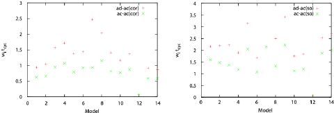
Figure 10: The ratio of the growth rate to the frequencies of advective-acoustic (+) and acoustic-acoustic cycles ($\times$) for all the models. In the left (right) panel, the corotation (inner sonic) point is assumed to be the inner reflection point.

Figure 10 compares the growth times with the cycle periods given by Eqs. (43) to (46) for all the models. It is found that the periods of acoustic-acoustic cycle are closer to the growth times than those of the advective-acoustic cycle, which appears to support the claim by the preceding papers (Gu & Foglizzo, 2003; Gu & Lu, 2005) that the instability is of the Papaloizou-Pringle type. It is important, however, to point out that we can not identify the reflection point clearly (see Figure 10, in which the left (right) panel adopts the corotation (inner sonic) point as the inner reflection point). This is mainly because the wavelengths of the perturbations are rather long. In fact, we estimate the wavelength of acoustic perturbation by

$$\lambda_{w}\equiv\min\left(\frac{2\pi b_{s}}{\omega_{r}}\right),$$ (49)

which should be much smaller than the scale height of the unperturbed flows for the justification of WKB approximations. The wavelength of the dominant unstable mode for each model is given in Table 3. According to this estimation, it is comparable or longer than the scale height. Hence the WKB approximation is not justified at least for these models. Indeed, the reflection point of waves lose its meaning. Incidentally, the WKB approximation may be applicable to higher harmonics. In fact, there are sequences of unstable modes up to m=12 for Model M1, for example, and the wavelengths of their high harmonics are found to be shorter than the scale height. It should be noted, however, that they have smaller growth rates and subdominant in driving the instability. Note also that the above analysis neither approves nor disproves of a particular mechanism in a mathematically rigorous sense. We need further investigation definitely.

6 Implications for Astrophysical Phenomena

In the previous sections, we have found that the standing shock wave in the accretion flow into the Schwarzschild black hole is generally unstable to the non-axisymmetric perturbations and that it oscillates with large amplitudes in the non-linear regime. Here we consider the astrophysical implications of the shock instability, picking up Black Hole QPOs and GRBs as examples.

6.1 Black Hole QPOs

As mentioned already, quasi-periodic oscillations have been observed for a couple of black hole candidates and they are attributed to some activities of the accretion disk around the black hole. The shock oscillation model for black hole QPOs has been investigated by many authors (Das et al., 2003a, b; Chakrabarti et.al., 2004; Aoki et al., 2004; Okuda et al., 2007). Recently, for example, Okuda et al. (2007) performed two-dimensional pseudo-Newtonian numerical simulations of the shock oscillation in the meridian section assuming axisymmetry and taking into account the cooling and heating of gas and the radiation transport. They demonstrated that a quasi-periodically oscillating shock wave is formed around a black hole. They compared the numerical results with the observations for GRS 1915+105 and suggested that the intermediate frequency QPO of this source might be due to the shock instability (Okuda et al., 2007).

Our models are different from those of Okuda et al. (2007). They consider the axisymmetric oscillations whereas we investigate the non-axisymmetric oscillations. We take general relativity fully into account. Besides, we calculate the energy density spectra for the present models. In so doing, we employ the data in the non-linear regime, that is, 100 ms after the onset of computations. Note that the dynamics in the non-linear phase is almost identical in all the models, including the ones, in which the $m=2$ or $3$ mode is initially imposed instead of the $m=1$ mode.

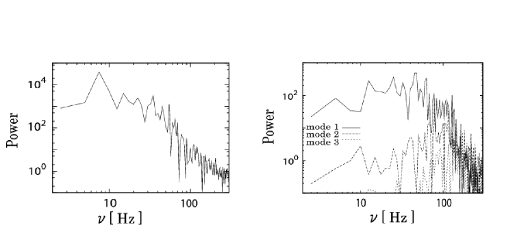
Figure 11: Power spectra of energy density for the $m=0$ mode (left) and $m=1,2,3$ modes (right).

Figure 11 shows the power spectra for the $m=0,1,2,3$ modes in Model M1. It is found that the $m=0$ mode has a quasi-periodic feature around 8 Hz, which corresponds to the period of large oscillations observed for the $m=0$ mode. Although there are some hints of other QPOs, they are much less remarkable. This axisymmetric quasi-periodic oscillation is similar to those found by Okuda et al. (2007). The most important point here, however, is the fact that the quasi-periodicity of $m=0$ mode is induced by the non-axisymmetric instability through the quadratic mode coupling.

Similar quasi-periodic oscillations are found also in other models. Their frequencies depend on the unperturbed flow and, hence, on the Bernoulli constant and specific angular momentum. The quantitative comparison with observations is beyond the scope of this paper, since we have neglected radiative processes, viscosity and, among other things, we have considered only the equatorial plane. It can be mentioned, however, that the non-axisymmetric shock instability is a good candidate of the source of QPOs and further investigations are certainly needed.

6.2 Fluctuations in GRB jets

Long GRBs are currently thought to be associated with massive stellar collapses and the subsequent formation of black holes. Although the central engine remains a mystery, it is widely believed that a highly relativistic jet is somehow produced near the black hole and its kinetic energy is later dissipated in internal shocks at larger distances, emitting gamma rays (see Meszaros (2006) for a recent review). In the so-called ’patchy shell’ model, the jet actually consists of mass shells that have slightly different velocities and collide with each other, generating the internal shock waves. Although the time scale of the velocity fluctuations is thought to be set by the dynamical time scale of the black hole, the exact physical processes producing the velocity variations are unknown at present.

During the collapse of massive stars giving rise to GRBs, a large amount of matter will accrete on a time scale of seconds onto a proto neutron star at first and into a black hole later. If the progenitor is rotating rapidly prior to the collapse (Yoon et al., 2008), the accreting matter will form a disk around the compact object at the center. The accretion disk is expected to be advection-dominated (Popham et al., 1998). We are thus interested in the stability of the accretion flows into the black hole, especially in the accretion-dominated regime. Here we consider the accretion flows with a standing shock wave in them, since the core bounce produces a shock wave, which becomes an standing shock in the core soon after and will continue to exist in the subsequent accretions onto a proto neutron star, the phase just preceding the black hole formation. Even if the bounce shock does not survive, there will be a lot of chances of shock formation as long as the standing shock is robust, since the velocity and pressure of accreting matter are fluctuating in reality.

According to the patchy shell model, gamma rays are emitted when the kinetic energy of ultra-relativistic jet is dissipated in internal shock waves, which are originated from the inhomogeneity of the jet. Although the mechanism of jet formation remains unknown, the black hole is supposed to be involved. The source of the inhomogeneity is also an unsolved problem. If a standing shock wave exists in the accretion flow, for example, as a relic of the shock wave produced at the core bounce, we speculate that the intrinsic instability of the system against non-radial perturbations will be a natural source of fluctuations in the GRBs jet if it is formed from some interactions between the accretion disk and black hole, which is not unlikely (Blandford & Znajek, 1977). It is mentioned incidentally that the recent progenitor models, which could produce GRB (MacFadyen & Woosley, 1999; Heger et al., 2005), predict the injection parameters that are appropriate for the existence of a standing accretion shock. For example, Heger et al. (2005) calculated the evolutions of massive stars, taking into account magnetic fields and obtained the specific angular momentum of several $\times 10^{16}$ cm²/s and the temperature $\lesssim 10^{10}K$ for the matter that will later form an accretion disk. These numbers are just suitable for the existence of a standing shock wave in the accretion disk around a black hole of several M_⊙.

Owing to the non-axisymmetric instability, the mass flux fluctuates very much indeed in our models. In this context, it is interesting to mention that the quasi-periodic oscillation with a period much longer than the dynamical time scale, which we have found in the previous sections, may leave its imprint somehow in the prompt gamma ray emissions or early X-ray afterglows. It is certainly necessary, however, to study possible effects of cooling (Popham et al., 1998) on the instability. The disk thickness we ignored in this paper is also a concern in the future work. We finally mention that the gravitational radiation by the non-radial shock instability may also have interesting implications.

7 Summary and Conclusion

We have investigated the non-axisymmetric shock instability in the accretion disk around Schwarzschild black holes, employing the fully general relativistic hydrodynamic simulations as well as the linear analysis. Both the linear and non-linear phases have been analyzed in detail. We have also given some possible implications for astrophysically interesting phenomena such as Black Hole QPOs and GRBs.

The main findings in the present work are as follows:

(a) The standing shock is generally unstable against non-axisymmetric perturbations, and a spiral arm structure is formed as a result of the growth of instability. It is typically one-armed, implying that the dominant mode in the non-linear phase is the $m=1$ mode.

(b) In the linear phase, the dynamical simulations are in good agreement with the linear analysis in such features as stability, oscillation and growth time scales. The progressive modes, in which the deformed shock pattern rotates in the same direction as the unperturbed flow, are unstable and the retrogressive modes are stable. This is consistent with the previous works.

(c) In the non-linear phase, various modes are produced by non-linear couplings, which are mainly of quadratic nature, and the amplitudes are saturated. The axisymmetric mode is also induced by the non-axisymmetric instability, and the shock radius oscillates with large amplitudes. The oscillation periods become slightly longer than in the linear analysis because of larger shock radii.

(d) Even though strong perturbations are added initially, the shock remains to exist. Hence the disk plus shock system is quite robust in this sense.

(e) The comparison of various cycle time scales with the linear growth times seems to support the claim that the instability is induced by the acoustic-acoustic cycle, although the inner reflection point is not identified unambiguously. It is important to note in this respect that the wavelength of perturbations is longer than the scale height, which does not allow the WKB approximation.

(f) The Black Hole SASI found by Molteni et al. (1999) may be a promising candidate for the sources of the Black Hole QPOs and fluctuations in GRB jets.

In the present study, we have also found that the non-axisymmetric instability is sensitive to the structure of the unperturbed steady flow. The general relativity is important in this respect. It should be stressed that the injection parameters that allow the existence of a standing shock wave are different between the GR and pseudo-Newtonian treatments. In fact, we have found by the direct comparison that the maximum specific angular momentum for the existence of multiple sonic points is different by more than 60% for the Bernoulli constant $E\leq 1.003$.

Note also that the general relativity is indispensable in discussing the accretion into a Kerr black hole, since the frame-dragging will play an important role. This is currently undertaken (Nagakura & Yamada, 2008). For more detailed comparison with observations, it is necessary to include the cooling and heating for GRBs case, and the magnetic field and viscosity for Black Hole QPOs. Last but not least, the discussed simulations including the polar dimension are inevitable.

Appendix A General Relativistic Hydrodynamic Code

Here we describe the GRHD code that are used in this paper. As mentioned already, it is base on the so-called central scheme, which guarantees a good accuracy even if flows include strong shocks and/or high Lorentz factors. Magnetic fields can be also included (DelZanna & Bucciantini, 2002; Shibata & Sekiguchi, 2005; Duez et al., 2005).

Though we do not take into account the evolution of gravitational field, the so-called 3+1 formalism is suitable for hydrodynamics as well. Following Duez et al. (2005), we write the metric in the form

$$ds^{2}=-{\alpha}^{2}dt^{2}+\gamma_{ij}\left(dx^{i}+{\beta}^{i}dt\right)\left(dx^{j}+{\beta}^{j}dt\right),$$ (A1)

where $\alpha$, $\beta^{i}$, and $\gamma_{ij}$ are the lapse, shift vector, and spatial metric, respectively. The basic equations for fluid dynamics in 3+1 form are expressed as:

$$\partial_{t}{\rho}_{\ast}+\partial_{j}\left({\rho}_{\ast}v^{j}\right) = 0,$$ (A2)

$$\partial_{t}S_{i}+\partial_{j}\left(\alpha\sqrt{\gamma}\,T^{j}\!_{i}\right) = \frac{1}{2}\alpha\sqrt{\gamma}\,T^{\alpha\beta}g_{\alpha\beta,i},$$ (A3)

$$\partial_{t}{\tau}+\partial_{i}\left({\alpha}^{2}\sqrt{\gamma}\,T^{0i}-{\rho}_{\ast}v^{i}\right) = s,$$ (A4)

where various variables are defined as follows:

$$v^{j} \equiv \frac{u^{j}}{u^{t}},$$ (A5)

$${\rho}_{\ast} \equiv \alpha\sqrt{\gamma}\,\rho_{0}u^{t},$$ (A6)

$$S_{j} \equiv \alpha\sqrt{\gamma}\,T^{0}\!_{j}={\rho}_{\ast}hu_{j},$$ (A7)

$$\tau \equiv \alpha^{2}\sqrt{\gamma}\,T^{00}-{\rho}_{\ast}={\rho}_{\ast}\alpha hu^{t}-\sqrt{\gamma}\,p-{\rho}_{\ast},$$ (A8)

$$s \equiv \alpha\sqrt{\gamma}\,\biggl{\{}\left(T^{00}\beta^{i}\beta^{j}+2T^{0i}\beta^{j}+T^{ij}\right)K_{ij}-\left(T^{00}\beta^{i}+T^{0i}\right)\partial_{i}\alpha\biggr{\}}.$$ (A9)

In the above equations, $\gamma$ and $K_{ij}$ are the determinant of the three metric and extrinsic curvature, respectively. We refer to $\rho_{\ast}$, $S_{j}$ and $\tau$ as “conserved variables (collectively denoted by $U$)”, whereas $\rho_{0}$, $p$ and $v^{i}$ are called “primitive variables (collectively expressed as $P$)”.

The conserved variables can be calculated directly from the primitive variables via Eqs. (A6), (A7) and (A8). There is no analytical expression for the primitive variables as a function of the conserved variables, on the other hand. Since we update the conserved variables rather than the primitive variables, we must need to solve the latter numerically at each time step because they are necessary for the calculations of the characteristic wave speed at each cell interface as shown later. If we use a $\Gamma$-law EOS, the inversion can be conducted easily as done by Duez et al. (2005). The same method can not be applicable to the general EOS, however. Hence we take a different procedure based on the Newton-Raphson method, which will be explained below.

We first write down a useful relation between $u^{t}$ and $u_{j}$

$$u^{t}=\frac{1}{\alpha}\biggl{\{}1+\gamma^{ij}u_{i}u_{j}\biggr{\}}^{\frac{1}{2}}.$$ (A10)

We define two more quantities as

$$f_{1} \equiv {\rho_{0}}^{2}\gamma\biggl{\{}{{\rho}_{\ast}}^{2}h^{2}+\gamma^{ij}S_{i}S_{j}\biggr{\}}-{{\rho}_{\ast}}^{4}h^{2},$$ (A11)

$$f_{2} \equiv \tau+{\rho}_{\ast}-{\rho}_{\ast}\alpha hu^{t}+\sqrt{\gamma}\,p.$$ (A12)

We then search iteratively for the primitive variables that satisfy $f_{1}=f_{2}=0$. We first guess two thermodynamical quantities $\rho_{0}$ and $p$. Then other thermodynamical quantities can be obtained from the EOS. Next, we obtain $u_{j}$ from Eq. (A7) using $S_{j}$, $\rho_{\ast}$ and $h$, $u^{t}$ is determined by $u_{j}$ from Eq. (A10). Thus the right hand sides of Eqs. (A11) and (A12) are expressed as a function of only two thermodynamical quantities. We solve them by the Newton-Raphson method. The initial guess is obtained from the values at the previous step.

The net flux at the cell interface is given by the approximate solution to the Riemann problem. Our code adopts the HLL (Harten. Lax, and van Leer) flux, which does not require the complete knowledge of the solutions to the Riemann problem but the maximum wave speed in each direction is needed. The first step for calculating the flux is to obtain $P_{R}$ and $P_{L}$, which are the values of primitive variables interpolated to the right- and left-hand side of each cell interface. We have implemented the MUSCL method (HIRSCH, C., 1990) for this purpose. From $P_{R}$ and $P_{L}$, the maximum wave speed on each side of the cell interface, $c_{\pm,R}$ and $c_{\pm,L}$, can be calculated as in Duez et al. (2005).

The HLL flux is then expressed with the maximum wave speeds defined by $c_{+max}\equiv max(0,c_{+,R},c_{+,L})$ and $c_{-max}\equiv max(0,c_{-,R},c_{-,L})$ as

$$f_{int}=\frac{c_{-max}f_{R}+c_{+max}f_{L}-c_{-max}c_{+max}\left(U_{R}-U_{L}\right)}{c_{-max}+c_{+max}},$$ (A13)

where $f_{R}$ and $f_{L}$ are the fluxes calculated with $P_{R}$ and $P_{L}$, respectively. Note that if we define $c_{-max}=c_{+max}=max(0,c_{+,R},c_{+,L},c_{-,R},c_{-,L})$, then $f_{int}$ becomes the local Lax-Friedrichs flux.

Table 1: Model Parameters

	Adiabatic	Bernoulli	Specific Angular	Inner Sonic	Shock Point	Mach Number	Initial	Initial Perturbation
Model	Index   $\Gamma$	Constant   $E$	Momentum $\lambda$	Point $r_{inso}$	$r_{sh}$		Perturbation Mode	Amplitude
M1	$\frac{4}{3}$	1.004	3.43$M_{\ast}$	5.3$M_{\ast}$	16.1$M_{\ast}$	2.4	1	1 %
M2	$\frac{4}{3}$	1.004	3.46$M_{\ast}$	5.2$M_{\ast}$	23.2$M_{\ast}$	2.3	1	1 %
M3	$\frac{4}{3}$	1.004	3.50$M_{\ast}$	5.0$M_{\ast}$	34.8$M_{\ast}$	2.1	1	1 %
M4	$\frac{4}{3}$	1.004	3.56$M_{\ast}$	4.8$M_{\ast}$	78.4$M_{\ast}$	1.5	1	1 %
M5	$\frac{4}{3}$	1.001	3.50$M_{\ast}$	5.1$M_{\ast}$	16.9$M_{\ast}$	4.1	1	1 %
M6	$\frac{4}{3}$	1.005	3.50$M_{\ast}$	5.0$M_{\ast}$	50.2$M_{\ast}$	1.6	1	1 %
M7	1.033	1.13	3.80$M_{\ast}$	4.4$M_{\ast}$	38.7$M_{\ast}$	2.2	1	1 %
M8	1.167	1.02	3.70$M_{\ast}$	4.6$M_{\ast}$	64.2$M_{\ast}$	1.4	1	1 %
M9	1.167	1.02	3.60$M_{\ast}$	5.0$M_{\ast}$	14.0$M_{\ast}$	2.7	1	1 %
M10	1.167	1.03	3.60$M_{\ast}$	5.0$M_{\ast}$	32.4$M_{\ast}$	1.5	1	1 %
M11	1.433	1.001	3.35$M_{\ast}$	5.2$M_{\ast}$	40.6$M_{\ast}$	2.3	1	1 %
M12	1.433	1.004	3.15$M_{\ast}$	6.0$M_{\ast}$	36.5$M_{\ast}$	1.3	1	1 %
M1m2	$\frac{4}{3}$	1.004	3.43$M_{\ast}$	5.3$M_{\ast}$	16.1$M_{\ast}$	2.4	2	1 %
M1m3	$\frac{4}{3}$	1.004	3.43$M_{\ast}$	5.3$M_{\ast}$	16.1$M_{\ast}$	2.4	3	1 %
M1a10	$\frac{4}{3}$	1.004	3.43$M_{\ast}$	5.3$M_{\ast}$	16.1$M_{\ast}$	2.4	1	10 %
M1a100	$\frac{4}{3}$	1.004	3.43$M_{\ast}$	5.3$M_{\ast}$	16.1$M_{\ast}$	2.4	1	100 %

Note. — The locations of inner sonic point and shock surface are determined by the adiabatic index, Bernoulli constant and specific angular momentum. The mach number is calculated in the corotating observer’s frame. $M_{\ast}$ is the mass of the central black hole.

Table 2: Properties of Instability

	dominant mode	maximum amplitude
Model	in non-linear phase	of $m=0$ mode	$\tau_{la}$	$\tau_{sm}$
M1	m=1	3.9	$\approx$100ms	$\approx$20ms
M2	m=1	5.1	$\approx$120ms	$\approx$20ms
M3	m=1	3.2	$\approx$200ms	$\approx$20ms
M4	m=1 or 2	1.3	-	$\approx$ 50ms
M5	m=1	-	-	-
M6	m=1	1.5	$\approx$210ms	$\approx$30ms
M7	m=1	4.5	-	$\approx$50ms
M8	m=1	1.4	$\approx$300ms	$\approx$20ms
M9	m=1	3.5	$\approx$80ms $\approx$20ms
M10	m=1	1.3	-	$\approx$10ms
M11	m=1	4.2	$\approx$300ms	$\approx$60ms
M12	-	-	-	-
M1m2	m=1	3.1	$\approx$100ms	$\approx$20ms
M1m3	m=1	2.9	$\approx$100ms	$\approx$20ms
M1a10	m=1	3.5	$\approx$100ms	$\approx$20ms
M1a100	m=1	4.0	$\approx$100ms	$\approx$20ms

Note. — $\tau_{la}$ ($\tau_{sm}$) is the large- (small-) amplitude oscillation period. The symbol (-) implies no identifications.

Table 3: Cycle Frequencies

	Corotation Point	Oscillation Period	Growth Time	Wavelength of Acoustic Perturbations
Model	$r_{coro}$	$t_{osci}$	$t_{grow}/2\pi$	$\lambda_{w}$	$\tau_{d-c(c)}$	$\tau_{c-c(c)}$	$\tau_{d-c(s)}$	$\tau_{c-c(s)}$
M1	47.7km (10.6$M_{\ast}$)	3.7ms	3.2ms	142.6km (31.7$M_{\ast}$)	3.0ms	2.0ms	6.9ms	5.1ms
M2	64.3km (14.3$M_{\ast}$)	6.4ms	4.8ms	213.7km (47.5$M_{\ast}$)	5.0ms	3.2ms	10.6ms	7.1ms
M3	62.3km (13.9$M_{\ast}$)	5.9ms	8.2ms	171.9km (38.2$M_{\ast}$)	12.9ms	7.8ms	18.3ms	11.3ms
M4	61.2km (13.6$M_{\ast}$)	5.6ms	29.0ms	120.1km (26.7$M_{\ast}$)	49.7ms	31.1ms	55.1ms	33.9ms
M5	50.4km (11.2$M_{\ast}$)	4.1ms	2.4ms	147.6km (32.8$M_{\ast}$)	3.3ms	1.9ms	7.5ms	4.9ms
M6	53.1km (11.8$M_{\ast}$)	4.5ms	17.3ms	114.3km (25.4$M_{\ast}$)	25.0ms	16.1ms	29.0ms	18.6ms
M7	104.8km (23.3$M_{\ast}$)	14.5ms	8.4ms	294.3km (65.4$M_{\ast}$)	20.8ms	7.9ms	159.2ms	18.1 ms
M8	61.2km (13.6$M_{\ast}$)	5.5ms	22.6ms	121.5km (27.0$M_{\ast}$)	46.0ms	26.1ms	56.6ms	30.0ms
M9	43.6km (9.7$M_{\ast}$)	3.1ms	2.2ms	97.2km (21.6$M_{\ast}$)	3.1ms	1.8ms	7.5ms	4.9ms
M10	61.2km (13.6$M_{\ast}$)	5.6ms	11.0ms	157.9km (35.1$M_{\ast}$)	12.8ms	8.5ms	19.3ms	12.3ms
M11	67.5km (15.0$M_{\ast}$)	7.2ms	10.7ms	211.0km (46.9$M_{\ast}$)	14.6ms	9.3ms	19.6ms	12.8ms
M12	44.1km (9.8$M_{\ast}$)	3.5ms	252.2ms	113.8km (25.3$M_{\ast}$)	16.1ms	13.0ms	18.9ms	15.6ms
M1m2	51.7km (11.5$M_{\ast}$)	2.2ms	2.7ms	82.8km (18.4$M_{\ast}$)	2.5ms	1.6ms	6.9ms	5.1ms
M1m3	54.0km (12.0$M_{\ast}$)	1.5ms	2.6ms	58.9km (13.1$M_{\ast}$)	2.2ms	1.5ms	6.9ms	5.1ms

Note. — $t_{osci}$, $t_{grow}/2\pi$ and $\lambda_{w}$ represent the oscillation period, growth time and wavelength of acoustic perturbations, respectively, which are obtained by linear analysis. $\tau_{d-c(c)}$, $\tau_{c-c(c)}$, $\tau_{d-c(s)}$, $\tau_{c-c(s)}$ are obtained from Eqs. (43) to (46), which show the acoustic-acoustic cycle or advective-acoustic cycle between the shock surface and the corotation or inner sonic point.

References

- Aoki et al. (2004) Aoki, S. I., Koide, S., Kudoh, T., Nakayama, K., & Shibata, K. 2004, ApJ, 610, 897
- Iwakami et al. (2008) Iwakami et al. in preparation
- Blandford & Znajek (1977) Blandford, R. D., & Znajek, R. L. 1977, MNRAS, 179, 433
- Blondin et al. (2003) Blondin, J. M., Mezzacappa, A., & DeMarino, C. 2003, ApJ, 584, 971
- Blondin & Mezzacappa (2006) Blondin, J. M. & Mezzacappa, A. 2006, ApJ, 642, 401
- Blondin & Mezzacappa (2007) Blondin, J. M. & Mezzacappa, A. 2007, Nature, 445, 58-60
- Chakrabarti & Molteni (1993) Chakrabarti, S., K., & Molteni, D. 1993, ApJ, 417, 671
- Chakrabarti et.al. (2004) Chakrabarti, S. K., Acharyya, K. & Molteni, D. 2004, A&A, 421, 1
- Das et al. (2003a) Das, T. K., Pendharkar, J. K., & Mitra, S. 2003, ApJ, 592, 1078 (2003a)
- Das et al. (2003b) Das, T. K., Rao, A. R., Vadawale, S. V. 2003, MNRAS, 343, 443 (2003b)
- DelZanna & Bucciantini (2002) Del Zanna, L., & Bucciantini, N. 2002, A&A, 390, 1177
- Duez et al. (2005) Duez, M. D., Liu, Y. T., Shapiro, S. L., & Stephens, B. C. 2005, PrD, 72, 024028
- Foglizzo (2001) Foglizzo, T. 2001, A&A, 368, 311
- Foglizzo (2002) Foglizzo, T. 2002, A&A, 392, 353
- Foglizzo et al. (2006) Foglizzo, T., Scheck, L., & Janka, H.-T. 2006, ApJ, 652, 1436
- Fukue (1987) Fukue, J. 1987, PASJ, 39, 309
- Gu & Foglizzo (2003) Gu, W. M.,& Foglizzo, T. 2003, A&A, 409, 1-7
- Gu & Lu (2005) Gu, W. M.,& Lu, J. F. 2005, MNRAS, 365, 647
- Hawley et al. (1984a) Hawley, J. F., Smarr, L. L., & Wilson, J. R. 1984, ApJ, 277, 296 (1984a)
- Hawley et al. (1984b) Hawley, J. F., Smarr, L. L., & Wilson, J. R. 1984, ApJ, 55, 211 (1984b)
- HIRSCH, C. (1990) HIRSCH, C. 1990, Numerical Computation of Internal and External Flows, Vol2 (Chichester:Wiley)
- Heger et al. (2005) Heger, A., Woosley, S. E., & Spruit, H.C. 2005, ApJ, 626, 350
- Kurganov & Tadmor (2000) Kurganov, A., & Tadmor, E. 2000, J. Comput. Phys., 160, 241
- Laming (2007) Laming, J. M. 2007, ApJ, 659, 1449
- Lu (1986) Lu, J. F. 1985 A&A, 148, 176
- MacFadyen & Woosley (1999) MacFadyen, A., & Woosley, S. E. 1999, ApJ, 524, 262
- Meszaros (2006) Meszaros, P. 2006, Rep. Prog. Phys., 69, 2259
- Molteni et al. (1999) Molteni, D., Toth, G., & Kuznetsov, O. A. 1999, ApJ, 516, 411
- Nagakura & Yamada (2008) Nagakura, H., & Yamada, S., in preparation
- Nakayama (1994) Nakayama, K. 1994, MNRAS, 270, 871
- Nakayama (1995) Nakayama, K. 1995, MNRAS, 281, 226
- Nobuta & Hanawa (1994) Nobuta, K., & Hanawa, T. 1994, PASJ, 46, 2
- Ohnishi et al. (2005) Ohnishi, N., Kotake, K., & Yamada, S. 2006, ApJ, 641, 1018
- Okuda et al. (2007) Okuda, T., Teresi, V., & Molteni, D. 2007, MNRAS, 377, 1431
- Popham et al. (1998) Popham, R., Woosley, S. E., & Fryer, C. 1998, ApJ, 518, 356
- Schek et al. (2004) Scheck, L., Plewa, T., Janka, H.-T., Kifonidis, K., & Muller, E. 2004, PrL, 92, 1103
- Schek et al. (2006) Scheck, L., Kifonidis, K., Janka, H.-T., & Muller, E. 2006, A&A, 457, 963
- Shibata & Sekiguchi (2005) Shibata, M., & Sekiguchi, Y. 2005, PrD, 72,044014
- Yamasaki & Foglizzo (2007) Yamasaki, T., & Foglizzo, T. 2007, submitted ApJ, (arXiv:astro-ph/0710.3041v1)
- Yoon et al. (2008) Yoon, S. C., Langer, N., Cantiello, M., Woosley, S. E., & Glatzmaier, G. A. 2008, Proceedings IAU Symposium No. 250, (arXiv:astro-ph/0801.4362)