Also at ]Institute for Scientific Interchange, Viale Settimio Severo 65, I-10133 Torino, Italy

Fidelity approach to the disordered quantum XY model

Abstract

We study the random XY spin chain in a transverse field by analyzing the susceptibility of the ground state fidelity, numerically evaluated through a standard mapping of the model onto quasi-free fermions. It is found that the fidelity susceptibility and its scaling properties provide useful information about the phase diagram. In particular it is possible to determine the Ising critical line and the Griffiths phase regions, in agreement with previous analytical and numerical results.

Introduction.– In the last few years concepts borrowed from quantum information theory have proven useful in characterizing the critical behavior of quantum many-body systems AmFaOs . In particular, a geometric approach to the study of quantum phase transitions (QPTs), i.e. the fidelity analysis, has been shown to be an effective way of characterizing distinct phases of quantum systems ZaPa ; ZaGiCo ; CVZ ; YoLiGu ; ZhBa ; ZhZhLi ; Zh . Previously, the fidelity approach has been applied to a variety of homogeneous systems. In this work we extend these studies to disordered quantum systems. Specifically, we investigate the behavior of the fidelity susceptibility of the disordered XY model in a transverse field. It is well known that the presence of quenched disorder can have drastic effects on critical properties. The appearance of new universality classes and novel states of matter such as the Griffiths phase are two important examples Fis1 ; Fis2 ; Gri ; Sac . The aim of the present work is to show what can be inferred about the physics of the disordered quantum system from the properties of the fidelity susceptibility.

The Hamiltonian of the disordered XY chain is given by

$$H=-\sum_{i=0}^{L-1}\left(\frac{1+\gamma_{i}}{2}\sigma_{i}^{x}\sigma_{i+1}^{x}+\frac{1-\gamma_{i}}{2}\sigma_{i}^{y}\sigma_{i+1}^{y}+\lambda_{i}\sigma_{i}^{z}\right),$$ (1)

where $\sigma_{i}^{\left\{x,y,z\right\}}$ are Pauli spin matrices, and $\gamma_{i}$ and $\lambda_{i}$ are sets of independent random coupling and field variables with distributions $\pi(\gamma_{i})$ and $\rho(\lambda_{i})$. Note that due to gauge symmetry the Hamiltonian (1) can be chosen to have only positive couplings and fields. This model can be mapped onto a system of quasi-free fermions with periodic boundary conditions, and an exact expression for the fidelity susceptibility is obtained which depends explicitly on the random parameters characterizing the ground state of the system. In this work, we investigate the statistical properties of the fidelity susceptibility CVZ ; YoLiGu for relevant regions of parameter space.

Gaussian distributions are used for the random variables,

$$\pi(x_{i})=\rho(x_{i})=\frac{1}{\sigma\sqrt{2\pi}}\exp\left\{{-\frac{1}{2}\left(\frac{x_{i}-x}{\sigma}\right)^{2}}\right\},$$ (2)

where $x_{i}$ is either the field or the coupling at position $i$ on the chain, $x$ is the respective average value and $\sigma^{2}$ is the variance.

Previous Results.– The pure XY chain has been analytically solved in LiScMa . In the absence of disorder two different quantum phase transitions are present. Following the standard notation, we refer to the QPT driven by the transverse magnetic field $\lambda$ as the Ising transition, and to the QPT driven by the coupling parameter $\gamma$ as the anisotropy transition. The Ising transition separates a ferromagnetic ordered phase from a paramagnetic quantum-disordered phase, whereas the anisotropy critical line is the boundary between a ferromagnet ordered along the $x$ direction and a ferromagnet ordered along the $y$ direction.

A major improvement in the understanding of the effect of disorder on the physics of quantum magnets has been achieved with the use of the strong-disorder renormalization group technique (SDRG) by Dasgupta and Ma DasMa , and further developed by Fisher Fis1 ; Fis2 . The correctness of this method has been corroborated both by numerics HaRiDa ; YoRi and analytic exact studies McK ; BuMc . In the work of McKenzie and Bunder McK ; BuMc the critical behavior of the disordered XY chain in a transverse field has been studied using a mapping to random-mass Dirac equations. The properties of the solutions of these equations imply the disappearance of the anisotropy transition in the presence of disorder. Furthermore, Griffiths phases are predicted to appear both around the Ising critical line and the anisotropy $\gamma=0$ line.

For $\gamma=1$ the XY random chain is closely related to the random transverse-field Ising chain (RTFIC), which is a prototypical model for disordered quantum systems. Since it is representative of the universality class of Ising transitions for all values of $\gamma$, let us briefly review what is known for this model. The Hamiltonian of the RTFIC is $H=-\sum_{i=0}^{L-1}\left[J_{i}\sigma_{i}^{x}\sigma_{i+1}^{x}+h_{i}\sigma_{i}^{z}\right],$ where $J_{i}$ and $h_{i}$ are random couplings and fields respectively. The system is at criticality when the average value of the field equals the average value of the coupling. Using the SDRG one obtains that, at the quantum critical point, the time scale $\tau$ and the length scale $L$ are related by $\ln{\tau}\sim L^{1/2}$. This results in an infinite value for the dynamical exponent $z$ at criticality. The distribution of the logarithm of the energy gap, $\ln{\epsilon}$, at criticality broadens with increasing system size, in accordance with the scaling relation $\ln{\epsilon}\sim-L^{1/2}$ YoRi . In the vicinity of the critical point the distribution of relaxation times is broad due to Griffiths singularities. This region of the parameter space, the Griffiths phase, is characterized by a dynamical exponent $z$ which depends on the distance from the critical point. This dependence is one of the hallmarks of the Griffiths phase.

Method.– The main idea of the fidelity approach is to detect QPTs through enhanced orthogonalization rates between ground states $|\Psi(x)\rangle$ nearby in parameter space. The orthogonalization is signaled by a drop in the fidelity, $F(x,x+\Delta x)\equiv\left|\langle\Psi(x)|\Psi(x+\Delta x)\rangle\right|$, at the critical point. The fidelity susceptibility is a related quantity with a more transparent physical meaning YoLiGu ; CVZ , and whose behavior is more suitable for numerical analysis. It is defined as

$$\chi(x)=\lim_{\Delta x\rightarrow 0}\frac{-2\ln{F(x,x+\Delta x)}}{\Delta x^{2}}.$$ (3)

In YoLiGu it was shown that $\chi$ is related to the dynamic structure factor of the relevant operator associated with the transition. A generalization of this result, valid for the so-called geometric tensor, has been given in CVZ .

Previous works have characterized the pure XY spin chain using the fidelity approach ZaPa ; ZaCoGi ; ZaGiCo ; CoGiZa and the quantum Chernoff bound AbJaZa . The mapping of the spin model onto the quasi-free fermion Hamiltonian LiScMa ,

$$H=\sum_{i,j=1}^{L}c^{\dagger}_{i}A_{ij}c_{j}+\frac{1}{2}\sum_{i,j=1}^{L}\left(c^{\dagger}_{i}B_{ij}c^{\dagger}_{j}+H.c.\right),$$ (4)

yields an explicit BCS-like form for the ground state $|\Psi\rangle=\mathcal{N}\exp{\left(\frac{1}{2}\sum_{j,k=1}^{L}c_{j}^{\dagger}G_{jk}c_{k}^{\dagger}\right)}|0\rangle,$ where $\mathcal{N}$ is a normalization factor.

The fidelity of the ground states evaluated at slightly different parameter values (coupling or magnetic field) $x$ and $x+\Delta x$ has a simple analytical expression. Defining the matrix $Z(x)\equiv A(x)-B(x)$ and the unitary part of the polar decompositions of $Z(x)$ and $\tilde{Z}\equiv Z(x+\Delta x)$ as $T(x)$ and $\tilde{T}\equiv T(x+\Delta x)$, respectively, the fidelity can be written as

$$F(Z,\tilde{Z})=\sqrt{|\det{\frac{T+\tilde{T}}{2}}|}.$$ (5)

Note that the matrix $G$ defining the ground state is simply the Cayley transform of $T$ CoGiZa .

In the following, we will use an alternative expression for the fidelity susceptibility, obtained in the limit of small $\Delta x$,

$$\chi(x)=\frac{1}{8}\|\partial_{x}T\|_{F}^{2},$$ (6)

with $\|\cdot\|_{F}$ the Frobenius norm. Eq. (6) is obtained from (5) via standard algebra. We have numerically evaluated the fidelity susceptibility using (6) for relevant regions of parameter space of the disordered XY model. The numerical analysis has been performed on two sets of system sizes, i.e. {128, 256, 512}, and {400, 410, …, 500} in steps of 10. We have taken 50,000 disorder realizations for all sizes except for those larger than 400, in which case we used 10,000 realizations.

Results.– We consider the Hamiltonian (1), where the couplings $\gamma_{i}$ and the transverse fields $\lambda_{i}$ are independent random variables with Gaussian distributions centered around $\lambda\equiv\left[\lambda_{i}\right]_{\textrm{ave}}$ and $\gamma\equiv\left[\gamma_{i}\right]_{\textrm{ave}}$, both with standard deviation $\sigma$. $\left[\cdot\right]_{\textrm{ave}}$ denotes the arithmetic mean over the disorder realizations.

A scaling analysis has been performed using arguments first developed in CVZ . Following that reference, we can express the fidelity susceptibility as an integral in imaginary time $\chi=\int_{-\infty}^{\infty}d\tau\tau G(\tau),$ where $G(\tau)=\theta(\tau)\ll\partial_{x}H(\tau)\partial_{x}H(0)\gg$ is the connected correlation function of the conjugate operator in the Hamiltonian associated with the driving parameter in the transition, and $\theta$ is the Heaviside step function. For example, in the case of the Ising transition we have $G(\tau)=\theta(\tau)\ll\sum_{i,j}\sigma_{i}^{z}(\tau)\sigma_{j}^{z}(0)\gg$. The average fidelity susceptibility can then be written as $\left[\chi\right]_{\textrm{ave}}=\int_{-\infty}^{\infty}d\tau\tau\left[G(\tau)\right]_{\textrm{ave}}\sim L^{\Delta_{\chi}}$, where the finite-size scaling dimension $\Delta_{\chi}$ of $\left[\chi\right]_{\textrm{ave}}$ is given by $\Delta_{\chi}=2z+2-2\Delta_{O}$ CVZ . $\Delta_{O}$ is the scaling dimension of the QPT conjugate operator ($\sum_{i}\sigma_{i}^{z}$ in the case of the transition driven by $\lambda$), and in general $\Delta_{O}$ depends on the parameters $\gamma$ and $\lambda$.

For the XY chain without disorder, in the quantum critical regions $\chi$ scales as $\chi\sim L^{2}$, whereas away from the critical region $\chi\sim L$. Since for finite system sizes the quantum critical region has a finite width, $\Delta_{\chi}$ is $1$ for all but a narrow range of $\lambda$ (or $\gamma$), having a maximum of $2$ for $\lambda=1$ ($\gamma=0$).

With this disorder-free behavior in mind, we now study $\left[\chi\right]_{\textrm{ave}}$ about the Ising transition, driven by the coupling $\lambda$. In our numerical studies we have focused on the case of the RTFIC, where $\gamma=1$. Qualitatively all of our results on the critical behavior of the fidelity susceptibility hold true for other values of $\gamma$, since the universality class of the model does not change in the range $\gamma\in\left(0,1\right]$.

Fig. 1(a) shows $\left[\chi\right]_{\textrm{ave}}$ as a function of $\lambda$ for the clean case and $\sigma=0.1,0.3$ disorder strengths. The averaged fidelity susceptibility displays a local maximum at the Ising critical point, which for the disordered case is shifted slightly away from the clean value of $\lambda=1$ due to finite size effects. Fig. 1(b) shows $\Delta_{\chi}(\lambda)$, the finite-size scaling dimension of $\left[\chi\right]_{\textrm{ave}}$, for the same set of disorder strengths. The disorder leads to a broadening in the peak of $\Delta_{\chi}$, which is consistent with the presence of a Griffiths phase. Note that far from the Ising critical point $\left[\chi\right]_{\textrm{ave}}$ scales strictly extensively, while in the vicinity of the critical point the scaling becomes superextensive. For the weaker noise this scaling is nearly quadratic, as in the clean case, while with stronger noise the maximum scaling dimension is correspondingly reduced. Qualitatively, the reduction of the maximum scaling dimension may be ascribed to the presence of rare regions whose extent effectively determines the critical behavior. The linear extension of rare regions is smaller than the overall system size determining the critical behavior in the clean case.

Figure 1: Ising transition at $\gamma=1$. (a) Average fidelity susceptibility, $\left[\chi\right]_{\textrm{ave}}$, for $L=512$ and $10^{4}$ realizations, with varying disorder strengths $\sigma\in\{0,0.1,0.3\}$, (b) the associated finite-size scaling dimension $\Delta_{\chi}$ of $\left[\chi\right]_{\textrm{ave}}$, (c) probability distribution of $\ln\chi$ at the Ising transition for system sizes $L=128,256,512$ and disorder $\sigma=0.1$, (d) distribution of $\ln\chi$ away from the Ising transition for the same disorder and range of system sizes.

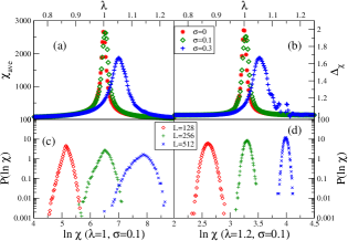
In Fig. 1(c) and (d) we plot the distribution of the fidelity susceptibility over many realizations at the Ising critical point and away from it, for system sizes $L=128,256$, and $512$. We choose to plot the distribution of $\ln\chi$ instead of $\chi$ itself because, in analogy to other physical quantities, the presence of disorder greatly broadens the distribution. As the system size increases, note that the probability density function of $\ln\chi$ broadens for $\lambda=1$, but becomes narrower away from criticality. Indeed, this broadening behavior persists for a range of values of $\lambda$ about the critical point. This is typical of disordered systems, and is analogous to the absence of self-averaging of some physical observables.

The Griffiths phase around the Ising critical point can be detected by looking at the scaling dimension of the fidelity susceptibility and at the properties of the distribution of $\ln\chi$, in accordance with the relation $\Delta_{\chi}=2z+2-2\Delta_{O}$. The following analysis of the region about the anisotropy line further supports this conclusion.

Figure 2: Elimination of anisotropy transition at $\gamma=0$ due to disorder. (a) Average fidelity susceptibility $\left[\chi\right]_{\textrm{ave}}$, near $\gamma=0$ for $L=500$, $\lambda=0.2$, $\sigma=0.1$, and $10^{4}$ realizations. (b) Finite-size scaling dimension of $\left[\chi\right]_{\textrm{ave}}$ (in this case $\gamma=0.036$), (c) probability distribution of $\ln\chi$ at $\gamma=0$ and at the value of $\gamma$ corresponding to the maximum of $\left[\chi\right]_{\textrm{ave}}$, (d) distribution of $\ln\chi$ far away from the anisotropy line, where the finite-size scaling is extensive.

Figure 3: Average fidelity susceptibility for various disorder strengths $\sigma\in\{0,0.1,0.2,0.3\}$, with fixed system size $L=400$. Here $\lambda=0.5$, and the derivative in Eq. (6) is taken along $\gamma$.

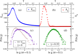
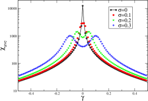
Although for the disordered XY model the $\gamma=0$ line is not critical, as it is in the pure case McK ; BuMc , the presence of Griffiths singularities still has highly non-trivial effects on the fidelity susceptibility in the vicinity of $\gamma=0$, as shown in Fig. 2(a). Specifically, in the presence of disorder the peak in $\left[\chi\right]_{\textrm{ave}}(\gamma)$ splits into two peaks, symmetrical about $\gamma=0$. Note that $\gamma=0$ is a special case for the XY chain. With zero anisotropy and noise only in the field $\lambda_{i}$, Bunder and McKenzie BuMc showed that the density of states does not diverge at zero energy. This implies that this point is not critical and does not belong to a Griffiths phase. We observe similar behavior with disorder in both the field and anisotropy. At $\gamma=0$ the fidelity susceptibility scales only extensively, as it does in the non-critical region. This suggests that the $\gamma=0$ point does not belong to the Griffiths phase, having characteristics of a point which is non-critical and away from any Griffiths phase. This is further corroborated by the non-monotonic dependence on $\gamma$ of the associated scaling dimension shown in Fig. 2(b). At $\gamma=0$, one finds $\Delta_{\chi}=1$, whereas in the interval $0<\gamma<0.075$ the scaling dimension $\Delta_{\chi}(\gamma)$ exhibits a non-universal dependence on the driving parameter $\gamma$, indicating the presence of a Griffiths regime. Note that the observed maximum is not to be seen as an indication of a QPT. Rather, it originates from the competition between the scaling properties of $\chi$ in the Griffiths phase and at the $\gamma=0$ line. In Figs. 2(c) and (d), we show $P(\ln\chi)$ at $\gamma=0$, at the point where $\chi(\gamma)$ and $\Delta_{\chi}(\gamma)$ both peak, and far away from the anisotropy line. In analogy to the Ising transition, the probability distribution function in the Griffiths regime is broad and asymmetric due to absence of self-averaging, whereas far away from it its shape is symmetric and its distribution is much narrower. To complete the discussion of the effects of disorder on the anisotropy transition in Fig. 3 we plot the average fidelity susceptibility for a fixed system size and various disorder strengths, including the clean case. Notice that as the disorder strength is increased, the original peak disappears and the new maxima in the fidelity susceptibility are symmetrically located around the $\gamma=0$ line, at a distance which increases with disorder. Much like the Ising transition, the maximum value of the fidelity susceptibility decreases with increased disorder. We believe that this can be explained again in terms of the extension of rare regions.

Conclusions.– In this work we have applied the fidelity approach to the study of the disordered XY chain in an external magnetic field. We have found that the fidelity susceptibility is able to provide the phase diagram for this model. In the case of the Ising transition, we obtain results which are consistent with what is already known in the literature. In the parameter region around the $\gamma=0$ line the scaling analysis of the fidelity susceptibility shows the disappearance of the QPT and the emergence of a Griffiths phase, in accordance with similar analytical and numerical results. As far as we know, this result has not been obtained before for this distribution of disorder both in the couplings and in the fields. This is nontrivial, since it is known that choosing a different parametrization for the disorder can modify the critical behavior McK .

We plan to further investigate the relevance of disorder on the fidelity susceptibility in future works. Other aspects that will be studied with more details are the extent of the Griffiths phase together with its dependence on disorder strength and the probability distribution of disorder.

We thank H. Saleur and L. Campos Venuti for helpful discussions. Computation for the work described in this paper was supported by the University of Southern California Center for High Performance Computing and Communications. We acknowledge financial support by the National Science Foundation under grant DMR-0804914.

References

- (1) L. Amico, R. Fazio, A. Osterloh and V. Vedral, Rev. Mod. Phys. 80, 517 (2008)
- (2) P. Zanardi and N. Paunkovic, Phys. Rev. E 74, 031123 (2006)
- (3) P. Zanardi, P. Giorda and M. Cozzini, Phys. Rev. Lett. 99, 100603 (2007)
- (4) L. Campos Venuti and P. Zanardi, Phys. Rev. Lett. 99, 095701 (2007)
- (5) W. L. You, Y. W. Li and S. J. Gu, Phys. Rev. E 76, 022101 (2007)
- (6) H.-Q. Zhou and J.P. Barjaktarevic, arXiv:cond-mat/0701608
- (7) H.-Q. Zhou, J.-H. Zhao and B. Li, arXiv:0704.2940
- (8) H.-Q. Zhou, arXiv:0704.2945
- (9) S. Sachdev, Quantum Phase Transitions (Cambridge University Press, 1999)
- (10) D.S. Fisher, Phys. Rev. Lett. 69, 534 (1992)
- (11) D.S. Fisher, Phys. Rev. B 51, 6411 (1995)
- (12) R.B. Griffiths, Phys. Rev. Lett 23, 17 (1969)
- (13) E. Lieb, T. Schultz and D. Mattis, Ann.Phys. 16, 407 (1961)
- (14) C. Dasgupta and S.K. Ma, Phys. Rev. B 22, 1305 (1980)
- (15) S. Haas, J. Riera and E. Dagotto, Phys. Rev. B 48, 13174 (1993)
- (16) A.P. Young and H. Rieger, Phys. Rev. B 53, 8486 (1996)
- (17) R.H. McKenzie, Phys. Rev. Lett. 77, 4804 (1996)
- (18) J.E. Bunder and R. H. McKenzie, Phys. Rev. B 60, 344 (1999)
- (19) M. Cozzini, P. Giorda and P. Zanardi, Phys. Rev. B 75, 014439 (2007)
- (20) P. Zanardi, M. Cozzini and P. Giorda, J. Stat. Mech. L02002 (2007)
- (21) D.F. Abasto, N.T. Jacobson, and P. Zanardi, Phys. Rev. A 77, 022327 (2008)