Classical energy-momentum tensor renormalization via effective field theory methods

Abstract

We apply the Effective Field Theory approach to General Relativity, introduced by Goldberger and Rothstein, to study point-like and string-like sources in the context of scalar-tensor theories of gravity. Within this framework we compute the classical energy-momentum tensor renormalization to first Post-Newtonian order or, in the case of extra scalar fields, up to the (non-derivative) trilinear interaction terms: this allows to write down the corrections to the standard (Newtonian) gravitational potential and to the extra-scalar potential. In the case of one-dimensional extended sources we give an alternative derivation of the renormalization of the string tension enabling a re-analysis of the discrepancy between the results obtained by Dabholkar and Harvey in one paper and by Buonanno and Damour in another, already discussed in the latter.

I Introduction

We consider in this work the classical renormalization of the Energy-Momentum Tensor (EMT) of fundamental particles and strings due to their interaction with long range fundamental fields, including standard gravity. The gravitational self-energy of a massive body for instance, arises because of gravitons’ self-interactions, it can be described as an effective renormalization of the massive body EMT and it is fully classical having its analog in Newtonian physics. Such self-interactions, even if they involve point-like particles, are not divergent when gravity is present, as on general grounds General Relativity imposes a lower limit on the size of massive objects: their Schwartzchild radii.

In the case of one-dimensional extended objects like strings, no horizon analog is present and no fundamental lower limit can be imposed on their size: classical contributions to the EMT due to self-interactions of gravity can (and do indeed) diverge in this case. Letting the source size shrink to zero and keeping fixed other physical parameters like mass and charge (and eventually neglecting gravity), usually one encounters infinities, or equivalently, physical quantities depending critically on the source size. Dirac Dirac emphasized that the cutoff dependence of the energy of the electromagnetic field sourced by an electron can be absorbed by an analog dependence of the bare electron mass, to provide a finite, physically observable invariant mass. However the usual way to consider mass renormalization is by considering the virtual process of emission and reabsorption of a massless fields, like for mass renormalization of the electron in standard electrodynamics, rather then a renormalization of the EMT, i.e. of the particle coupling to gravity, as we are going to do here. The above mentioned virtual processes are usually considered in the context of quantum field theory, but they show their effects also classically, when heavy, non-dynamical, non-propagating sources are considered, as we will show.

In order to compute these quantities we make use of the the formalism introduced in Goldberger:2004jt ; Goldberger:2007hy , which is an effective field theory (EFT) method borrowed from particle physics, where it originated from studying non-relativistic bound state problems in the context of quantum electro- and cromo-dynamics eff-qcd ; Luke:1999kz ; for this reason, it has been coined Non Relativistic General Relativity (NRGR) (see also Damour:1995kt for the first appplication of field theory techniques to gravity problems). Here we apply NRGR in the framework of scalar-tensor theories of gravity for computing next-to-leading order corrections to the EMT renormalization, which in turn define, via the usual Einstein equations, the profile of the graviton generated by the sources.

An example of such a renormalization has been worked out in BjerrumBohr:2002ks for point particles in the GR case and by Dabholkar:1989jt ; Buonanno:1998kx for string-like sources coupled to an extra scalar, the dilaton, and an anti-symmetric tensor, the axion. See also Lund:1976ze ; Battye:1994qa ; Quashnock:1990wv for the string sources interacting with axionic and gravitational fields. We find particularly worth of interest the different analysis performed in Dabholkar:1989jt ; Buonanno:1998kx , leading to apparently conflicting result for the string-tension renormalization. The explanation of the discrepancy is actually given already in Buonanno:1998kx , but here we re-analyize such discrepancy with the fresh insight available thanks to NRGR.

The plan of the paper is as follows. In sec. II we summarize the basic ingredients of NRGR and set the notation for the case at study. In sec. III we apply EFT methods to a model where a scalar and the standard graviton field mediate long range interactions, to compute the effective EMT of a massive body. In sec. IV we present the analogous computation for a one-dimensional-extended object in four dimensions. Finally we draw our conclusions in sec. V.

II Effective field theory

We start by describing the basis of NRGR: in doing so we closely follow the thorough presentation given in Goldberger:2004jt , to which we refer for more details, with the exception of the metric signature, as we adopt the “mostly plus” convention: $\eta_{\mu\nu}\equiv(-,+,+,+)$.

In order to be able to exploit the manifest velocity-power counting, which is at the heart of PN expansion, we must first identify the relevant physical scales at stake. If, for simplicity, we restrict to binary systems of equal mass objects it is enough to introduce one mass scale $m$ and two parameters of the relative motion, namely the separation $r$ and the velocity $v$. It turns out that, up to the very last stages of the inspiral, the evolution of the system can be modelled to sufficiently high accuracy by non-relativistic dynamics, i.e. the leading order potential between the two bodies is the Newtonian one. The virial theorem then allows to relate the three afore-mentioned quantities according to

$$v^{2}\sim\frac{G_{N}m}{r}$$ (1)

(where $G_{N}$ is the ordinary gravitational constant) and tells that an expansion in the (square of the) typical three-velocity of the binary is at the same time an expansion in the strength of the gravitational field.

The compact objects being macroscopic, they can be considered fully non-relativistic ($v<<c$) so that from a field theoretical point of view, and with scaling arguments in mind, the binary constituents are non-relativistic particles endowed with typical four-momentum of the order $p_{\mu}\sim(E\sim mv^{2},{\bf p}\sim m{\bf v})$ (boldface characters are used to denote 3-vectors). Concerning the motion of the bodies subject to mutual gravitational potential, it is convenient to consider only the potential gravitons, i.e. those responsible for binding the system as they mediate instantaneous interactions: their characteristic four-momentum $k_{\mu}$ will thus be of the order

$$k_{\mu}\sim(k^{0}\sim\frac{v}{r},{\bf k}\sim\frac{1}{r})$$

so that these modes are always off-shell ($k_{\mu}k^{\mu}\neq 0$).
When a compact object emits a single graviton, momentum is effectively not conserved and the non-relativistic particle recoils of a fractional amount roughly given by

$$\frac{|\delta{\bf p}|}{|{\bf p}|}\simeq\frac{|{\bf k}|}{|{\bf p}|}\simeq\frac{\hbar}{L}\,,$$

where $L\sim mvr$ is the angular momentum of the system: it is clear that for macroscopic systems such quantity is negligibly small. To summarize, an EFT approach describes massive compact objects in binary systems as non-dynamical, background sources of point-like type: quantitavely this corresponds to having particle world-lines interacting with gravitons. The action we consider is then given by

$$\mathcal{S}=\mathcal{S}_{EH}+\mathcal{S}_{pp}\,,$$ (2)

where the first term is the usual Einstein-Hilbert action

$$\mathcal{S}_{EH}=2M^{2}_{Pl}\int d^{4}x\sqrt{-g}\ R(g)\,,$$ (3)

with the Planck mass defined (non canonically) as $M^{-2}_{Pl}\equiv 32\pi G_{N}\simeq 1.2\times 10^{18}$GeV, and the second term is the point particle action

$$\mathcal{S}_{pp}=-m\int d\tau=-m\int\sqrt{-g_{\mu\nu}dx^{\mu}dx^{\nu}}\,,$$ (4)

in which $g_{\mu\nu}$ is the metric field that we write as $g_{\mu\nu}\equiv\eta_{\mu\nu}+h_{\mu\nu}$ . To make the graviton kinetic term invertible, one should also include a gauge fixing term like

$$\mathcal{S}_{gf}=-M^{2}_{Pl}\int d^{4}x\ \Gamma_{\mu}\Gamma^{\mu}\,,$$ (5)

with $\Gamma_{\mu}\equiv\partial^{\nu}h_{\mu\nu}-1/2\,\partial_{\mu}h^{\nu}_{\nu}$ .

We now parametrize the metric following Kol:2007bc , instead of Goldberger:2004jt , as

$$g_{\mu\nu}=\left(\begin{array}[]{cc}-e^{2\varphi}&-e^{2\varphi}a_{j}\\ -e^{2\varphi}a_{i}&\quad e^{-2\varphi}\gamma_{ij}-e^{-2\varphi}a_{i}a_{j}\\ \end{array}\right)\,,$$ (8)

where $\mu,\nu=0,..,3$ and $i,j=1,2,3$. We define $\gamma^{ij}$ as the inverse matrix of $\gamma_{ij}$, so that $\gamma^{ij}\equiv\left(\gamma^{-1}\right)_{ij}$ and $a^{i}\equiv\gamma^{ij}a_{j}$ . It is also useful to introduce $\varsigma_{ij}\equiv\gamma_{ij}-\delta_{ij}$ (so that $\varsigma^{ij}=\varsigma_{ij}$ to first order) and $\varsigma\equiv\varsigma_{ij}\delta^{ij}$. Then, to quadratic order, the following action for non-canonically normalized fields is obtained

$$\left.\mathcal{S}_{EH}\right|_{\rm quadratic}+\mathcal{S}_{gf}=-\frac{M_{Pl}^{2}}{2}\int dt\,d^{3}{\bf x}\left[\partial_{\mu}\varsigma_{ij}\partial^{\mu}\varsigma_{ij}-\frac{1}{2}\partial_{\mu}\varsigma\partial^{\mu}\varsigma+8\partial_{\mu}\varphi\partial^{\mu}\varphi-2\partial_{\mu}a_{i}\partial^{\mu}a_{i}\right]\,.$$ (9)

The non-relativistic parametrization of the metric (8) allows to write down all the terms that do not involve time derivatives in a simple way

$$\mathcal{S}_{EH}|_{static}=2M_{Pl}^{2}\int dt\,d^{3}{\bf x}\sqrt{-\gamma}\left[R(\gamma)-2\partial_{i}\varphi\partial_{j}\varphi\,\gamma^{ij}+\frac{1}{4}e^{4\varphi}F_{ij}F_{kl}\gamma^{ik}\gamma^{jl}\right]\,,$$ (10)

where $F_{ij}\equiv\partial_{i}a_{j}-\partial_{j}a_{i}$ is the usual field strength tensor.
The canonically normalized fields $\sigma_{ij},\phi,A_{i}$ can be defined as

$$\begin{array}[]{ccl}\sigma_{ij}&\equiv&M_{Pl}\,\varsigma_{ij}\,,\\ \phi&\equiv&2\sqrt{2}M_{Pl}\,\varphi\,,\\ A_{i}&\equiv&\sqrt{2}M_{Pl}\,a_{i}\,.\end{array}$$ (14)

The only interaction term we will need, as it will be explained, is the cubic one $\sigma\phi^{2}$ given by

$$\left.\mathcal{S}_{EH}\right|_{\sigma\phi^{2}} = \displaystyle\frac{1}{2M_{Pl}}\int dt\,d^{3}{\bf x}\left[\partial_{i}\phi\partial_{j}\phi\left(\delta_{ik}\delta_{jl}-\frac{1}{2}\delta_{ij}\delta_{kl}\right)\sigma_{kl}\right]\,.$$ (15)

The world-line coupling to the graviton thus reads

$$\begin{array}[]{rl}\mathcal{S}_{pp}=-m\displaystyle\int d\tau&=\displaystyle-m\int dt\ e^{\phi/(2\sqrt{2}M_{Pl})}\sqrt{\left(1-\frac{A_{i}}{\sqrt{2}M_{Pl}}v^{i}\right)^{2}-e^{-\sqrt{2}\phi/M_{Pl}}\gamma_{ij}v^{i}v^{j}}\\ &\simeq\displaystyle-m\int dt\ e^{\phi/(2\sqrt{2}M_{Pl})}\left(1-\frac{1}{2}v^{2}+\frac{\phi}{2\sqrt{2}M_{Pl}}-\frac{A_{i}}{\sqrt{2}M_{Pl}}v^{i}+\ldots\right)\,.\end{array}$$ (18)

The propagators we use are given by the following non-relativistic expressions, as we are treating the time derivatives in the kinetic terms as perturbative contributions,

$$\begin{array}[]{ccl}\displaystyle\rnode{s1}{\sigma}_{ij}(t,{\bf k})\rnode{s2}{\sigma}_{kl}(t^{\prime},{\bf k}^{\prime})&=&\displaystyle(2\pi)^{3}\delta(t-t^{\prime})\delta^{(3)}({\bf k}-{\bf k}^{\prime})\frac{i}{{\bf k}^{2}}P_{ij,kl}{\psset{nodesep=2.0pt,angle=-90.0,armA=4.0pt,armB=4.0pt}\ncbar{s1}{s2}}\\ \displaystyle\rnode{a1}{A}_{i}(t,{\bf k})\rnode{a2}{A}_{j}(t^{\prime},{\bf k}^{\prime})&=&\displaystyle(2\pi)^{3}\delta(t-t^{\prime})\delta^{(3)}({\bf k}-{\bf k}^{\prime})\frac{i}{{\bf k}^{2}}\delta_{ij}{\psset{nodesep=2.0pt,angle=-90.0,armA=4.0pt,armB=4.0pt}\ncbar{a1}{a2}}\\ \displaystyle\rnode{f1}{\phi}(t,{\bf k})\rnode{f2}{\phi}(t^{\prime},{\bf k}^{\prime})&=&\displaystyle(2\pi)^{3}\delta(t-t^{\prime})\delta^{(3)}({\bf k}-{\bf k}^{\prime})\frac{i}{{\bf k}^{2}}{\psset{nodesep=2.0pt,angle=-90.0,armA=4.0pt,armB=4.0pt}\ncbar{f1}{f2}}\\ \\ \end{array}$$ (23)

where

$$P_{ij,kl}\equiv\frac{1}{2}\left(\delta_{ik}\delta_{jl}+\delta_{il}\delta_{jk}-2\delta_{ij}\delta_{kl}\right)\,.$$ (24)

As far as we are only concerned in scaling we can set $k\sim 1/r$, $t\sim r/v$ and, by virtue of the virial theorem (1), $m/M_{Pl}\sim\sqrt{Lv}$. We can then immediately estimate what are the scalings of the contributions to the scattering amplitude of two massive objects: each of the three diagrams reported in fig. 1, for instance, contributes to such process. By assigning a factor $[\frac{m}{M_{Pl}}dt\,d^{3}{\bf k}]$ to a graviton-worldline coupling not involving velocity, a factor $[\delta(t)\delta^{(3)}({\bf k}){\bf k}^{-2}]$ for each propagator, and a factor $[\frac{{\bf k}^{2}}{M_{Pl}}dt\,\delta^{(3)}({\bf k})\left(d^{3}{\bf k}\right)^{3}]$ for a three-graviton vertex, the following scaling laws can be associated to the different contributions of fig. 1:

$$\begin{array}[]{rcl}(a)&\sim&\displaystyle\left(\frac{m}{M_{Pl}}\right)^{2}\left[dt\,d^{3}{\bf k}\right]^{2}\left[\delta(t)\delta^{(3)}({\bf k}){\bf k}^{-2}\right]\sim L\,,\\ (b)&\sim&\displaystyle\left(\frac{m}{M_{Pl}}\right)^{3}\left[dt\,d^{3}{\bf k}\right]^{3}\left[\delta(t)\delta^{(3)}({\bf k}){\bf k}^{-2}\right]^{3}\left[\frac{{\bf k}^{2}}{M_{Pl}}dt\,\delta^{(3)}({\bf k})\left(d^{3}{\bf k}\right)^{3}\right]\sim Lv^{2}\,,\\ (c)&\sim&\displaystyle\left(\frac{m}{M_{Pl}}\right)^{2}\left[dt\,d^{3}{\bf k}\right]^{2}\left[\delta(t)\delta^{(3)}({\bf k}){\bf k}^{-2}\right]^{4}\left[\frac{{\bf k}^{2}}{M_{Pl}}dt\,\delta^{(3)}({\bf k})\left(d^{3}{\bf k}\right)^{3}\right]^{2}\sim v^{4}\,.\end{array}$$

Even if we are actually dealing with a classical field theory, it is interesting to give a look at the scalings in powers of $\hbar$. To restore $\hbar$’s one can apply the usual rule that relates the number $\mathcal{I}$ of internal graviton lines (graviton propagators) to the number $\mathcal{V}$ of vertices and the number $\mathcal{L}$ of graviton loops

$$\mathcal{L}=\mathcal{I}-\mathcal{V}+1\,;$$ (25)

then, taking into account that each internal line brings a power of $\hbar$ and each interaction vertex a $\hbar^{-1}$ from the interaction Lagrangian, the total scaling for diagrams where the only external lines are massive particles is $\hbar^{{\cal L}-1}$. According to this rule the third diagram of fig. 1 involves one more power of $\hbar$ than the first two. The diagram with a graviton loop is then suppressed with respect to the Newtonian contribution, apart from some powers of $v$, by a factor $\hbar/L\ll 1$, whereas the second diagram in fig. 1 is a 1PN contribution which does not involve any power of $\hbar$. Equivalently one can notice that since the massive object is not propagating (there is no kinetic term in the Lagrangian for such a source), the 1PN diagram is not a loop one.

(a) Newton                     (b) 1PN                  (c) Quantum loop

Figure 1: Contributions to the scattering amplitude of two massive objects. From left to right the diagrams represent respectively the leading Newtonian approximation, a classical contribution to the 1PN order and a negligible quantum 1-loop diagram.

These scaling arguments remain unchanged when other particles are added, like a scalar field, and/or another mass scale is introduced Porto:2007pw , as we will discuss in sec. III, provided that the virial relation (1) correctly accounts for the leading interaction.

III Effective energy-momentum tensor in scalar-gravity theory: the point particle case

The usual way to obtain an effective action $\Gamma$ out of a fundamental action $\mathcal{S}_{fund}$ is by integrating out the degrees of freedom we do not want to propagate to infinity according to the formal rule

$$e^{i\Gamma}\equiv\int{\mathcal{D}}\Phi\,e^{i\mathcal{S}_{fund}}\,,$$ (26)

where $\Phi$ denotes the generic field to integrate out.

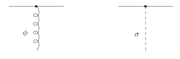
Figure 2: Feynman diagrams describing the gravitational contributions to the effective energy-momentum tensor of a particle at Newtonian level according to the parametrization (8) used for the metric.

In practice this non-perturbative integration is replaced by a perturbative computation, performed with the aid of Feynman diagrams like those of fig. 1 which shows some contributions to the effective action of two particles interacting gravitationally. At lowest order (Newtonian interaction) the diagram in fig. 1(a) represents the term responsible for the Newtonian $1/r$ potential between two massive objects. Stripping away one of the two external lines in this diagram an amplitude for the coupling of a single particle to a graviton is obtained: this amplitude is linear in the external graviton wave-function and defines the effective EMT of the particle. Thus at Newtonian level the two diagrams in fig. 2 give the following contributions to the effective action

$$\begin{array}[]{rl}\displaystyle\Gamma^{(0)}=\Gamma_{\phi}^{(0)}+\Gamma_{\sigma}^{(0)}&=\displaystyle\frac{1}{2\sqrt{2}M_{Pl}}\int\phi(x)\left[T_{00}(x)+T_{ij}(x)\delta_{ij}\right]\,d^{4}x\\ &\displaystyle=\frac{m}{2\sqrt{2}M_{Pl}}\int\phi(t,{\bf x_{p}}(t))\,dt\,,\end{array}$$ (29)

where ${\bf x_{p}}$ is the three-vector of the position of the source particle and use has been made of the Newtonian value of the EMT defined as usual as

$$T_{\mu\nu}(x)\equiv\frac{-2}{\sqrt{-g}}\left.\frac{\delta\mathcal{S}}{\delta g^{\mu\nu}(x)}\right|_{g_{\mu\nu}=\eta_{\mu\nu}}\,.$$ (30)

Note that the contribution from $\Gamma^{(0)}_{\sigma}$ is vanishing as the $\sigma_{ij}$ part of the metric field does not couple directly to a static massive source for which $T_{ij}(x)=0$, $T_{00}(x)=m\delta^{(3)}({\bf x}-{\bf x_{p}})$.

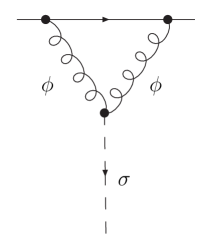
Figure 3: Feynman diagram describing the gravitational contribution to the effective energy-momentum tensor of a particle at first post-Newtonian order according to the parametrization used for the metric (8).

The second diagram in fig. 1 is a representative contribution of the 1PN corrections to the Newtonian potential between two particles. Stripping away again one of the two external particle lines the diagram showed in fig. 3 is obtained, whose contribution to the effective action at next-to-leading order is

$$\begin{array}[]{rl}\displaystyle\Gamma^{(I)}_{\sigma}=&\displaystyle\frac{1}{M_{Pl}}\int d^{4}x\,\sigma_{ij}(x){T^{ij}}^{(I)}(x)=\frac{1}{M_{Pl}}\int dt\,\frac{d^{3}{\bf q}}{\left(2\pi\right)^{3}}\sigma_{ij}(t,-{\bf q}){T^{ij}}^{(I)}(t,{\bf q})e^{i{\bf q}\cdot{\bf x}_{p}}\\ =&\displaystyle\frac{m^{2}}{8M^{3}_{Pl}}\int dt\frac{d^{3}{\bf q}}{\left(2\pi\right)^{3}}\frac{d^{3}{\bf k}}{\left(2\pi\right)^{3}}\frac{k^{i}k^{j}-k^{i}q^{j}}{{\bf k}^{2}\left({\bf k}-{\bf q}\right)^{2}}\left(\delta^{l}_{i}\delta^{m}_{j}-\frac{\delta_{ij}\delta^{lm}}{2}\right)\sigma_{lm}(t,-{\bf q})e^{i{\bf q}\cdot{\bf x}_{p}}\\ =&\displaystyle\frac{m^{2}}{2^{10}M^{3}_{Pl}}\int dt\,\frac{d^{3}{\bf q}}{(2\pi)^{3}}\sigma_{ij}(t,-{\bf q})\left(-\delta^{ij}q+\frac{q^{i}q^{j}}{q}\right)e^{i{\bf q}\cdot{\bf x}_{p}}\,,\end{array}$$ (34)

where $q\equiv\sqrt{{\bf q}\cdot{\bf q}}$ and we have used eqs.(89). The analogous quantity for $\phi$ vanishes as there is no $\phi^{3}$ vertex, see eq.(10). Incidentally, we note that the EMT obtained from eq. (34) is transverse, consistently with the request that the effective EMT has to be conserved order by order (see Sundrum:2003yt for an interesting discussion of scalar gravity at interacting level).

Another check of the correctness of our result can be obtained by reconstructing the metric out of this effective EMT. The linearized equations of motion for gravity give

$$\phi(t,{\bf k})=-\frac{1}{{\bf k}^{2}}\left.\frac{\delta\Gamma_{\phi}}{\delta\phi(t,{\bf k})}\right|_{\phi=0=\sigma_{ij}}$$ (35)

which, using the first of eqs.(94), allows to compute the metric component $\varphi$ according to

$$\varphi(x)\equiv\frac{\phi(x)}{2\sqrt{2}M_{Pl}}=-\frac{m}{8M_{Pl}^{2}}\int\frac{d^{3}{\bf k}}{\left(2\pi\right)^{3}}\frac{e^{i{\bf k}\cdot\left({\bf x}-{\bf x_{p}}\right)}}{{\bf k}^{2}}=-\frac{G_{N}m}{r}\,,$$ (36)

where $G_{N}$ has been reinstated in the final result and $r\equiv|{\bf x}-{\bf x_{p}}|$. Analogously, for $\varsigma_{ij}$ one has

$$\varsigma_{ij}(t,{\bf k})=-\frac{1}{{\bf k}^{2}}\frac{1}{M_{Pl}}P_{ij;kl}\left.\frac{\delta S}{\delta\sigma^{kl}(t,{\bf k})}\right|_{\phi=0=\varsigma_{ij}}$$ (37)

which, again using eqs.(94), leads to

$$\begin{array}[]{rl}\displaystyle\varsigma_{ij}(t,x)=&\displaystyle P_{ij;kl}\int\frac{d^{3}{\bf k}}{\left(2\pi\right)^{3}}\frac{m^{2}}{2^{10}M_{Pl}^{4}}\left(\delta^{kl}k-\frac{k^{k}k^{l}}{k}\right)\frac{1}{{\bf k}^{2}}e^{-i{\bf k}\cdot\left({\bf x}-{\bf x_{p}}\right)}=\\ =&\displaystyle-\frac{\left(G_{N}m\right)^{2}}{r^{2}}\left(\delta_{ij}-\frac{x_{i}x_{j}}{r^{2}}\right)\,.\end{array}$$ (40)

Given the metric parametrization (8) we obtain

$$\begin{array}[]{rcl}\displaystyle g_{00}&=&\displaystyle-1+\frac{2G_{N}m}{r}-2\frac{\left(G_{N}m\right)^{2}}{r^{2}}\\ \displaystyle g_{0i}&=&0\\ \displaystyle g_{ij}&=&\displaystyle\left(1+\frac{2G_{N}m}{r}+\frac{\left(G_{N}m\right)^{2}}{r^{2}}\right)\delta_{ij}+\frac{\left(G_{N}m\right)^{2}}{r^{2}}\frac{x^{i}x^{j}}{r^{2}}\end{array}$$ (44)

which is the Schwarzschild metric to 1PN order in the harmonic gauge, see BjerrumBohr:2002ks .

Let us now consider an extra degree of freedom with respect to ordinary gravity, that is a massive scalar field $\psi$ whose action is given by

$$\mathcal{S}_{\psi}=-\frac{1}{2}\int d^{4}x\sqrt{-g}\left[g^{\mu\nu}\partial_{\mu}\psi\,\partial_{\nu}\psi+m_{\psi}^{2}\psi^{2}+\lambda\psi^{3}\right]\;,$$ (45)

where a cubic self-interaction has been allowed. The interaction with the gravitational field $\sigma_{ij}$, embodied by the trilinear term $\psi\psi\sigma$, can be derived from the kinetic term, namely

$$\left.\mathcal{S}_{\psi}\right|_{\psi\psi\sigma}=\frac{1}{2M_{Pl}}\int dt\,d^{3}{\bf x}\,\partial_{i}\psi\partial_{j}\psi\left(\sigma^{ij}-\frac{1}{2}\delta^{ij}\sigma\right)\,.$$ (46)

There are no trilinear terms such as $\phi\psi\psi$ or $\phi\phi\psi$ because of the specific metric parametrization we chose (8). The field $\psi$ is assumed to couple to matter in a metric type in analogy with (18):

$$\mathcal{S}^{\prime}_{pp}=-me^{\alpha\psi/\left(2\sqrt{2}M_{Pl}\right)}\int d\tau\quad,$$

for some dimensionless parameter $\alpha$. Therefore the tree-level coupling of $\psi$ to matter at lowest order is very similar to the diagram on the left of fig. 2:

$$\Gamma^{(0)}_{\psi}=\frac{\alpha\,m}{2\sqrt{2}M_{Pl}}\int\psi(t,{\bf x_{p}}(t))\,dt\,.$$ (47)

At next-to-leading order we have two possible contributions. The first comes from a diagram like that of fig. 3 where the two $\phi$’s are replaced with two $\psi$’s: the amplitude is almost the same as eq. (34), apart from an extra factor $\alpha^{2}$. The second contribution comes from the cubic $\psi$ self-interaction, depicted in the diagram of fig. 4:

$$\Gamma^{(I)}_{\psi}=\frac{\lambda m^{2}\alpha^{2}}{64\pi M^{2}_{Pl}}\int dt\int\frac{d^{3}{\bf q}}{(2\pi)^{3}}e^{i{{\bf q}\cdot{\bf x_{p}}}}\psi(t,{\bf q})\frac{1}{q}\arctan{\left(\frac{q}{2m_{\psi}}\right)}\,.$$ (48)

Note that at high momentum transfer ($q\gg m_{\psi}$) the integrand goes as $q^{-1}$, whereas in the gravity case (34) we had $T_{ij}^{\sigma}(q)\propto q$: this difference leads to an effective potential due to the $\psi$mediation which has a logarithmic profile, rather than the $1/r^{2}$ behavior typical of 1PN terms in Einstein gravity derived in Porto:2007pw ; at low momenta ($q\ll m_{\psi}$) the Yukawa suppression takes place as usual.

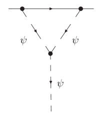
Figure 4: Feynman diagram representing the self-interaction contribution of the massive scalar field $\psi$ to the energy-momentum tensor of a particle at next-to-leading order.

IV Effective energy-momentum tensor: string

In the case of a one-dimensional extended source we consider the Nambu-Goto string with action $\mathcal{S}_{s}$ given by

$$\mathcal{S}_{s}=\mu\int_{\Sigma}\sqrt{-\gamma}\ e^{\alpha\Phi/\left(\sqrt{2}M_{Pl}\right)}\,d\tau d\sigma-\frac{\beta\mu}{2\sqrt{2}M_{Pl}}\int_{\Sigma}\partial_{\alpha}x^{\mu}\partial_{\beta}x^{\nu}\epsilon^{\alpha\beta}B_{\mu\nu}\,d\tau d\sigma\,,$$ (49)

where $\gamma\equiv{\rm det}\gamma_{\alpha\beta}$, with $\gamma_{\alpha\beta}\equiv\partial_{\alpha}x^{\mu}\partial_{\beta}x^{\nu}g_{\mu\nu}$, $x^{\mu}$ are coordinates in the 4-dimensional space, $\sigma$ and $\tau$ are the coordinates on the world-sheet $\Sigma$ spanned by the string in its temporal evolution. Such an action describes a fundamental string interacting with gravity via a string tension $\mu$, with a scalar field $\Phi$ through a coupling $\alpha\mu/(\sqrt{2}M_{Pl})$ and with the antisymmetric tensor $B_{\mu\nu}$ through the coupling $\beta\mu/(2\sqrt{2}M_{Pl})$. In this notation a supersymmetric string corresponds to $\alpha=\beta=1$.
The convention for indeces is the following: $\alpha,\beta$ denote the two directions parallel to the world-sheet while $\mu,\nu,\ldots$ are generic 4-dimensional indeces, then Latin letters $i,j,\ldots$ denote 3-space indeces and we will use $a,b$ or $c$ to denote the (two) spatial dimensions orthogonal to the string.
The action $\mathcal{S}_{f}$ determining the dynamics of the fields is

$$\mathcal{S}_{f}=\int d^{4}x\sqrt{-g}\left[2M_{Pl}^{2}R-\frac{1}{2}\left(\partial\Phi\right)^{2}-\frac{1}{12}e^{-\sqrt{2}\alpha\Phi/M_{Pl}}H_{\mu\nu\rho}H^{\mu\nu\rho}\right]\,,$$ (50)

where $H_{\mu\nu\rho}\equiv\partial_{\mu}B_{\nu\rho}+\partial_{\rho}B_{\mu\nu}+\partial_{\nu}B_{\rho\mu}$. The only new propagator we will need with respect to the point-particle study is

$$\rnode{b1}{B}_{\mu\nu}(t,{\bf k})\rnode{b2}{B}_{\rho\sigma}(t^{\prime},{\bf k^{\prime}})=\frac{1}{2}\left(\eta_{\mu\rho}\eta_{\nu\sigma}-\eta_{\mu\sigma}\eta_{\nu\rho}\right)\left(2\pi\right)^{3}\delta(t-t^{\prime})\delta^{(3)}({\bf k}-{\bf k}^{\prime})\frac{i}{{\bf k}^{2}}\,.{\psset{nodesep=2.0pt,angle=-90.0,armA=4.0pt,armB=4.0pt}\ncbar{b1}{b2}}$$ (51)

Analogously to diagrams in fig. 2, the effective action for the linear coupling to the string source of the fields $\phi$, $\sigma_{ij}$, $\Phi$ and $B_{\mu\nu}$ is $\Gamma^{(0)}=\Gamma^{(0)}_{\phi}+\Gamma^{(0)}_{\sigma_{ij}}+\Gamma^{(0)}_{\Phi}+\Gamma^{(0)}_{B_{\mu\nu}}$ with

$$\begin{array}[]{rcl}\Gamma^{(0)}_{\phi}&=&\displaystyle\int\varphi\left(T_{00}+T_{ij}\delta^{ij}\right)\,d^{4}x=0\,,\\ \Gamma^{(0)}_{\sigma_{ij}}&=&\displaystyle\int\varsigma_{ij}T^{ij}\,d^{4}x=-\frac{\mu}{M_{Pl}}\int_{\Sigma}\sigma_{11}(x(\tau,\sigma))\,d\tau d\sigma\,,\\ \Gamma^{(0)}_{\Phi}&=&\displaystyle\frac{\alpha}{2\sqrt{2}M_{Pl}}\int\Phi\left(T_{00}-T_{ij}\delta^{ij}\right)\,d^{4}x=\frac{\alpha\mu}{\sqrt{2}M_{Pl}}\int_{\Sigma}\Phi(x(\tau,\sigma))\,d\tau d\sigma\,,\\ \Gamma^{(0)}_{B_{\mu\nu}}&=&\displaystyle\frac{\beta\mu}{2\sqrt{2}M_{Pl}}\int_{\Sigma}\partial_{\alpha}x^{\mu}\partial_{\beta}x^{\nu}\epsilon^{\alpha\beta}B_{\mu\nu}\,d\tau d\sigma=\frac{\beta\mu}{\sqrt{2}M_{Pl}}\int_{\Sigma}B_{01}(x(\tau,\sigma))\,d\tau d\sigma\,,\end{array}$$ (56)

where use has been made of the explicit parametrization of a static string: $x^{0}=\tau$, $x^{1}=\sigma$, and of the definition (30) for the string EMT $T^{s}_{\mu\nu}$ giving

$$T_{\mu\nu}^{s}={\rm diag}(\mu,-\mu,0,0)\delta^{(2)}(x^{a})\,.$$ (57)

Following the same reasoning as in sec. III, the contributions to the renormalization of the effective EMT due to the dilaton and the antisymmetric tensor interaction can be computed, see fig. 5. We thus restrict to those trilinear interaction terms involving a graviton field, either a $\phi$ or a $\sigma$, as an external line (in a completely analogous way the renormalization of the $\Phi$ and $B_{\mu\nu}$ coupling could be computed). We then have:

$$\begin{array}[]{rl}\displaystyle\mathcal{S}_{3}=\frac{1}{2M_{Pl}}&\displaystyle\int dt\,d^{3}{\bf x}\left\{\frac{1}{2}\left[\partial_{i}\Phi\partial_{j}\Phi\left(\delta^{il}\delta^{jm}-\frac{1}{2}\delta^{ij}\delta^{lm}\right)\sigma_{lm}\right]+\right.\\ &\displaystyle\left.\!\!\!\!\!\frac{1}{2}\left[\partial_{i}B_{01}\partial_{j}B_{01}\left(\delta^{il}\delta^{jm}+\delta^{ij}\delta^{l1}\delta^{m1}-\frac{1}{2}\delta^{ij}\delta^{lm}+\delta^{il}\delta^{j1}\delta^{m1}+\delta^{jm}\delta^{i1}\delta^{l1}\right)\sigma_{lm}\right]\right\}\,,\end{array}$$ (60)

where we have specified the antisymmetric tensor polarization indices to ”$01$” , as this is the only polarization involved in this interaction, and omitted rewriting the terms coming from the pure gravity sector, i.e. $\sigma^{3}$ and $\phi^{2}\sigma$, because they read the same as in (10).

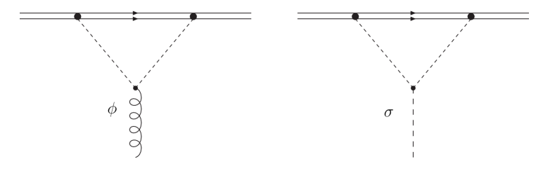
Figure 5: Diagrams reproducing the coupling to $\phi$ (curly line) and to $\sigma_{ij}$ (long-dashed), or the effective energy-momentum tensor, of a string at next to lowest order in interaction. The diagram on the left vanishes (see discussion in the text).

The diagram on the left in fig. 5 is actually vanishing because no $\phi$ can attach directly to the string and no trilinear term with only one $\phi$ is present in the action (50), as it can be seen from (10) or (60): this implies that the relation $T_{00}=-T_{ij}\delta^{ij}$ holds also at next-to-leading order. We are thus left with the diagram on the right in fig. 5, where the particles propagating in the internal dashed lines can be either two dilatons or two antisimmetric tensors or two gravitons of the type $\sigma_{ij}$. The contribution to $\Gamma^{(I)}_{\sigma_{ij}}$ from the diagram involving two dilatons is

$$\begin{array}[]{rcl}\displaystyle\Gamma_{\sigma\Phi\Phi}^{(I)}&=&-\displaystyle\frac{\mu^{2}\alpha^{2}}{8M_{Pl}^{3}}\int d\tau\frac{d^{2}q}{\left(2\pi\right)^{2}}e^{-iq_{a}x_{s}^{a}}\left(\delta^{ai}\delta^{bj}-\frac{1}{2}\delta^{ab}\delta^{ij}\right)\sigma_{ij}(\tau,q)\int\frac{d^{2}k}{\left(2\pi\right)^{2}}\frac{k_{a}k_{b}-k_{a}q_{b}}{k^{2}\left(k-q\right)^{2}}=\\ &=&-\displaystyle\frac{4G_{N}\mu^{2}\alpha^{2}}{M_{Pl}}\int d\tau\frac{d^{2}q}{\left(2\pi\right)^{2}}e^{-iq_{a}x^{a}_{s}}\left(C\delta^{ab}-\frac{q_{a}q_{b}}{q^{2}}\right)\left(\delta^{ai}\delta^{bj}-\frac{1}{2}\delta^{ab}\delta^{ij}\right)\sigma_{ij}(\tau,q)=\\ &=&\displaystyle\frac{4G_{N}\mu^{2}\alpha^{2}}{M_{Pl}}\int d\tau\frac{d^{2}q}{\left(2\pi\right)^{2}}e^{-iq_{a}x^{a}_{s}}\left[\left(-\frac{1}{2}\delta^{ab}+\frac{q^{a}q^{b}}{q^{2}}\right)\sigma_{ab}(\tau,q)+\left(C-\frac{1}{2}\right)\sigma_{11}(\tau,q)\right]\,,\end{array}$$ (64)

with $C$ a divergent quantity, coming from the last integration in the first line, whose value can be read from eq.(98)

$$C=\lim_{\epsilon\to 0}\ -\frac{1}{\epsilon}\left[1+\frac{\epsilon}{2}\left(\gamma-2+\log\left[q^{2}/(4\pi)\right]+o(\epsilon)\right)\right]\,;$$ (65)

here dimensional regularization has been used, as this entry of the effective EMT is expected to be (logarithmically) UV divergent, see e.g. Dabholkar:1989jt ; Buonanno:1998kx . Note that the divergent constant only enters the $T_{11}$ component of the effective EMT.

For the $B_{\mu\nu}$ interaction a similar result is obtained

$$\Gamma_{\sigma BB}^{(I)}=\frac{4G_{N}\mu^{2}\beta^{2}}{M_{Pl}}\int d\tau\frac{d^{2}q}{\left(2\pi\right)^{2}}e^{-iq_{a}x^{a}_{s}}\left[\left(\frac{1}{2}\delta^{ab}-\frac{q^{a}q^{b}}{q^{2}}\right)\sigma_{ab}(\tau,q)+\left(C-\frac{1}{2}\right)\sigma_{11}(\tau,q)\right]\,.$$ (66)

The contribution to the 1PN effective action due to purely gravitational process, i.e. by the diagram on the right of fig. 5 with three $\sigma$’s, can be computed by making use of the three graviton point function:

$$\langle\sigma_{11}(k_{1})\sigma_{11}(k_{2})\sigma_{ij}(q)\rangle=-\frac{1}{2}\delta^{(3)}(k_{1}+k_{2}+q)q^{2}\delta_{i1}\delta_{j1}\,,$$ (67)

which has been obtained thanks to the Feyncalc tools Mertig:1990an for Mathematica; the result is

$$\begin{array}[]{rl}\Gamma^{(I)}_{\sigma\sigma\sigma}=&\displaystyle-\frac{\mu^{2}}{4M^{3}_{Pl}}\int d\tau\frac{d^{2}q}{\left(2\pi\right)^{2}}e^{-iq_{a}x^{a}_{s}}\delta^{a1}\delta^{b1}\sigma_{ab}(\tau,q)\int\frac{d^{2}k}{\left(2\pi\right)^{2}}\frac{q^{2}}{k^{2}(k-q)^{2}}\\ &=\displaystyle\frac{8G_{N}\mu^{2}}{M_{Pl}}\int d\tau\frac{d^{2}q}{\left(2\pi\right)^{2}}e^{-iq_{a}x^{a}_{s}}D\,\sigma_{11}(\tau,q)\quad,\end{array}$$ (70)

where $D$ is a divergent constant, again entering the $T_{11}$ component only, given by

$$D=\lim_{\epsilon\to 0}\frac{1}{\epsilon}\left[1+\frac{\epsilon}{2}\left(\gamma+\ln\left[q^{2}/\left(4\pi\right)\right]\right)\right]\,.$$ (71)

The conserved effective EMT is thus given by the sum of the three contributions just calculated and reads

$${T_{ij}}^{(I)}(q) = 4G_{N}\mu^{2}\left(\begin{array}[]{cc}\left(2-\alpha^{2}-\beta^{2}\right)D+\alpha^{2}+\beta^{2}&0\\ 0&\displaystyle\left(\alpha^{2}-\beta^{2}\right)\left(-\frac{\delta_{ab}}{2}+\frac{q_{a}q_{b}}{q^{2}}\right)\\ \end{array}\right)$$ (74)

together with $T_{00}=-T_{11}$ and $T_{0i}=0$ . The coordinate space counterpart of (74) is reported in the Appendix.

We note that in the directions orthogonal to the string the EMT is still vanishing for $\alpha^{2}=\beta^{2}$, thus preserving the no-force condition valid for supersymmetric strings of the same type (charge). The divergent part of the entry $T_{11}$ is also vanishing in the supersymmetric case due to a cancellation among the different terms: therefore, the superstring tension, given by $T_{11}$, does not receive divergent contribution. This confirms the result of Dabholkar and Harvey Dabholkar:1989jt obtained through the analysis of the EMT’s on the (linearized) GR solution around a string.

Figure 6: Feynman diagram representing the string tension renormalization as computed in Buonanno:1998kx . The internal wavy line stands for all possible fields interacting with the string: dilaton, antisymmetric tensor and graviton of type $\sigma$.

In Buonanno:1998kx Buonanno and Damour also found a non-renormalization, but via a different cancellation. The authors of Buonanno:1998kx analyzed a physical quantity which is described by a diagram of the type depicted in fig. 6, where it is understood that each of the fields interacting with the string can propagate in the internal line. We now take a closer look at the different contributions to this process. Letting a $\sigma_{ij}$ propagate in the wavy line of fig. 6 yields a vanishing result given that the amplitude for such a process has the following behavior

$$fig.\leavevmode\nobreak\ \ref{damour}_{\sigma_{ij}}\propto T^{ij}\rnode{g1}{\sigma}_{ij}\rnode{g2}{\sigma}_{kl}T^{kl}\propto\mu^{2}P_{11;11}=0\,,{\psset{nodesep=2.0pt,angle=-90.0,armA=4.0pt,armB=4.0pt}\ncbar{g1}{g2}}$$ (75)

as it can be explicitly checked from eq. (24). This diagram vanishes for the same reason why two straight, static, parallel strings do not exert a force on each other: the amplitude for one graviton exchange between two such strings is proportional to the same vanishing quantity $P_{11;11}$. The dilaton contribution to the amplitude of fig. 6 is

$$fig.\leavevmode\nobreak\ \ref{damour}_{\Phi}=\frac{\alpha^{2}\mu^{2}}{2M_{Pl}^{2}}\int\frac{d^{2}k}{k^{2}}\,,$$ (76)

whereas to find the effect of the antisymmetric tensor it is enough to replace $\alpha^{2}$ with $-\beta^{2}$ in eq.(76), as can be checked using (51) and (56). These three amplitudes, condensed in the representation of fig. 6, have a close correspondence with what is found in Buonanno:1998kx and show that the contributions to the superstring renormalization are different when calculated by looking at the self-energy as in Buonanno:1998kx other than through the (effective) EMT as in Dabholkar:1989jt and in the present work; nonetheless, the non-renormalization property of superstrings is preserved in both approaches.

The source of the discrepancy is explained in Buonanno:1998kx where it is observed that the difference in the two ways of computing the renormalization of the string tension amounts to a (divergent) source-localized term, ”as the interaction-energy cannot be unambiguously localized only in the field, there are also interaction-energy contributions which are localized in the sources” which are missed in one approach but accounted for in the other.

Moreover, the contribution of the antisymmetric tensor to the string tension renormalization turns out to be the same with the two methods because this coupling to the string is metric-independent, so it does not contribute to the total EMT given by $T^{\mu\nu}\equiv 2g^{-1/2}\delta S/\delta g_{\mu\nu}$. Of course the physical result cannot depend on the details of the calculation method: indeed the source-localized contribution just renormalizes the bare tension of the string and does not give physical effects. As observed in Buonanno:1998kx , this constrasts Dirac’s argument Dirac about the connection bewteen the renormalization of a point charge and its divergent field self-energy.

Therefore, we support the explanation of the discrepancy given by Buonanno and Damour Buonanno:1998kx and provide a computation of the renormalization of the EMT with a completely different technique than in Dabholkar and Harvey Dabholkar:1989jt , confirming their result.

Following the track of the EFT methodes we employed, one could also compute the renormalization of the couplings of $\Phi$ and $B_{\mu\nu}$. For the dilaton coupling the relevant diagrams are two, both of the type fig. 5, with a $\Phi$ as outer wavy line and either two $B_{\mu\nu}$’s or a $\Phi$ and a $\sigma_{ij}$ as dashed inner lines. For the antisymmetric tensor case, the external $B_{\mu\nu}$ can be attached to either a $\sigma_{ij}$ and a $B_{\mu\nu}$ or to a $\Phi$ and a $B_{\mu\nu}$. All the above mentioned trilinear vertices have the same dependence on external momentum as the gravity case.

One final remark is needed about result (74). A tensor $T_{ab}(x)$ is conserved if $T_{ab}^{\phantom{ab},b}(x)=0$ which, in Fourier space, translates naively to

$$\partial^{a}T_{ab}(q)\stackrel{{\scriptstyle?}}{{=}}-iq^{a}T_{ab}(q)\qquad{\rm NO!}$$ (77)

Clearly, with an EMT of the form (74), for $\alpha^{2}\neq\beta^{2}$ the right hand side of eq. (77) does not vanish. This happens because $T_{ab}(q)$ is not square integrable, thus it is not ensured that the derivative operation and the Fourier transform commute with each other, and indeed they do not in this case, see Appendix for details.

V Conclusions

We have studied point-like and one-dimensional-extended sources in the context of scalar-tensor gravity and we have computed the effects of fields self-interactions to the renormalization of the effective energy-momentum tensor.

The calculations have been performed within the framework provided by the effective field theory methods applied to gravity Goldberger:2004jt ; Goldberger:2007hy , exploiting the powerful tool of a systematic expansion in terms of Feynman diagrams.

The classical “dressing” of the sources by long range interactions has the effect of smearing the source, consistently with coordinate covariance, and implies energy-momentum tensor conservation. We obtained perturbative solutions valid to first post-Newtonian order or, in the case of extra scalar fields, up to the trilinear interaction terms.

In the case of a string source we reviewed the renormalization of both its effective energy-momentum tensor and its tension, which has been subject of investigation with apparently conflicting results in the past Dabholkar:1989jt ; Buonanno:1998kx . We exposed the fully satisfactory explanation of the discrepancy given by Buonanno and Damour Buonanno:1998kx and confirmed that the renormalization of the energy-momentum tensor and the renormalization of the string tension differ by source-localized contributions.

Appendix A

To second order the metric (8) can be rewritten as

$$g_{\mu\nu}=\left(\begin{array}[]{cc}-1-2\varphi-2\varphi^{2}&a_{j}+2\varphi a_{j}\\ a_{i}+2\varphi a_{i}&\quad\delta_{ij}-2\varphi(\delta_{ij}+\varsigma_{ij})+2\varphi^{2}\delta_{ij}+\varsigma_{ij}-a_{i}a_{j}\\ \end{array}\right)\,,$$ (80)

where $\gamma_{ij}\equiv\delta_{ij}+\varsigma_{ij}$ (exact). It is also useful to have the form of the inverse metric

$$g^{\mu\nu}=\left(\begin{array}[]{cc}-e^{-2\varphi}\left(1-e^{4\varphi}\gamma^{ij}a_{i}a_{j}\right)&e^{2\varphi}a^{j}\\ e^{2\varphi}a^{i}&e^{2\phi}\gamma^{ij}\\ \end{array}\right)\,.$$ (83)

To second order one has

$$g^{\mu\nu}\simeq\left(\begin{array}[]{cc}-1+2\varphi-2\varphi^{2}+\delta_{ij}a_{i}a_{j}&a_{j}+2\varphi a_{j}-\varsigma_{jk}a_{k}\\ a_{i}+2\varphi a_{i}-\varsigma_{ik}a_{k}&\delta_{ij}+2\varphi\delta_{ij}-\varsigma_{ij}+2\varphi\left(\varphi\delta_{ij}-\varsigma_{ij}\right)\\ \end{array}\right)\,.$$ (86)

The relevant integral for computing Feynman diagrams like the one represented in fig. 3 (see for instance itz and BjerrumBohr:2002ks ) is

$$\begin{array}[]{rcl}\displaystyle\int\frac{d^{3}{\bf k}}{\left(2\pi\right)^{3}}\frac{k^{i}k^{j}}{k^{2}({\bf k}+{\bf q})^{2}}&=&\displaystyle\frac{1}{64}\left(-\delta^{ij}q+3\frac{q^{i}q^{j}}{q}\right)\,,\\ \displaystyle\int\frac{d^{3}{\bf k}}{\left(2\pi\right)^{3}}\frac{k^{i}}{k^{2}({\bf k}+{\bf q})^{2}}&=&\displaystyle\frac{q^{i}}{16q}\,.\end{array}$$ (89)

The integral relevant for fig. 4 is

$$\int\frac{d^{3}{\bf k}}{\left(2\pi\right)^{3}}\frac{1}{(k^{2}+M^{2})\left[({\bf k}+{\bf q})^{2}+M^{2}\right]}=\frac{1}{4\pi q}\arctan\left(\frac{q}{2M}\right)\,,$$ (90)

and to reconstruct the metric out of the effective EMT we used

$$\begin{array}[]{lcl}\displaystyle\int\frac{d^{3}{\bf q}}{\left(2\pi\right)^{3}}\,e^{i{\bf q}\cdot{\bf x}}\,\frac{1}{q^{2}}&=&\displaystyle\frac{1}{4\pi|{\bf x}|}\,,\\ \displaystyle\int\frac{d^{3}{\bf q}}{\left(2\pi\right)^{3}}\,e^{i{\bf q}\cdot{\bf x}}\,\frac{1}{q}&=&\displaystyle\frac{1}{2\pi^{2}|{\bf x}|^{2}}\,,\\ \displaystyle\int\frac{d^{3}{\bf q}}{\left(2\pi\right)^{3}}\,e^{i{\bf q}\cdot{\bf x}}\,\frac{q^{i}q^{j}}{q^{3}}&=&\displaystyle\frac{1}{2\pi^{2}|{\bf x}|^{2}}\left(\delta_{ij}-2\frac{x^{i}x^{j}}{|{\bf x}|^{2}}\right)\,.\end{array}$$ (94)

The relevant integral for computing Feynman diagrams like the one represented in fig. 5 are (see again itz )

$$\begin{array}[]{rcl}\displaystyle\int\frac{d^{2+\epsilon}k}{\left(2\pi\right)^{2+\epsilon}}\frac{k^{i}k^{j}}{k^{2}(k+q)^{2}}&=&\displaystyle\frac{\left(q^{2}\right)^{\epsilon/2}}{\left(4\pi\right)^{1+\frac{\epsilon}{2}}}\left[\frac{1}{2}\delta^{ij}\Gamma\left(-\frac{\epsilon}{2}\right)\int_{0}^{1}\left[x(1-x)\right]^{\frac{\epsilon}{2}}dx+\right.\\ &&\displaystyle\qquad\qquad\left.\,\frac{q^{i}q^{j}}{q^{2}}\Gamma\left(1-\frac{\epsilon}{2}\right)\int_{0}^{1}x^{2}\left[x(1-x)\right]^{\frac{\epsilon}{2}-1}dx\right]\,,\\ \displaystyle\int\frac{d^{2+\epsilon}k}{\left(2\pi\right)^{2+\epsilon}}\frac{k^{i}}{k^{2}(k+q)^{2}}&=&\displaystyle\frac{q^{i}}{\left(q^{2}\right)^{1-\epsilon/2}\left(4\pi\right)^{1+\frac{\epsilon}{2}}}\Gamma\left(1-\frac{\epsilon}{2}\right)\int_{0}^{1}x\left[x\left(1-x\right)\right]^{\frac{\epsilon}{2}-1}dx\,.\end{array}$$ (98)

Other useful formulas to anti-Fourier transform the string effective EMT at next-to-leading order, are

$$\int\frac{d^{2}q}{2\pi^{2}}\log(q)e^{iqx} = -\frac{1}{x^{2}}$$ (99)

$$\int_{q_{\epsilon}}\frac{d^{2}q}{\left(2\pi\right)^{2}}\frac{1}{q^{2}}e^{iqx} = -\frac{1}{2\pi}\log(xq_{\epsilon})+\frac{\ln 2-\gamma}{2\pi}+\frac{r^{2}q_{\epsilon}^{2}}{16\pi}+o\left[\left(xq_{\epsilon}\right)^{3}\right]\,,$$ (100)

where a disk of radius $q_{\epsilon}$ around the origin has been cut out of the integral. Moreover

$$\int_{0}^{2\pi}e^{ix\cos\theta}d\theta=2\pi J_{0}(x)\,,$$ (101)

where $J_{0}$ is the Bessel function of zero-th order. To derive the metric out of the string effective EMT the following integral

$$\int_{q_{\epsilon}}\frac{d^{2}q}{\left(2\pi\right)^{2}}\frac{1}{q^{4}}e^{iqx}=\frac{x^{2}}{2\pi}\left[\frac{1}{2q_{\epsilon}^{2}r^{2}}+\frac{1}{8}\log\left(q_{\epsilon}^{2}r^{2}\right)+\frac{\gamma-\ln 2-1}{4}+o(xq_{\epsilon})\right]$$ (102)

is helpful.

The effective EMT (74) in coordinate space is

$$T_{ij}^{(I)}(x)=-\frac{4}{\pi}G_{N}\mu^{2}\left(\begin{array}[]{cc}\left(\alpha^{2}-\beta^{2}\right)\left(C^{\prime}\delta^{(2)}(x^{a})+1/r^{2}\right)&\\ &\displaystyle\frac{\alpha^{2}+\beta^{2}}{r^{2}}\left(-\frac{1}{2}\delta_{ab}+\frac{x_{a}x_{b}}{r^{2}}\right)\end{array}\right)\,,$$ (105)

where $r$ denotes the distance to the string in the transverse two-dimensional space. Here $C^{\prime}$ denotes the $q$-independent part of the quantity defined in text in (65).

To explicitly check conservation in the Fourier space of the string effective EMT (74), let us write down the conservation of the EMT in $q$-space, keeping only the components transverse to the string world-sheet:

$$\partial^{a}T_{ab}(q)=\int d^{2}x\left[\partial^{a}T_{ab}(x)\right]e^{iqx}=\int d^{2}x\left[\partial^{a}\left(T_{ab}e^{iqx}\right)-iq^{a}T_{ab}(q)e^{iqx}\right]\,,$$ (106)

which has an extra piece with respect to (77). Let us restrict for simplicity to the total derivative term and let us fix the index $b=2$. To make sense of the integral we have to integrate over a region $\Omega$ obtained by cutting out of the plane the the two regions $r<r_{\epsilon}$ and $r>R$, and we will finally (but after taking the other limits first) let $r_{\epsilon}\to 0$ and $R\to\infty$.
By changing coordinates from $y,z$ to $\rho,\theta$ according to $y=r\cos\theta$, $z=r\sin\theta$ and using the Green-Gauss theorem one obtains

$$\begin{array}[]{rl}\displaystyle-\frac{\pi}{4G_{N}\mu^{2}\left(\alpha^{2}+\beta^{2}\right)}\int_{\Omega}d^{2}x&\partial^{a}\left[T_{a2}(x)e^{iq_{a}x^{a}}\right]=\displaystyle\int_{\partial\Omega}\frac{1}{2r}\cos\theta e^{iqr\cos\theta}d\theta\\ =&\displaystyle\frac{1}{2R}\int_{0}^{2\pi}\cos\theta e^{iqR\cos\theta}d\theta-\frac{1}{2r_{\epsilon}}\int_{0}^{2\pi}\cos\theta e^{iqr_{\epsilon}\cos\theta}d\theta\,.\end{array}$$ (109)

The first integral is clearly vanishing in the limit $R\to\infty$. Expanding the exponential in the second integral, taking the limit $r_{\epsilon}\to 0$ and finally plugging this result into (106), one has

$$\partial^{a}T_{ab}(q)\propto\frac{iq^{a}}{2}-iq^{a}\left(-\frac{\delta_{ab}}{2}+\frac{q_{a}q_{b}}{q^{2}}\right)=0\,,$$

qed.

References

• (1) P. A. M. Dirac, Proc.Roy.Soc.Lond.A167:148-169,1938
• (2) W. D. Goldberger and I. Z. Rothstein, Phys. Rev.  D 73 (2006) 104029.
• (3) W. D. Goldberger, Proceedings of Les Houches Summer School - Session 86: Particle Physics and Cosmology: The Fabric of Spacetime, Les Houches, France, 31 Jul - 25 Aug 2006. arXiv:hep-ph/0701129.
• (4) W.E. Caswell and G.P. Lepage, Phys. Lett. B 167, 437 (1986); M.E. Luke, A.V. Manohar and I.Z. Rothstein, Phys. Rev. D 61, 074025 (2000).
• (5) M. E. Luke, A. V. Manohar and I. Z. Rothstein, Phys. Rev.  D 61 (2000) 074025 [arXiv:hep-ph/9910209].
• (6) T. Damour and G. Esposito-Farese, Phys. Rev.  D 53 (1996) 5541 [arXiv:gr-qc/9506063].
• (7) N. E. J. Bjerrum-Bohr, J. F. Donoghue and B. R. Holstein, Phys. Rev.  D 68 (2003) 084005 [Erratum-ibid.  D 71 (2005) 069904].
• (8) A. Dabholkar and J. A. Harvey, Phys. Rev. Lett.  63 (1989) 478.
• (9) A. Buonanno and T. Damour, Phys. Lett.  B 432 (1998) 51.
• (10) F. Lund and T. Regge, Phys. Rev.  D 14 (1976) 1524.
• (11) R. A. Battye and E. P. S. Shellard, Phys. Rev. Lett.  75 (1995) 4354 [arXiv:astro-ph/9408078].
• (12) J. M. Quashnock and D. N. Spergel, Phys. Rev.  D 42 (1990) 2505.
• (13) B. Kol and M. Smolkin, Class. Quant. Grav.  25 (2008) 145011.
• (14) R. Sundrum, arXiv:hep-th/0312212.
• (15) R. A. Porto and R. Sturani, Proceedings of Les Houches Summer School - Session 86: Particle Physics and Cosmology: The Fabric of Spacetime, Les Houches, France, 31 Jul - 25 Aug 2006. arXiv:gr-qc/0701105.
• (16) R. Mertig, M. Bohm and A. Denner, Comput. Phys. Commun.  64, 345 (1991).
• (17) C. Itzykson and J.-B. Zuber, Quantum Field Theory, International Series in Pure and Applied Physics, 705 p. McGraw-Hill, New York, Usa (1980)