Abstract

The anisotropy parameter of two-dimensional equilibrium clusters of site percolation process in long-range self-affine correlated structures are studied numerically. We use a fractional Brownian Motion(FBM) statistic to produce both persistent and anti-persistent long-range correlations in 2-D models. It is seen that self affinity makes the shape of percolation clusters slightly more isotropic. Moreover, we find that the sign of correction to scaling term is determined by the nature of correlation. For persistent correlation the correction to scaling term adds a negative contribution to the anisotropy of percolation clusters, while for the anti-persistent case it is positive.

1 introduction

The shape of clusters in percolation type models is an interesting physical property. Numerical simulations on random models has revealed that percolation clusters at the percolation threshold are asymmetric [1, 2, 3, 4, 5] which is a significant result, especially because of the close connection between percolation model and the theory of second-order phase transition [1, 6].

Generally speaking, the shape of a 2-dimensional cluster is determined by $R^{2}_{min}$ and $R^{2}_{max}$ ($R^{2}_{min}\leq R^{2}_{max}$), the eigenvalues (the principal radii of gyration) of the cluster radius of gyration tensor. If $R^{2}_{min}=R^{2}_{max}$, the cluster is spherically symmetric. Otherwise, it is anisotropic and we can probe the degree of its anisotropy by defining a proper anisotropy quantifier. Family et al [1], proposed an convenient asymmetry measure, $A_{s}=R^{2}_{min}/R^{2}_{max}$, called the anisotropy parameter of a $s$-site cluster. The quantity $A_{s}$ when properly averaged over all clusters with the same size is denoted by $\langle A_{s}\rangle$ and is an estimate of the anisotropy parameter of $s$-site clusters in the ensemble. The case $\langle A_{s}\rangle=1$, corresponds to spherical symmetry. For anisotropic objects, $\langle A_{s}\rangle$ is less than unity (the term anisotropy parameter may be misleading; the shape of the cluster is more isotropic for larger value of $A_{s}$). The asymptotic behaviour of $\langle A_{\infty}\rangle$ is obtained by taking the limit $s\rightarrow\infty$. Using this method for two dimensional random percolation, they observed for the first time that percolation clusters are not isotropic and estimated $\langle A_{\infty}\rangle\cong 0.4$ as the asymptotic value for the anisotropy of infinitely large percolation clusters.

The most studied percolation systems have been involved with totally random and un-correlated models. But, in some important practical applications of percolation theory, the nature of disorder is not completely random and there are correlations in the properties of the medium. For example, percolation theory has been used to understanding and explaining some important aspects of multi-phase flow in porous media [7]. However, studies have demonstrated the existence of long-rang correlations in the permeability distributions and porosity logs of some field scale natural porous media like sedimentary rocks [8, 9, 10].

A common way of introducing long-range correlations into a medium property is fractional Brownian motion (FBM) $\textbf{ D}_{B}(\overrightarrow{x})$ [11, 12]. FBM is an ergodic, non-stationary stochastic process whose increments are statistically self-similar such that its mean square fluctuation is proportional to an arbitrary power of the spatial displacement $\overrightarrow{x}$

$$\langle\textbf{D}_{B}(\overrightarrow{x})-\textbf{D}_{B}(\textbf{0})]^{2}\rangle\sim|\overrightarrow{x}|^{2H}$$ (1)

$H$ is called the Hurst exponent and determines the type of correlations. If $H=0.5$, the above equation produces the ordinary Brownian motion, which means that in this case there is no correlation between different increments. If $H>0.5$, then FBM generates positive correlations, i.e. all the points in a neighborhood of a given point obey more or less the same trend. If $H<0.5$, FBM is anti-persistence, i.e. a trend at a point will not be likely followed in its immediate neighborhood.

In this paper we address the shape of 2-D percolation clusters of self-affine models by evaluating their anisotropy parameters.The reason that we have chosen FBM process is tenfold. First, FBM generates long-range and at the same time isotropic correlations in the field. Therefore, the host lattice retains its isotropy. Second it has been demonstrated that such process has practical applications in earth sciences and also reservoir engineering, where the permeability field and also the porosity distribution of many real oil reservoirs and aquifer follow FBM statistic [13, 14]. A FIB has been used by Schmittbuhl et al [15] and Sahimi [10] for generating a percolation model with long-range correlations.

The paper is organized as follow. After describing the simulation method in section 2, we present and discuss the results of our extensive numerical simulations of percolation processes for both random and self affine models in section 3, with concluding remarks at section 4.

2 Simulation method

We start with a $L\times L$ square lattice, and assign to each lattice site $\overrightarrow{x_{i}}$ a random number drawn from a normalized FBM distribution. There are a number of methods which are capable of producing the FBM statistics [13, 12]. We have used one of the most popular one, the method of fast Fourier transformation (FFT) filtering which is based on the fact that the power spectrum of FBM is given by:

$$\mathcal{S}(\mathbf{\omega})=\frac{a_{0}}{(\omega_{x}^{2}+\omega_{y}^{2})^{p}}\$$ (2)

where $a_{0}$ is a numerical constant, $\mathbf{\omega}=(\omega_{1},\omega_{2})$, with $\omega_{i}$ being the Forger component in the $i$th direction and $p=H+1$. In the FAT method, one starts with a white noise $W(x,y)$ defined on the lattice sites. The power spectrum of $W(x,y)$ is constant and independent of frequency. Therefore, filtering $W(x,y)$ with a transfer function $\sqrt{\mathcal{S}(\mathbf{\omega})}$ generates another noise whose spectral density is proportional to $\mathcal{S}(\mathbf{\omega})$. The method is straightforward and fast, but it usually produces periodic noises. Therefore, one has to produce a larger lattice and keep only a portion (typically 1/4 in two-dimensional lattices). In fig.1 two different realizations of FIB on a $256\times 256$ square lattice have been shown.

To generate percolation clusters one chooses a threshold $r$. All lattice sites whose $\textbf{D}_{B}$ values are less than $r$ are considered filled. The concentration $p$ of filled sites depends on both $\textbf{D}_{B}(\overrightarrow{x})$ and $r$ through:

$$p=\int_{0}^{r}\textbf{D}_{B}(\overrightarrow{x})d\overrightarrow{x}$$ (3)

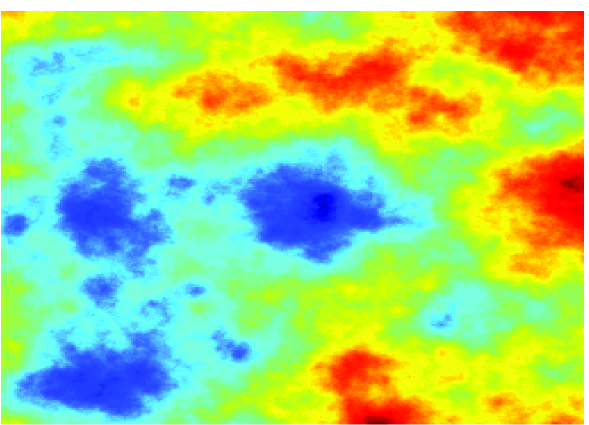
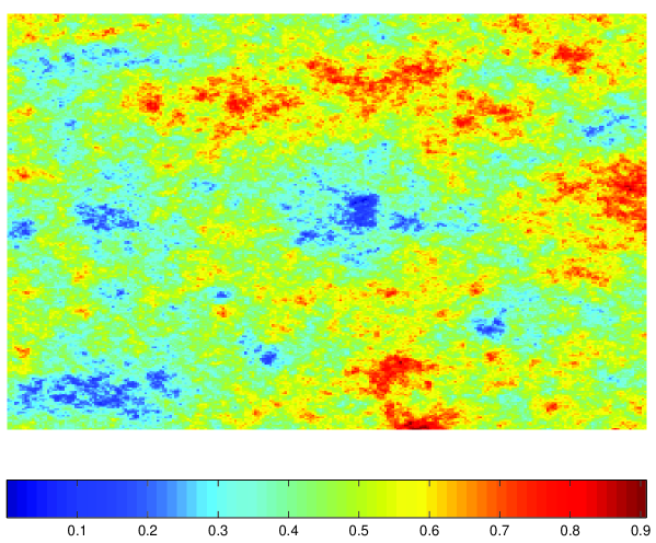
Figure 1: Two different realizations of FBM statistics on a $256\times 256$ square lattice: $H=0.8$ (top) and $H=0.2$ (bottom)

The percolation threshold $p_{c}$ has been defined as the minimum concentration $p$ of filled sites to form an infinite cluster with probability $1$. It has been observed that percolation transitions on long-range self-affine structures behaves differently from ordinary percolation in some important aspects [15]. For example, Marrink et al [16] found that percolation thresholds $p_{c}$ of self-affine lattices are strongly dependent on the spanning rule employed even when the lattice is effectively infinite. Following the work of Reynolds et al [17] on un-correlated square lattices, they considered three different spanning rules for percolation on self-affine models, $\mathcal{R}_{0}$ , the probability of spanning either horizontally or vertically or both, $\mathcal{R}_{1}$, the probability of spanning in a specified direction (e.g. horizontally), and $\mathcal{R}_{2}$, the probability of spanning both horizontally and vertically. The numerical results obtained by Marrink et al established that unlike the urn-correlated random model three critical concentrations: $p_{c}^{eith}$, $p_{c}^{spec}$, and $p_{c}^{both}$ (corresponding to percolation rules $\mathcal{R}_{0}$, $\mathcal{R}_{1}$, and $\mathcal{R}_{2}$ respectively) do not converge for infinite self-affine models. Therefore, the definition of the percolation threshold depends on the desired applications and one must consider the appropriate percolation threshold to obtain critical parameters of percolation transition of self affine models.

At each specified percolation threshold, there exists a distribution of distinct, finite clusters (equilibrium percolation clusters). In this work we made the search for clusters by using the Hoshen-Kopelman algorithm [18]. To remove the effect of boundary conditions from our numerical estimations, we only count those clusters which do not touch lattice boundaries. We call them internal clusters. For each internal cluster of an arbitrary size $s$, we evaluate the cluster radius of gyration tensor G

$$\textbf{G}=\sum_{i=1}^{N}(\overrightarrow{x}_{i}^{2}\textbf{I}-\overrightarrow{x}_{i}\overrightarrow{x}_{i})$$ (4)

In the above definition, $\overrightarrow{x}_{i}$ is the distance of occupied site $i$ from the cluster’s center of mass and $s$ is the size of the cluster. The principal radii of gyration of the cluster, $R_{min}^{2}$ and $R_{max}^{2}$, are obtained via diagonalization of G. At the percolation threshold the variations in the $R^{2}_{i}$, have the following asymptotic form:

$$\langle R^{2}_{i}\rangle=r_{i}s^{2\nu}(1+a_{i}s^{-\theta}+b_{i}s^{-1}+...)\;\;\;\;\;\;\;\;\;\;\;\;i=min\;or\;max$$ (5)

where $\nu$ is the leading scaling exponent and $\theta$ is the non-analytical correction-to-scaling exponent of the cluster. The coefficients $r_{i}$, $a_{i}$, and $b_{i}$ are all independent of $s$ [1]. The shape of the cluster is then characterized by evaluating its anisotropy parameter, as described previously. Finally, we obtain the mean values of anisotropy quantifier by averaging it over all the percolation clusters with the same size $s$, resulted in different lattice realizations. Then, the results have been lumped together at the centers of blocks of size $[2^{m-1},2^{m}]$. This procedure not only helps to eliminate correction-to-scaling for small clusters [4], but it produces new data points which are usually less correlated than the original data [19].

The most time-consuming step in these kind of simulations is generation of FBM statistics itself. Generating FBM on large lattices requires significant CPU time and computer memory. On the other hand, in order to eliminate finite-size effects from numerical results, we need lattices with large $L$ . In this work, we have fixed the linear size of our square lattices to $L=256$ which is both computationally tractable and at the same time large enough to make sure that our results are not affected by finite-size effects [10]. To achieve highly accurate results, we estimate the mean values by sampling a large number of lattice realizations ($30\;000$ samples in each case).

In order to make an appropriate and reliable sampling of cluster shapes in configurations space it is necessary that the medium linear size be large enough such that all possible configurations, including the most anisotropic ones potentially can happen (the condition of effectively infinite large medium). This puts a maximum on cluster size $s$. Indeed, for large clusters , i.e. when $s>>L^{2}$, the condition of effectively infinite large medium would not be fulfilled and as such, the sampling would be in favor of more isotropic configurations.

3 Results

Let us first look at the shape of percolation clusters in completely random media. As mentioned in the first section, the estimated value of $A_{\infty}$ at percolation threshold has been reported by several authors. Here, we provide our estimations of the anisotropy parameters of percolation clusters for some selected values of $p$ in Table1. The total number of lattice realizations has been $100\;000$ in this case. The cluster numbers is a function of $p$, but it always decreases rapidly with $s$ [20]. Therefore, when $|p-p_{c}|$ is not small, the total number of clusters of larger sizes is not large enough to give a reliable statistics and we do not include the anisotropy parameters of such clusters in our reports.

Table 1.The anisotropy parameters of random model

$m$		$p=0.454$		$p=0.550$		$p=0.593$		$p=0.650$
$3$		$.340(4)$		$.355(4)$		$.362(5)$		$.375(6)$
$4$		$.3307(2)$		$.3467(2)$		$.3545(3)$		$.3685(5)$
$5$		$.3319(2)$		$.3511(4)$		$.3607(6)$		$.3786(9)$
$6$		$.3330(1)$		$.3565(3)$		$.3688(4)$		$.3914(7)$
$7$		$.3313(2)$		$.3594(1)$		$.3752(3)$		$.405(1)$
$8$		$.326(1)$		$.3591(1)$		$.3794(2)$		$.419(3)$
$9$		$---$		$.3569(2)$		$.3813(3)$		$---$

As seen from this results, in ordinary percolation the cluster mean anisotropy parameters is a function of both $p$ and $s$. This is natural as the number of a specific cluster configuration in random percolation model is proportional to $p^{s}(1-p)^{t}$, where $s$ is the cluster size and $t$ is its perimeter [20]. In fact more careful investigations show some important trends in the behaviour of $\langle A_{s}(p)\rangle$ as a function of $s$ and $p$. For example, looking at the table we can see that all the values of $s$, the mean anisotropy parameter grows with $p$. Meanwhile, the variation of $\langle A_{s}\rangle$ for a given $p$ is much more complicated. It seems that for $p<p_{c}$, $\langle A_{s}\rangle$ has a maximum at some moderate value of $s$, while when $p>p_{c}$, the larger clusters are always more symmetric than smaller ones. The behaviour of $\langle A_{s}\rangle$ at percolation threshold $p\simeq 0.593$ is consistent with equation2, i.e., it evolves to an asymptotic value at large values of $s$ [1, 2, 3, 4, 5].

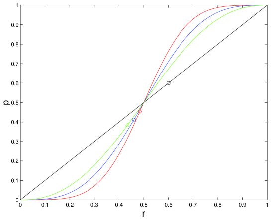
Figure 2: The concentration $p$ of filled sites as a function of cutoff $r$ for random model (black curve), and three different self-affine models: $H=0.2$ (green), $H=0.5$ (blue) and $H=0.8$ (red). In each case, the value of $r^{eith}_{c}$ at $p^{eith}_{c}$ has been marked (circles).

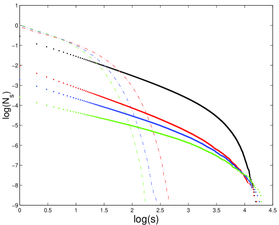
Figure 3: Variation of $N_{s}=\sum_{k\geq s}n_{k}$, where $n_{k}$ is the normalized cluster number of size $k$ for percolation in random model (black) and percolation on either direction in three different self-affine models: $H=0.2$ (green), $H=0.5$ (blue) and $H=0.8$ (red). The dash-dot curves are the $N_{s}$’s in random model when the concentration of filled sites is equal to the $p_{c}^{eith}$ of self affine model when $H=0.2$ (green), $H=0.5$ (blue) and $H=0.8$ (red). In all cases we have only counted the internal percolation clusters of $256\times 256$ square lattices.

To produce the percolation clusters of the self-affine model we have used the percolation thresholds provided in Ref. [16]. In Fig.2 we have shown our estimations of the concentrations $p$ of filled sites as a function of cutoff $r$ for three different values of Hurts exponent, $H=0.2$, $H=0.5$ and $H=0.8$. For random model, $p=r$, but as it is seen this is not the case for self-affine models. In fact, the fraction of occupied sites at both $p_{c}^{eith}$, and $p_{c}^{spec}$ in self-affine models is less than the corresponding values of random model. This is because compared to the random case, the existence of self-affine long-range correlations is in favor of formation of larger clusters. Calculation of $N_{s}=\sum_{k\geq s}n_{k}$, where $n_{k}$ is the total number of clusters with size $k$ per lattice sites (fig.3) for the case of percolation on either direction shows this phenomenon clearly. For comparison, the $N_{s}$’s in random model when the concentration of filled sites is equal to $p_{c}^{eith}$ of self affine models with $H=0.2$, $H=0.5$ and $H=0.8$ are shown too.

Our numerical results for the values of the mean anisotropy parameters at percolation transition in either direction (rule $\mathcal{R}_{0}$) and percolation transition in specified direction (rule $\mathcal{R}_{1}$) have been appeared in fig.4 and fig.5 respectively. For comparison the corresponding values for random percolation have been also included. Interestingly, the differences between these two groups of curves are almost negligible, although the difference between $p_{c}^{eith}$ and $p_{c}^{spec}$ is significant. In fact more investigations suggest that unlike random model, the shape of clusters of the self-affine model do not vary significantly with concentration $p$ of the filled sites. We may conclude that the introduction of isotropic self-affinity subsidizes (and even maybe removes) the dependence of the number of a specific cluster configuration to concentration of filled sites.

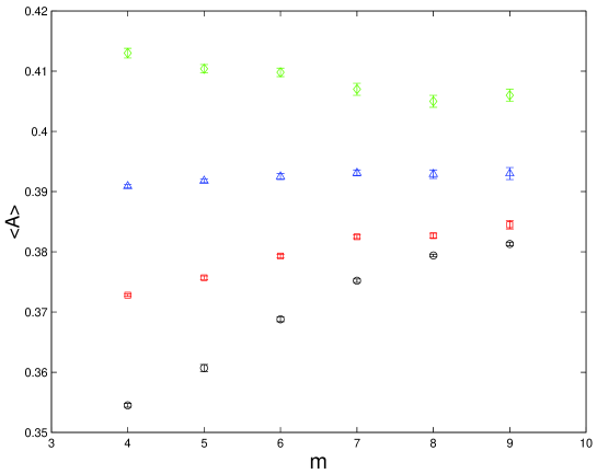
Figure 4: The estimated values of mean anisotropy parameters at $p_{c}^{eith}$ for self-affine models with $H=0.2$ (green), $H=0.5$ (blue) and $H=0.8$ (red). The results have been lumped together at the block centers of size $[2^{m-1},2^{m}]$. For comparison the corresponding values for random percolation at the percolation threshold have been also included (black).

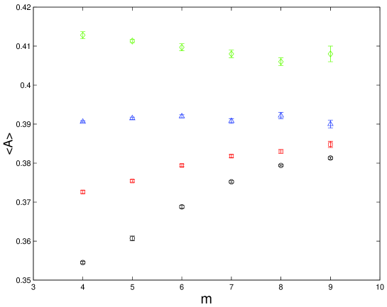
Figure 5: The estimated values of mean anisotropy parameters at $p_{c}^{spec}$ for self affine models with $H=0.2$ (green), $H=0.5$ (blue) and $H=0.8$ (red). The results have been lumped together at the block centers of size $[2^{m-1},2^{m}]$. For comparison the corresponding values for random percolation at the percolation threshold have been also included (black).

One can observe that another important effect of self-affinity is to increase the isotropy of percolation clusters. Meanwhile, the difference between the anisotropy parameters of different $H$’s and random percolation clusters are not significant especially when $H\rightarrow 0$. This result is in agreement with the previous findings which say that in two dimensions, the scaling properties of self-affine model does not differ so much from random model and the difference between the critical exponents of two models vanishes as $H\rightarrow 0$ [10].

While the presence of both kind of long-range correlations increases the isotropy of self affine percolation clusters, there is still a significant qualitative difference between the effect of persistent and anti-persistent correlations on the shape of clusters. Considering the relation:

$$\langle A_{s}\rangle\cong A_{\infty}[1+(a_{min}-a_{max})s^{-\theta}+(b_{\min}-b_{max})s^{-1}]$$ (6)

we can deduce from the behaviour of anisotropy parameters that the sign of correction to scaling term, $(a_{min}-a_{max})s^{-\theta}$, depends on $H$: it is positive for $H<0.5$ and negative for $H>0.5$. At $H=0.5$ this term is almost zero. Hence, for anti-persisting long-range correlations the correction to scaling coefficient $a_{min}$ is larger than $a_{max}$, which means in this case $R^{2}_{min}$ grows faster than $R^{2}_{max}$. Again, we see that anti-persistent self-affine models shows more similarity with random model (see fig.4 or fig.5). In the presence of persisting correlations $R^{2}_{max}$ grows faster than $R^{2}_{min}$ and the anisotropy parameter decreases with $s$. Naturally, for the case $H=0$ which separates these two kinds of correlations, the growth rate of $R^{2}_{min}$ and $R^{2}_{max}$ should be equal.

4 Concluding remarks

We calculated numerically the anisotropy in the shape of equilibrium percolation clusters in long range self-affine correlated square lattices and observed some interesting results. We saw that compared to random percolation, the shape of percolation clusters become slightly more symmetric and the exact value of anisotropy parameter is a function of Hurts exponent. On the other hand, the type of correlations in the medium property, determines the sign of non-analytical correction to scaling contribution into the anisotropy parameters of clusters. In accordance with the previous studies we also observed that the percolation clusters of FBM models become much more similar to those of random models as $H\rightarrow 0$.

Finally, we mention again that, the size of largest cluster that we may consider in our analysis is restricted by the lattice size. To estimate the accurate values of $A_{\infty}$ or non-analytical correction to scaling exponents one should extend the simulation method to larger values of $L$.

The author would like to thank M. Sahimi for useful hints.

References

- [1] Family F and Vicsek T, 1985 Phys. Rev. Lett 55 641.
- [2] Aronovitz J A and Stephen M J, 1987 J. Phys. A: Math. Gen. 20 2539.
- [3] Starley J P and Stephen M J, 1987 J. Phys. A: Math. Gen. 20 6501.
- [4] Quandt S and Young A P, 1987 J. Phys. A: Math. Gen. 20 L851.
- [5] Ebrahimi F, 2008 J. Stat. Mech. P04005
- [6] M.E. Fisher 1967, Physics 3 255 (1967).
- [7] Sahimi M, 1993 Rev. Mod. Phys. 65 1393.
- [8] Hewett T A, 1986 SPE 15836
- [9] Hewett T A and Behrens R A, 1990 SPE Form. Eval. 5 217
- [10] Sahimi M and Mukhopadhyay S, 1996 Phys. Rev. E 54 3870.
- [11] Mandelbrot B B, 1983 The Fractal Geometery of Nature (W. H. Freeman and Company: New York).
- [12] Peitgen H O and Saupe D, 1988 The Science of Fractal Images (Springer-Verlag: New York).
- [13] Mehrabi A R Rassamdana H and Sahimi M, 1997 Phys. Rev. E 56 712.
- [14] Sahimi M, 1994 J. Phys. I 4 1263.
- [15] Schmittbuhl J, Vilotte J P, and Roux S, 1993 J. Phys. A 26 6115
- [16] Marrink S J, Paterson L, and Knacksdtedt M A, 2000 Physica A 280 207
- [17] Reynolds P J, Stanley H E, and Klein W, 1980 Phys. Rev. B 21 1223
- [18] Hoshen J and Kopelman R, 1976 Phys. Rev. B 14 3438
- [19] Flyvbjerg H and Petersen H G, 1989 J. Chem. Phys. 91 461
- [20] Stuffer D and Aharony A, 1995 Introduction to Percolation Theory (Taylor and Francis: London).