Abstract

We study possible crossing of the phantom divide line in a DGP-inspired $F(R,\phi)$ braneworld scenario where scalar field and curvature quintessence are treated in a unified framework. With some specific form of $F(R,\phi)$ and by adopting a suitable ansatz, we show that there are appropriate regions of the parameters space which account for late-time acceleration and admit crossing of the phantom divide line.

Key Words: Braneworld Cosmology, DGP Scenario, Dark Energy Models, Late-time Acceleration
PACS: 04.50.+h,  98.80.-k

1 Introduction

Based on several astronomical evidences, our universe is currently in a period of positively accelerated expansion [1]. It is possible to interpret this late-time acceleration based on yet unknown component called dark energy in literature ( see for instance [2] with a comprehensive list of references therein). Also, it has been shown that such an accelerated expansion could be the result of a modification to the Einstein-Hilbert action ( for a recent review see [3]). On the other hand, DGP braneworld scenario has the capability to interpret this late-time acceleration via leakage of gravity to extra dimension in its self-accelerating branch [4]. For the first alternative, the simplest candidate for dark energy is the cosmological constant itself. However, it suffers from serious problems such as a huge amount of fine-tuning [2,5,6]. Within dark energy viewpoint, for a dark energy component, say $X$, its equation of state or equivalently equation of state parameter $\omega_{X}=\frac{p_{X}}{\rho_{X}}$, determines both gravitational properties and evolution of the dark energy. Recent constraints on equation of state of dark energy indicate that $p_{X}\approx-\rho_{X}$ and even that $\omega_{X}<-1$. When we consider background evolution, there is no problem with $\omega_{X}<-1$. However, there will be apparent divergencies in perturbation when one crosses the phantom divide line, $\omega_{X}=-1$. Accordingly, crossing of the phantom divide line, $\omega_{X}=-1$, provides a suitable basis to test alternative theories of gravity or higher dimensional models which can give rise to an effective phantom energy [6]. With these motivations, the issue of phantom divide line crossing has been investigated extensively in recent years ( see [6] and references therein). In principle, crossing of phantom divide line by the dark energy equation of state parameter at recent red-shifts, has two possible cosmological implications: either the dark energy consists of multiple components with at least one non-canonical phantom component or general relativity needs to be extended to a more general theory on cosmological scales. Both of these conjectures have been studied extensively. For instance, curvature quintessence [7] is a fascinating proposal in this respect. Recently, phantom-like behavior in a brane-world model with curvature effects and also in dilatonic brane-world scenario with induced gravity have been reported [8]. Dark energy models with non-minimally coupled scalar field and other extensions of scalar-tensor theories have been studied widely some of which can be found in reference [9]. In the spirit of scalar-tensor dark energy models, our motivation here is to show that a general $F(R,\phi)$   DGP-inspired scenario can account for late-time acceleration and crossing of phantom divide line in some suitable domains of model parameters space. To show this feature, first we study cosmological dynamics of $F(R,\phi)$  DGP-inspired scenario briefly. In the minimal case, motivated by modified theories of gravity, some authors have included a term of the type $\ell_{0}R^{n}$ in the action [7,10]. This extension for some values of $n$ has the capability to explain late-time acceleration of the universe in a simple manner. It is then natural to extend this scenario to more general embedding of DGP inspired scenarios. The purpose of this paper is to perform such a generalization to study both late-time acceleration and possible crossing of phantom divide line in this setup. We focus mainly on the potential of the type $V(\phi)=\lambda\phi^{\eta}$ for non-minimally coupled scalar field. Our setup for minimal case predicts a power-law acceleration supporting observed late-time acceleration. In the non-minimal case, by a suitable choice of non-minimal coupling and scalar field potential, one obtains accelerated expansion in some specific regions of parameters space. While a single minimally coupled scalar field in four dimensions cannot reproduce a crossing of the phantom divide line for any scalar field potential [11], a non-minimally coupled scalar field account for such a crossing [6]. In DGP model, equation of state parameter of dark energy never crosses $\omega(z)=-1$ line, and universe eventually turns out to be de Sitter phase. Nevertheless, in this setup if we include a single scalar field (ordinary or phantom) on the brane, we can show that equation of state parameter of dark energy can cross phantom divide line [12]. Crossing of phantom divide line with non-minimally coupled scalar field on the warped DGP brane has been studied recently [13]. Our purpose here is to obtain an extension of these non-minimal dark energy models within DGP-inspired $F(R,\phi)$ braneworld scenario. We use a prime for differentiation with respect to $R$. An overdot marks differentiation with respect to the brane time coordinate.

2 $F(R,\phi)$ DGP-Inspired Gravity

We start with the following action

$$S=\frac{m_{4}^{3}}{2}\int d^{5}(x)\sqrt{-g}\Re+\int d^{4}(x)\sqrt{-q}\Big{(}\frac{m_{3}^{2}}{2}F(R,\phi)-\frac{1}{2}q^{\mu\nu}\nabla_{\mu}\phi\nabla_{\nu}\phi-V(\phi)+m_{4}^{3}\overline{K}+L_{m}\Big{)},$$ (1)

where the first term shows the usual Einstein-Hilbert action in 5D bulk with 5D metric denoted by $g_{AB}$ and Ricci scalar denoted by $\Re$. The second term on the right is a generalization of the Einstein-Hilbert action induced on the brane. This is an extension of the scalar-tensor theories in one side and a generalization of $f(R)$-gravity on the other side. We call this model as $F(R,\phi)$  DGP-inspired scenario. $y$ is the coordinate of the fifth dimension and we suppose that brane is located at $y=0$ . $q_{\mu\nu}$ is induced metric on the brane which is connected to $g_{AB}$ via $q_{\mu\nu}=\delta_{\mu}\,^{A}\delta_{\nu}\,^{B}g_{AB}$. $\overline{K}$  is the trace of the mean extrinsic curvature of the brane defined as follows

$$\overline{K}_{\mu\nu}=\frac{1}{2}\lim_{\epsilon\longrightarrow+0}\bigg{(}[K_{\mu\nu}]_{y=-\epsilon}+[K_{\mu\nu}]_{y=+\epsilon}\bigg{)}$$ (2)

We denote matter field Lagrangian by $L_{m}(q_{\mu\nu},\psi)$ with the following energy-momentum tensor

$$T_{\mu\nu}=-2\frac{\delta L_{m}}{\delta q^{\mu\nu}}+q^{\mu\nu}L_{m}.$$ (3)

The pure scalar field lagrangian is $L_{\phi}=\frac{1}{2}q^{\mu\nu}\nabla_{\mu}\phi\nabla_{\nu}\phi-V(\phi)$ which gives the following energy-momentum tensor

$$\top_{\mu\nu}=\nabla_{\mu}{\phi}\nabla_{\nu}\phi-\frac{1}{2}q_{\mu\nu}(\nabla\phi)^{2}-q_{\mu\nu}V(\phi)$$ (4)

The field equations resulting from this action are given as follows

$$\frac{m_{4}^{3}}{F^{\prime}(R,\phi)}\bigg{(}\Re_{AB}-\frac{1}{2}g_{AB}\Re\bigg{)}+m_{3}^{2}\delta_{A}\,^{\mu}\delta_{B}\,^{\nu}\Big{(}R_{\mu\nu}-\frac{1}{2}q_{\mu\nu}R\Big{)}\delta(y)=\delta_{A}\,^{\mu}\delta_{B}\,^{\nu}(\hat{T}_{\mu\nu}+\hat{\top}_{\mu\nu}+T_{\mu\nu}^{curv})\delta(y).$$ (5)

In this relation $\hat{T}_{\mu\nu}=\frac{T_{\mu\nu}}{F^{\prime}(R,\phi)}$ where $T_{\mu\nu}$ is the energy-momentum tensor in matter frame and $\hat{\top}_{\mu\nu}=\frac{\top_{\mu\nu}}{F^{\prime}(R,\phi)}$. Also, $T_{\mu\nu}^{curv}$ is defined as follows

$$T_{\mu\nu}^{curv}=\frac{m_{3}^{2}}{F^{\prime}(R,\phi)}\bigg{[}\frac{1}{2}q_{\mu\nu}\bigg{(}F(R,\phi)-RF^{\prime}(R,\phi)\bigg{)}+\bigg{(}F^{\prime}(R,\phi)\bigg{)}^{;\alpha\beta}\bigg{(}q_{\mu\alpha}q_{\nu\beta}-q_{\mu\nu}q_{\alpha\beta}\bigg{)}\bigg{]}.$$ (6)

In the bulk, $T_{AB}=0$ and therefore

$$G_{AB}=\Re_{AB}-\frac{1}{2}g_{AB}\Re=0$$ (7)

and on the brane we have

$$G_{\mu\nu}=R_{\mu\nu}-\frac{1}{2}q_{\mu\nu}R=\frac{\tau_{\mu\nu}}{m_{3}^{2}},$$ (8)

where $\tau_{\mu\nu}=\hat{T}_{\mu\nu}+\hat{\top}_{\mu\nu}+T_{\mu\nu}^{curv}$. The corresponding junction conditions relating quantities on the brane are as follows

$$\lim_{\epsilon\longrightarrow+0}[K_{\mu\nu}]_{y=-\epsilon}^{y=+\epsilon}=\frac{F^{\prime}(R,\phi)}{m_{4}^{3}}\bigg{[}\tau_{\mu\nu}-\frac{1}{3}q_{\mu\nu}q^{\alpha\beta}\tau_{\alpha\beta}\bigg{]}_{y=0}-$$

$$\frac{m_{3}^{2}}{m_{4}^{3}}F^{\prime}(R,\phi)\bigg{[}R_{\mu\nu}-\frac{1}{6}q_{\mu\nu}q^{\alpha\beta}R_{\alpha\beta}\bigg{]}_{y=0}$$ (9)

A detailed study of weak field limit of this scenario within harmonic gauge on the longitudinal coordinates and using Green’s method to find gravitational potential, leads us to a modified (effective) cross-over distance in this set-up as follows ( see [14] for details of a similar argument)

$$\ell_{F}=\frac{m_{3}^{2}}{2m_{4}^{3}}\bigg{(}\frac{dF}{dR}\bigg{)}=\bigg{(}\frac{dF}{dR}\bigg{)}\ell_{DGP},$$ (10)

where $\ell_{DGP}=\frac{m_{3}^{2}}{2m_{4}^{3}}.$ The gravitational potential in this scenario takes the following forms in two different extreme:
For  $r\ll\ell_{F}$

$$U(r)=-\frac{(M_{\psi}+M_{\phi})}{6\pi m_{3}^{2}F^{\prime}(R,\phi)r}\bigg{[}1+(\gamma-\frac{2}{\pi})\frac{r}{\ell_{F}}+\frac{r}{\ell_{F}}\ln(\frac{r}{\ell_{F}})+O(\frac{r^{2}}{\ell_{F}^{2}})\bigg{]}$$ (11)

and for  $r\gg\ell_{F}$

$$U(r)=-\frac{(M_{\psi}+M_{\phi})}{6\pi^{2}m_{4}^{3}r^{2}}\bigg{[}1-\frac{2\ell_{F}^{2}}{r^{2}}+O(\frac{\ell_{F}^{4}}{r^{4}})\bigg{]}.$$ (12)

$M_{\phi}$ is effective mass of the scalar field $\phi$ which is non-minimally coupled to induced gravity, $M_{\psi}$ collectively shows the effective mass of other material fields minimally coupled to gravity and $\gamma=0.577$ is Euler’s constant. The most important feature of this $F(R,\phi)$  DGP-inspired scenario is the fact that now cross-over scale is explicitly related to the induced curvature on the brane and non-minimal coupling of scalar field with this curvature. Since the dynamics of scalar field $\phi$ is described by $\nabla^{\mu}\phi\nabla_{\mu}\phi-\frac{dV}{d\phi}+\frac{m_{3}^{2}}{2}\frac{dF}{d\phi}=0$, one may explain this result as a spacetime variation of the Newton’s constant. In this viewpoint, when $F(R,\phi)$ varies from point to point on DGP brane, the crossover scale takes different values. Recent best-fit crossover scale is given by  $\ell_{DGP}=1.26H_{0}^{-1}$  [15] where  $H_{0}^{-1}\sim 3000Mpc$. Since $\frac{dF}{dR}=\frac{2m_{4}^{3}\ell_{F}}{m_{3}^{2}}$, if we choose  $\ell_{F}\sim 1.26H_{0}^{-1}$  it is possible to constraint this $F(R,\phi)$ scenario to be consistent with observational data. For instance, if we set $F(R,\phi)=\alpha(\phi)R$ it is easy to show that $\alpha(\phi)$ can attain the value of $\alpha(\phi)\sim 2.52\times 10^{-30}H_{0}^{-1}$ where we have assumed  $m_{4}\sim 10^{3}GeV$ and $m_{3}\sim 10^{18}GeV$. This argument has the potential to be used as a mechanism for obtaining reliable form of $F(R,\phi)$ in cosmological context.

3 Cosmological Implications of the Model

Embedding of FRW cosmology in DGP scenario (which deviates from general relativity at large distances) is possible in the sense that this model accounts for cosmological equations of motion at any distance scale on brane with any function of Ricci scalar. It is well-known that original DGP model explains late-time acceleration via leakage of gravity to extra dimension. On the other hand, in this model equation of state parameter of dark energy never crosses the phantom divide line. Extension of DGP scenario to more generalization of the brane action may result in several new implications on cosmological ground. In this respect, it is interesting to know whether DGP-inspired $F(R,\phi)$ gravity can account for late-time acceleration and especially phantom divide line crossing. With this motivation, in this section we investigate cosmological implications of our setup focusing firstly on the late-time acceleration. We assume the following line element

$$ds^{2}=q_{\mu\nu}dx^{\mu}dx^{\nu}+b^{2}(y,t)dy^{2}=-n^{2}(y,t)dt^{2}+a^{2}(y,t)\gamma_{ij}dx^{i}dx^{j}+b^{2}(y,t)dy^{2}$$ (13)

where $\gamma_{ij}$ is a maximally symmetric 3-dimensional metric defined as $\gamma_{ij}=\delta_{ij}+k\frac{x_{i}x_{j}}{1-kr^{2}}$ where  $k=-1,0,1$   parameterizes the spatial curvature and $r^{2}=x_{i}x^{i}$. We assume that the scalar field $\phi$ depends only on the cosmic time of the brane. Choosing a Gaussian normal coordinate system so that $b^{2}(y,t)=1$, non-vanishing components of Einstein’s tensor in the bulk plus junction conditions on the brane defined as

$$\lim_{\epsilon\longrightarrow+0}[\partial_{y}n]_{y=-\epsilon}^{y=+\epsilon}(t)=\frac{2nm_{3}^{2}}{m_{4}^{3}}\bigg{[}\Big{(}\frac{dF}{dR}\Big{)}\Big{(}\frac{\ddot{a}}{n^{2}a}-\frac{\dot{a}^{2}}{2n^{2}a^{2}}-\frac{\dot{n}\dot{a}}{n^{3}a}-\frac{k}{2a^{2}}\Big{)}\bigg{]}_{y=0}$$

$$+\frac{n}{3m_{4}^{3}}\bigg{[}\Big{(}\frac{dF}{dR}\Big{)}\Big{(}2\rho^{(tot)}+3p^{(tot)}\Big{)}\bigg{]}_{y=0},$$ (14)

$$\lim_{\epsilon\longrightarrow+0}[\partial_{y}a]_{y=-\epsilon}^{y=+\epsilon}(t)=\frac{m_{3}^{2}}{m_{4}^{3}}\bigg{[}\Big{(}\frac{dF}{dR}\Big{)}\Big{(}\frac{\dot{a}^{2}}{n^{2}a}+\frac{k}{a}\Big{)}\bigg{]}_{y=0}-\bigg{[}\bigg{(}\frac{dF}{dR}\bigg{)}\frac{\rho^{(tot)}a}{3m_{4}^{3}}\bigg{]}_{y=0}$$ (15)

yield the following generalization of Friedmann equation for cosmological dynamics on the brane ( see [14] for machinery of calculations for a simple case)

$$H^{2}+\frac{k}{a^{2}}=\frac{1}{3m_{3}^{2}F^{\prime}(R,\phi)}\Bigg{(}\rho^{tot}+\rho_{0}\bigg{[}1+\epsilon\sqrt{1+\frac{2}{\rho_{0}}\bigg{[}\rho^{tot}-\frac{m_{3}^{2}F^{\prime}(R,\phi)\varepsilon_{0}}{a^{4}}\bigg{]}}\bigg{]}\Bigg{)}$$ (16)

where $\epsilon=\pm 1$ shows two different embedding of the brane,   $\rho_{0}=\frac{6m_{4}^{6}}{m_{3}^{2}F^{\prime}(R,\phi)}$  and  $\varepsilon_{0}=3\Big{(}\frac{\dot{a}^{2}}{n^{2}}-a^{\prime 2}+k\Big{)}a^{2}$  is a constant ( with $a^{\prime}\equiv\frac{da}{dy}$). Total energy density and pressure are defined as  $\rho^{(tot)}=\hat{\rho}+\rho_{\phi}+\rho^{curv}$,  $p^{(tot)}=\hat{p}+p_{\phi}+p^{curv}$  respectively. The ordinary matter on the brane has a perfect fluid form with energy density $\hat{\rho}$ and pressure $\hat{p}$, while the energy density and pressure corresponding to non-minimally coupled scalar field and also those related to curvature are given as follows

$$\rho_{\varphi}=\bigg{[}\frac{1}{2}\dot{\phi}^{2}+n^{2}V(\phi)-6\frac{dF}{d\phi}H\dot{\phi}\bigg{]}_{y=0},$$ (17)

$$p_{\phi}=\bigg{[}\frac{1}{2n^{2}}\dot{\phi}^{2}-V(\phi)+\frac{2}{n^{2}}\frac{dF}{d\phi}(\ddot{\phi}-\frac{\dot{n}}{n}\dot{\phi})+4\frac{dF}{d\phi}\frac{H}{n^{2}}\dot{\phi}+\frac{2}{n^{2}}\frac{d^{2}F}{d\phi^{2}}\dot{\phi}^{2}\bigg{]}_{y=0}.$$ (18)

also

$$\rho^{curv}=\frac{m_{3}^{2}}{F^{\prime}(R,\phi)}\bigg{(}\frac{1}{2}\bigg{[}F(R,\phi)-RF^{\prime}(R,\phi)\bigg{]}-3\dot{R}HF^{\prime\prime}(R,\phi)\bigg{)},$$ (19)

$$p^{curv}=\frac{m_{3}^{2}}{F^{\prime}(R,\phi)}\bigg{(}{2\dot{R}HF^{\prime\prime}(R,\phi)+\ddot{R}F^{\prime\prime}(R,\phi)+\dot{R}^{2}F^{\prime\prime\prime}(R,\phi)-\frac{1}{2}\Big{[}F(R,\phi)-RF^{\prime}(R,\phi)\Big{]}}\bigg{)}.$$ (20)

where $H=\frac{\dot{a}(0,t)}{a(0,t)}$  is the Hubble parameter. Ricci scalar on the brane is given by

$$R=3\frac{k}{a^{2}}+\frac{1}{n^{2}}\bigg{[}6\frac{\ddot{a}}{a}+6\Big{(}\frac{\dot{a}}{a}\Big{)}^{2}-6\frac{\dot{a}}{a}\frac{\dot{n}}{n}\bigg{]}.$$

In this setup, non-minimal coupling of scalar field and induced gravity leads to no-conservation of effective energy density on the brane

$$\dot{\rho}^{(tot)}+3H\Big{(}\rho^{(tot)}+p^{(tot)}\Big{)}=6\Big{(}\frac{dF}{d\phi}\Big{)}\dot{\phi}(H^{2}+\frac{k}{a^{2}}).$$ (21)

It is easy to show that for a minimally coupled scalar field on the brane, this setup yields a late-time accelerating universe in a fascinating manner [10]. The evolution of the scalar field on the brane for a spatially flat FRW geometry, $(k=0)$, is described by the following equations

$$H^{2}=\frac{1}{3m_{3}^{2}F^{\prime}(R,\phi)}\rho^{(tot)}$$ (22)

and

$$\ddot{\phi}+3H\dot{\phi}+\frac{dV(\phi)}{d\phi}=\frac{dF(R,\phi)}{d\phi}.$$ (23)

and finally

$$\frac{\ddot{a}(0,t)}{a(0,t)}=-\frac{1}{6m_{3}^{2}F^{\prime}(R,\phi)}\bigg{[}\rho^{tot}+3p^{tot}\bigg{]}.$$ (24)

These equations show that essentially embedding of FRW cosmology in DGP setup is possible. Now, after a brief study of gravitational and cosmological implications of our setup, we investigate late-time acceleration and crossing of the phantom divide line in this setup.

3.1 Accelerated Expansion

Standard DGP model itself has the capability to explain the late-time acceleration of the universe via leakage of gravity to extra dimensions without any additional mechanism [4]. In our $F(R,\phi)$ DGP inspired model, it is interesting to see whether there is any room for explanation of this late time acceleration. The viability of this question lies in the fact that generally with non-minimal coupling it is harder to achieve accelerated expansion [16]. We first obtain a necessary condition for the acceleration of the universe in $F(R,\phi)$ DGP-inspired model. Then we use a simple ansatz to clarify our general equations. Suppose that scalar field is the only source of matter on the brane so that $\hat{\rho}=0$ for other matter candidates. The necessary condition for acceleration of the universe is  $(\rho_{\phi}+\rho^{curv})+3(p_{\phi}+p^{curv})<0$ because in our $F(R,\phi)$ setup scalar field and curvature are correlated. Therefore we obtain

$$2\bigg{(}1+3\frac{d^{2}F}{d\phi^{2}}\bigg{)}\dot{\phi}^{2}+6\Big{(}\frac{dF}{d\phi}\Big{)}\Big{(}H\dot{\phi}+\ddot{\phi}\Big{)}+\frac{3m_{3}^{2}}{F^{\prime}(R,\phi)}\bigg{[}\dot{R}^{2}F^{\prime\prime\prime}(R,\phi)+F^{\prime\prime}(R,\phi)\Big{(}\dot{R}H+\ddot{R}\Big{)}\bigg{]}-$$

$$m_{3}^{2}\bigg{(}\frac{F(R,\phi)}{F^{\prime}(R,\phi)}-R\bigg{)}-2V(\phi)<0.$$

Using the Klein-Gordon equation (23), this relation can be rewritten as follows

$$2\bigg{(}1+3\frac{d^{2}F}{d\phi^{2}}\bigg{)}\dot{\phi}^{2}+6\Big{(}\frac{dF}{d\phi}\Big{)}^{2}-6\Big{(}\frac{dF}{d\phi}\Big{)}\Big{(}2H\dot{\phi}+\frac{dV}{d\phi}\Big{)}+\frac{3m_{3}^{2}}{F^{\prime}(R,\phi)}\bigg{[}\dot{R}^{2}F^{\prime\prime\prime}(R,\phi)+F^{\prime\prime}(R,\phi)\Big{(}\dot{R}H+\ddot{R}\Big{)}\bigg{]}-$$

$$m_{3}^{2}\bigg{(}\frac{F(R,\phi)}{F^{\prime}(R,\phi)}-R\bigg{)}-2V(\phi)<0.$$ (25)

This is a general condition for acceleration of the universe in our $F(R,\phi)$ DGP inspired model. It is a complicated relation and one cannot achieve an explicit intuition of acceleration in this setup. For simple forms of $F(R,\phi)$ we can find relatively simple conditions that can be explained more explicitly. As a simple example and following Faraoni [16], if we set  $F(R,\phi)=\frac{1}{2}(1-\xi\phi^{2})R$ which gives conformal coupling of scalar field and Einstein gravity, equation (25) under assumption of weak energy condition $\rho_{\phi}\geq 0$, gives $V-\frac{3\xi}{2}\phi\frac{dV}{d\phi}>0$, where we have assumed $\xi\leq\frac{1}{6}$ [16]. For instance, if we set $V(\phi)=\lambda\phi^{\eta}$, we find $\eta<\frac{2}{3\xi}$. Using the ansatz $a(t)\approx At^{\nu}$ and $\phi(t)\approx Bt^{-\mu}$, equations (22) and (23) with  $F(R,\phi)=\frac{1}{2}(1-\xi\phi^{2})R$ and $\hat{\rho}=0$, give $\xi\geq\frac{1}{12}$ with positive and real $\nu$ and considering terms of order  ${\it O}(t^{-\mu-2})$. In this case  $\xi$ is restricted to the interval  $\frac{1}{12}\leq\xi\leq\frac{1}{6}$ and since equation (23) with these ansatz gives $\mu^{2}+(1-3\nu)\mu+12\xi\nu^{2}+6\xi\nu=0$, positivity and reality of solutions for $\mu$ gives $(9-48\xi)\nu^{2}-(6-24\xi)\nu+1\geq 0$. For $\xi=\frac{1}{12}$, we find $\nu=(4\pm\sqrt{11})/5$ which gives a power-law accelerated expansion for positive sign. Therefore, a suitable fine-tuning of non-minimal coupling provides the possibility of late-time accelerated expansion. Based on a dark energy model, to have an accelerated universe, the value of conformal NMC should be restricted to the interval  $0.146\leq\xi\leq 0.167$ [17]. On the other hand, current experimental limits on the time variation of $G$ constraint the nonminimal coupling as $-10^{-2}\preceq\xi\preceq 10^{-2}$ [18]. Solar system experiments such as Shapiro time delay and deflection of light have constraint Brans-Dike parameter to be $\omega_{BD}>500$ which leads to the result of $|\xi|\preceq 2.2\times 10^{-2}$ for non-minimal coupling [18]. However, other approaches lead to different constraints on the value of conformal coupling [19]. As a second and more general example with $R^{n}$ correction, we set  $F(R,\phi)=\frac{1}{2}(1-\xi\phi^{2})\ell_{0}R^{n}$. For spatially flat FRW geometry the Ricci scalar is given by

$$R=6\frac{\ddot{a}}{a}+6\Big{(}\frac{\dot{a}}{a}\Big{)}^{2}.$$ (26)

Using the above proposed ansatz for $a(t)$ and $\phi(t)$, equations (22) and (24) can be rewritten as the following explicit time-dependent form

$$3m_{3}^{2}\nu^{2}\ell_{0}n(12\nu^{2}-6\nu)^{n-1}\Big{(}1-\xi B^{2}t^{-2\mu}\Big{)}=$$

$$B^{2}\mu^{2}t^{-2\mu+2n-2}+2\lambda B^{\eta}t^{-\mu\eta+2n}-12\xi\nu\mu B^{2}\ell_{0}(12\nu^{2}-6\nu)^{n}t^{-2\mu-2}+m_{3}^{2}t^{2n-2}\Big{(}(12\nu^{2}-6\nu)(\frac{1}{n}-1)+6\nu(n-1)\Big{)}$$ (27)

$$-3m_{3}^{2}\nu(\nu-1)\ell_{0}n(12\nu^{2}-6\nu)^{n-1}t^{-2n+2}\Big{(}1-\xi B^{2}t^{-2\mu}\Big{)}=$$

$$2B^{2}\mu^{2}t^{-2\mu}-6\xi B^{2}\mu\ell_{0}(12\nu^{2}-6\nu)^{n}t^{-2n-2\mu}\Big{(}\mu+2\nu\Big{)}+6\xi\ell_{0}(12\nu^{2}-6\nu)^{n}t^{-2n+2}\Big{(}\xi B^{2}\ell_{0}(12\nu^{2}-6\nu)^{n}t^{-2n-2\mu}$$

$$+\lambda\eta B^{\eta}t^{-\mu\eta}\Big{)}+2\lambda B^{\eta}t^{-\mu\eta+2}+6m_{3}^{2}(n-1)(2n-\nu-1)-m_{3}^{2}(\frac{1}{n}-1)(12\nu^{2}-6\nu).$$ (28)

Our aim is to see whether these equations account for positively accelerated expansion with suitable values of parameters. Since the parameter space of the problem is complicated, analytical solutions of these equations have no obvious interpretation. Therefore, we try to see how a suitable choice of parameters leads to viability of accelerated expansion in this setup. Our strategy is to see how with different choices of parameters in equations (27) and (28), equality in this equations is preserved. Firstly, we choose $\nu>1$ in the favor of late-time positively accelerated expansion. We find appropriate values of other parameters in this parameters space as shown in table $1$ and $2$. We plot each side of equation (27) as a separate function of time for some values of parameters. Existence of intersection point for these functions shows the viability of values attributed to parameters to preserve equality. The same procedure for both sides of equation (28) is done too. In summary, to have accelerated expansion, we need $\nu>1$, so choosing $\nu>1$ we find some possible values of the other parameters to have at least one intersection point in the graph and therefore to be consistent with accelerated expansion. Secondly, choosing some specific values for other parameters, we obtain possible values of $\nu$. If there is no intersection between two graphs, it means that with that choice of parameters we will not arrive at $\nu>1$ corresponding to accelerated expansion. If there is intersection but with $\nu<1$, the solution will be decelerating ruled out by observational data. The results of these analysis are shown in table $1$ and $2$ and also in figures $1$, $2$, $3$ and $4$. Note that these are only some specific examples and the actual parameter space is very large and complicate. However, the least advantage of this analysis is the fact that essentially late-time acceleration can be explained naturally within our setup. We see for instance that with $\eta=4$, $n=1.4$, and $\xi=0.166$ there is no possibility to have accelerated expansion with $\nu=1.2$  since there is no intersection point in the graph. On the other hand, accelerated expansion with $\nu=2$ requires $\eta=2$ or $\eta=4$, $n=1.5$, and $\xi=-0.166$ for instance. As a common role in this analysis, we have noticed that from equation (27), only for positive values of $n$ with $1.37\leq n<2$ and for positive or negative $\xi$ there are intersection points and therefore accelerated expansion. These analysis, though very simple and especial, show that $F(R,\phi)$ DGP-inspired scenarios essentially account for positively accelerated expansion.

Table 1: Some choices of parameters for equation (27) to be preserved. The last column shows the coordinate of intersection points and equality of two sides of equation (27) with corresponding choices of parameters.

$\eta$	$n$	$\nu$	$\xi$	$(a,b)$
$2$	$1.4$	$1.2$	$-0.166$	$(1.4,16.4),(7.6,15.2)$
$2$	$1.4$	$1.2$	$0.166$	$(7.6,15.2)$
$4$	$1.4$	$1.2$	$-0.166$	$(1.4,16.5)$
$4$	$1.4$	$1.2$	$0.166$	$--$
$2$	$1.5$	$2$	$-0.166$	$(1.6,114)$
$2$	$1.5$	$2$	$0.166$	$--$
$4$	$1.5$	$2$	$-0.166$	$(1.6,114)$
$4$	$1.5$	$2$	$0.166$	$--$

Table 2: Some choices of parameters for equation (28) to be preserved. The last column shows the coordinate of intersection points and equality of two sides of equation (28) with corresponding choice of parameters. Note that these are only some example and the actual parameter space is very wide.

$\eta$	$n$	$\nu$	$\xi$	$(a,b)$
$2$	$-0.37$	$1.005$	$-0.166$	$(63.4,46.4)$
$2$	$-0.37$	$1.005$	$0.166$	$(122,281)$
$4$	$-0.37$	$1.005$	$-0.166$	$(92.4,128)$
$4$	$-0.37$	$1.005$	$0.166$	$(92.4,128)$
$2$	$-0.5$	$1.2$	$-0.166$	$(16.9,52)$
$2$	$-0.5$	$1.2$	$0.166$	$(20.6,96.3)$
$4$	$-0.5$	$1.2$	$-0.166$	$(19,69.4)$
$4$	$-0.5$	$1.2$	$0.166$	$(19,69.4)$

Note that in minimal case where $F(R,\phi)\propto R^{n}$ one finds from (22) and (24) [20]

$$\nu[\nu(n-2)+(n-1)(2n-1)]=0$$ (29)

$$\nu[\nu(n-2)+n^{2}-n+1]=n(2n-1)(n-1)$$ (30)

from which the allowed solutions are

$$\nu=0\Rightarrow n=0,\,\,\,n=\frac{1}{2},\,\,\,n=1$$

$$\nu=\frac{(n-1)(2n-1)}{(2-n)},\,for\,all~{}n~{}except~{}n=2$$ (31)

Our choices of parameters in preceding discussions are based on this argument and also constraints on non-minimal coupling from reference [19]. Especially, we have taken into account the following considerations: the solutions with $\nu=0$ are not interesting at all since they provide static cosmologies with non-evolving scale factor on the brane. In ordinary 4D gravity with the action of the form $F(R)=\ell_{0}R^{n}$ and without any matter, a constant scale factor with a singular equation of state is achieved for $n=1$. Similarly, in the normal DGP model, that is, when $n=1$ and with no ordinary matter present, we cannot define the equation of state because the scale factor on the brane is constant and equation of state parameter will be singular [10,20]. In our $F(R,\phi)$ setup with  $F(R,\phi)=\frac{1}{2}(1-\xi\phi^{2})\ell_{0}R^{n}$, as we have discussed previously, to have accelerated expansion we need to rstrict $n$ to the interval $1.37\leq n<2$. In this situation, there is no term with the first power of the Ricci scalar to obtain ordinary Einstein-like interactions between two astrophysical objects, such as the Sun and Mercury. To overcome this problem in our setup, we have treated the case with $n=1$ separately after equation (25) above. On the other hand, if we choose theories such as $F(R,\phi)=\frac{1}{2}(1-\xi\phi^{2})\Big{[}R-(1-n)\zeta^{2}\Big{(}\frac{R}{\zeta^{2}}\Big{)}^{n}\Big{]}$ where $\zeta$ is a suitably chosen parameter, our model will contain the case with $n=1$ and therefore general relativity. We will come back to this issue later with more details.

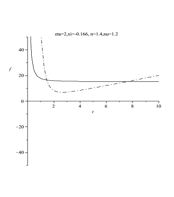
Figure 1: Choosing $\eta=2$, $\xi=-0.166$ and $n=1.4$, we find $\nu=1.2$ from equation (27). There are two intersection points accounting for positively accelerated expansion within $F(R,\phi)=\frac{1}{2}(1-\xi\phi^{2})\ell_{0}R^{n}$ scenario.

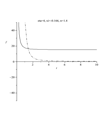
Figure 2: Choosing $\eta=4$, $\xi=-0.166$ and $n=1.4$, we find $\nu=1.2$ from equation (27). There is one intersection point accounting for equality of two sides of equation (27) and positively accelerated expansion with this choice of parameters.

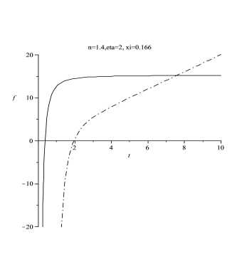
Figure 3: Choosing $\eta=2$, $\xi=+0.166$ ( a positive non-minimal coupling) and $n=1.4$, we find $\nu=1.2$ from equation (28). There is one intersection point accounting for equality of two sides of equation (28) and positively accelerated expansion with this choice of parameters.

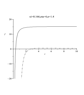
Figure 4: Choosing $\eta=4$, $\xi=+0.166$ and $n=1.4$. In this case there is no intersection point between two sides of equation (27) corresponding to $\nu=1.2$. It is interesting to note that even with other values of $\nu>1$, there is no intersection point. Therefore, it is impossible to have accelerated expansion in this case.

4 Dynamics of Equation of state Parameter

Because of explicit interaction between scalar field and curvature, the equation of state parameter for non-minimally coupled scalar field in this $F(R,\phi)$  DGP-inspired setup is as follows

$$\omega=\frac{P^{(tot)}}{\rho^{(tot)}}=\frac{P^{(curv)}+P_{\phi}}{\rho^{(curv)}+\rho_{\phi}}.$$ (32)

which can be written as

$$\omega=\frac{\big{(}\frac{1}{2}+2\frac{d^{2}F}{d\phi^{2}}\big{)}\dot{\phi}^{2}-V(\phi)+2\frac{dF}{d\phi}\big{(}\ddot{\phi}+2H\dot{\phi}\big{)}+\frac{m_{3}^{2}}{F^{\prime}(R,\phi)}\big{[}\big{(}2\dot{R}H+\ddot{R}\big{)}F^{\prime\prime}(R,\phi)+\dot{R}^{2}F^{\prime\prime\prime}(R,\phi)-\frac{1}{2}F(R,\phi)+\frac{1}{2}RF^{\prime}(R,\phi)\big{]}}{\frac{1}{2}\dot{\phi}^{2}+V(\phi)-6\frac{dF}{d\phi}H\dot{\phi}+\frac{m_{3}^{2}}{F^{\prime}(R,\phi)}\big{(}\frac{1}{2}F(R,\phi)-\frac{1}{2}RF^{\prime}(R,\phi)-3\dot{R}H\frac{d^{2}F}{dR^{2}}\big{)}},$$ (33)

This is a general statement for equation of state in $F(R,\phi)$ setup. To proceed further, we have to specify the functional form of $F(R,\phi)$. Firstly we assume a conformal coupling between scalar field and induced $R^{n}$-gravity as $F(R,\phi)=\frac{1}{2}(1-\xi\phi^{2})\ell_{0}R^{n}$. The scalar field potential is chosen to be $V(\phi)=\lambda\phi^{\eta}$ and then using natural ansatz $a(t)\approx At^{\nu}$ and $\phi(t)\approx Bt^{-\mu}$, the following time-dependent equation of state parameter will be derived

$$\omega(t)=\bigg{\{}\mu B^{2}t^{2n+\mu\eta}\Big{(}\frac{1}{2}t^{2n}-2\xi\ell_{0}(12\nu^{2}-6\nu)^{n}(\mu+\nu)\Big{)}-\lambda B^{\eta}t^{2\mu+4n+2}+2\xi\ell_{0}(12\nu^{2}-6\nu)^{n}t^{2}\Big{(}\xi B^{2}\ell_{0}$$

$$(12\nu^{2}-6\nu)^{n}t^{\mu\eta}+\lambda\eta B^{\eta}t^{2\mu+2n}\Big{)}+m_{3}^{2}t^{2\mu+4n+\mu\eta}\Big{(}2(n-1)(2\nu+2n-1)-3\nu(2\nu-1)(\frac{1}{n}-1)\Big{)}\bigg{\}}\times$$

$$\bigg{\{}\frac{1}{2}B^{2}\mu^{2}t^{\mu\eta+4n}+\lambda B^{\eta}t^{2\mu+4n+2}-6\xi B^{2}\mu\nu(12\nu^{2}-6\nu)^{n}t^{\mu\eta+2n}+3\nu(2\nu-1)(\frac{1}{n}-1)+6\nu n(n-1)t^{2\mu+\mu\eta+4n}\bigg{\}}^{-1}$$ (34)

The equation of state parameter in this scenario has a very complicated form. To find further intuition, this equation is plotted for several interesting cases in which follows. As these figures show, essentially crossing of phantom divide line, $\omega=-1$, is supported in this $F(R,\phi)$ DGP-inspired model. However there are some points that should be stressed here. As figure $5$ shows, the minimal case for a single scalar field has no phantom divide line crossing for some region of parameter space. On the other hand, this non-minimal $F(R,\phi)$ setup has no crossing of phantom divide line with negative $n$ values. However, as table $2$ and related arguments in preceding section show, accelerated expansion is possible even with negative $n$ values. This is supported by other studies [21]. For $n=-1$ we have a power-low acceleration on the brane without having to introduce dark energy. This result is consistent with the observational results similar to dark energy with the equation of state parameter $-1<\omega<-\frac{1}{3}$ which has no phantom divide line crossing. Figures $6$ and $7$ show the time evolution of equation of state parameter with some suitable values of model parameters.

As we have stressed previously, the case with $n=1$ needs further discussion. We have adopted the ansatz $F(R,\phi)=\frac{1}{2}(1-\xi\phi^{2})\ell_{0}R^{n}$ and our analysis has shown that $n$ should be restricted to the interval $1.37\leq n<2$ to have reliable cosmology in this setup. In this situation there is no term with the first power of the Ricci scalar to obtain ordinary Einstein-like interactions between two astrophysical objects, such as the Sun and Mercury. To overcome this problem in our DGP-inspired $F(R,\phi)$ gravity we have treated the case with $n=1$ separately in subsection 3.1 and after equation (25). Form more general viewpoint, we can unify these arguments by choosing the following form of $F(R,\phi)$

$$F(R,\phi)=\frac{1}{2}(1-\xi\phi^{2})\Big{[}R-(1-n)\zeta^{2}\Big{(}\frac{R}{\zeta^{2}}\Big{)}^{n}\Big{]},$$ (35)

where $\zeta$ is a suitably chosen parameter [3,21]. The accelerated expansion and crossing of phantom divide line in this setup can be studied in the line of previous arguments in this paper. Fortunately this type of theories contain $n=1$ and general relativity as a subset. For instance, the equation of state parameter in this setup takes the following form

$$\omega(t)=\bigg{\{}\frac{1}{2}\mu^{2}B^{2}t^{-2\mu-2}-\lambda B^{\eta}t^{-\mu\eta}+2\xi BADt^{-\mu-2}\Big{(}\xi Bt^{-\mu-2}+3\mu\nu Bt^{-\mu-2}+B^{\eta-1}\lambda\eta t^{-\mu\eta}+\mu\Big{)}+4\xi B^{2}AD\mu\nu t^{-2\mu-4}-\frac{2(1-D)}{A}\xi\mu^{2}B^{2}$$

$$t^{-2\mu-2n+1}+\frac{m_{3}^{2}A}{1+n(D-1)t^{3n-1}}\Big{[}2nCA^{n-2}t^{-2n}(n-1)^{2}(-2\nu+3A^{2}+2n-4)-\frac{1}{2}Dt^{-2}\Big{]}\bigg{\}}\times$$

$$\bigg{\{}\frac{1}{2}\mu^{2}B^{2}t^{-2\mu-2}+\lambda B^{\eta}t^{-\mu\eta}-6\mu\nu\xi B^{2}ADt^{-2\mu-4}-\frac{6m_{3}^{2}\nu CA^{n-1}n(n-1)^{2}t^{-2n}}{1+n(D-1)t^{3n-1}}\bigg{\}}^{-1}$$ (36)

where $A=12\nu^{2}-6\nu$,  $C=\zeta^{2(1-n)}$ and $D=1-(1-n)CA^{n-1}t^{n}$. Figure $8$ and $9$ show the result of numerical analysis of this model. We see that these types of theories essentially account for crossing of phantom divide line. In this case as figure $9$ shows, we have crossing even with negative values of $n$. Note that by choosing negative values of $n$, we can treat theories with $F(R,\phi)=\frac{1}{2}(1-\xi\phi^{2})\Big{(}R-\frac{\zeta^{2(n+1)}}{R^{n}}\Big{)}$ in this framework. The model proposed by Carroll et al [21], lies in this framework. For treating the issue of late time acceleration in this case, Friedmann and acceleration equation with this choice of $F(R,\phi)$ take the following forms

$$3\nu^{2}m_{3}^{2}D(1-\xi B^{2}t^{-2\mu})=\mu^{2}B^{2}t^{-2\mu}+2\lambda B^{\eta}t^{-\mu\eta+2}-12\mu\nu\xi AB^{2}t^{-2\mu-2}+12\mu\nu\xi CA^{n}B^{2}t^{-2\mu-2n}(1-n)+$$

$$(m_{3}^{2}-1)A+\frac{12}{D}CA^{n-1}(n-1)^{2}m_{3}^{2}\nu t^{-2n+2},$$ (37)

and

$$-3\nu(\nu-1)m_{3}^{2}(1-\xi DB^{2}t^{-2\mu})=\frac{1}{2}\mu^{2}B^{2}t^{-2\mu}+\lambda B^{\eta}t^{-\mu\eta+2}-6\mu\nu\xi B^{2}ADt^{-2\mu-2}-6\frac{m_{3}^{2}}{D}\nu n(n-1)^{2}CA^{n-1}t^{-2n-2}+\frac{3}{2}\mu^{2}B^{2}t^{-2\mu}-3\lambda B^{\eta}t^{-\mu\eta+2}-$$

$$6\xi B^{2}ADt^{-2\mu-2}(-\xi DA+3\mu\nu-\lambda\eta B^{\eta-2}t^{-\mu\eta+2\mu+2})-6\mu^{2}\xi BAt^{-2\mu-2}+6\xi\mu^{2}CA^{n}B^{2}t^{-2\mu-2n}(1-n)+\frac{6}{D}\Big{(}-2\nu CA^{n-1}n(n-1)^{2}t^{-2n+2}\Big{)}-$$

$$9A^{n-1}Cn(n-1)^{2}t^{-2n+2}-\frac{1}{4}D,$$ (38)

where $A$, $C$ and $D$ are defined previously. Numerical analysis of these equations shows the possibility of intersection points and therefore accelerated expansion. For instance, figure $10$ shows the situation for a specific choice of the parameters.

As another important point, the issue of stability of the self-accelerated solutions should be stressed here. The self-accelerating branch of the DGP model contains a ghost at the linearized level [22]. Since the ghost carries negative energy density, it leads to the instability of the spacetime. The presence of the ghost can be attributed to the infinite volume of the extra-dimension in DGP setup. When there are ghosts instabilities in self-accelerating branch, it is natural to ask what are the results of solutions decay. As a possible answer we can state that since the normal branch solutions are ghost-free, one can think that the self-accelerating solutions may decay into the normal branch solutions. In fact for a given brane tension, the Hubble parameter in the self-accelerating universe is larger than that of the normal branch solutions. Then it is possible to have nucleation of bubbles of the normal branch in the environment of the self-accelerating branch solution. This is similar to the false vacuum decay in de Sitter space. However, there are arguments against this kind of reasoning which suggest that the self-accelerating branch does not decay into the normal branch by forming normal branch bubbles ( see [22] for more details). It was also shown that the introduction of Gauss-Bonnet term in the bulk does not help to overcome this problem [23]. In fact, it is still unclear what is the end state of the ghost instability in self-accelerated branch of DGP inspired setups (for more details see [22]). On the other hand, non-minimal coupling of scalar field and induced gravity in our $F(R,\phi)$ setup provides a new degree of freedom which requires special fine tuning and this my provide a suitable basis to treat ghost instability. It seems that in our model this additional degree of freedom has the capability to provide the background for a more reliable solution to ghost instability due to wider parameter space.

Finally, the phantom divide line crossing in conventional scalar field theory violates positive energy theorems. In our setup, non-minimal coupling of scalar field and induced gravity has the capability to evade this problem. In fact, following Lue and Starkman [24], if we consider the FRW phase instead of the self-accelerating phase, and relax the presumption that the cosmological constant be zero (i.e., abandon the notion of completely replacing dark energy), then we can achieve $\omega<-1$ without violating the null-energy condition, without ghost instabilities and without a big rip ( see [24-27] for more details).

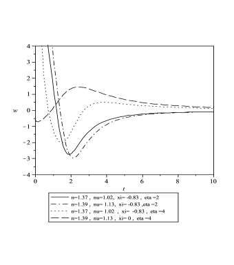
Figure 5: Crossing of $\omega=-1$ line in $F(R,\phi)=\frac{1}{2}(1-\xi\phi^{2})\ell_{0}R^{n}$   DGP-inspired model. As the figure shows, with a single minimally coupled scalar field there are regions of parameter space with no crossing of phantom divide line.

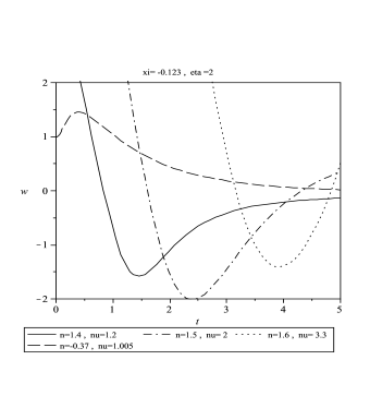
Figure 6: Crossing of $\omega=-1$ line. This figure shows that negative values of $n$ cannot account for phantom divide line crossing in this non-minimal setup.

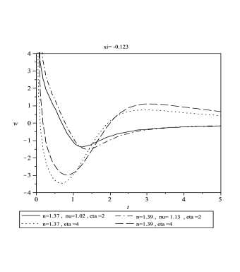
Figure 7: Crossing of $\omega=-1$ line in $F(R,\phi)=\frac{1}{2}(1-\xi\phi^{2})\ell_{0}R^{n}$ DGP-inspired model for different scalar field potentials and negative non-minimal coupling.

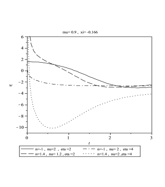
Figure 8: Crossing of $\omega=-1$ line in $F(R,\phi)=\frac{1}{2}(1-\xi\phi^{2})\Big{[}R-(1-n)\zeta^{2}\Big{(}\frac{R}{\zeta^{2}}\Big{)}^{n}\Big{]}$ DGP-inspired model for different scalar field potentials and negative non-minimal coupling.

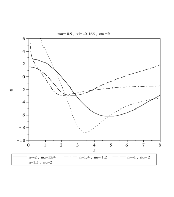
Figure 9: Crossing of $\omega=-1$ line in $F(R,\phi)=\frac{1}{2}(1-\xi\phi^{2})\Big{[}R-(1-n)\zeta^{2}\Big{(}\frac{R}{\zeta^{2}}\Big{)}^{n}\Big{]}$ DGP-inspired model for different $n$ and negative non-minimal coupling.

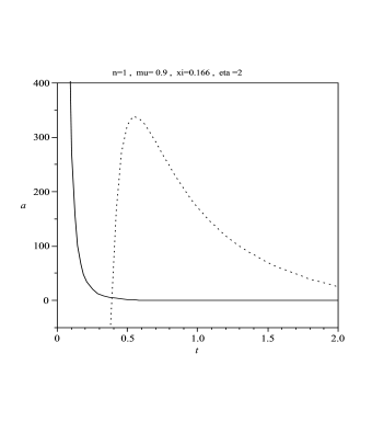
Figure 10: With $\eta=2$, $\xi=0.166$ and $n=1$, we find $\nu=1.2$ from equation (38). There is an intersection point between curves corresponding to two sides of this equation with $\nu=1.2$ accounting for positively accelerated expansion within $F(R,\phi)=\frac{1}{2}(1-\xi\phi^{2})\Big{[}R-(1-n)\zeta^{2}\Big{(}\frac{R}{\zeta^{2}}\Big{)}^{n}\Big{]}$ scenario.

5 Summary and Conclusions

Current positively accelerated expansion of the universe could be the result of a modification to the Einstein-Hilbert action. Also DGP braneworld scenario has the capability to interpret this late-time acceleration via leakage of gravity to extra dimension in its self-accelerating branch. On the other hand, there are several compelling reasons for inclusion of an explicit non-minimal coupling of scalar field and induced gravity on the brane sector of DGP action [14,16]. These arguments have led us to study cosmological implications of a DGP-inspired $F(R,\phi)$ gravity. Although this issue has been studied extensively for the minimal case, our setup provides a new approach to treat accelerated expansion within a general framework of modified scalar-tensor theories taking into account the role played by curvature correction and non-minimal coupling of scalar field and modified curvature simultaneously. We have studied late-time acceleration and possible crossing of phantom divide line in this setup. The condition for accelerated expansion and also equation governing on the dynamics of equation of state parameter are very complicated, so that we were forced to try a reliable and natural ansatz to find some intuition. We have shown that this setup accounts for accelerated expansion with a suitable choice of parameters space or fine-tuning. Also, this setup accounts for crossing of phantom divide line in some ranges of parameters appeared in the model. In the minimal case, our model coincides with existing models of $f(R)$ gravity. Especially the case with $n=-1$ in the absence of non-minimal coupling exactly coincides with well-known result [21]. On the other hand, for a single scalar field with minimal coupling to gravity there are region of parameter space with no phantom divide line crossing. We have seen in the numerical calculations that with $V(\phi)=\lambda\phi^{\eta}$, for both $\eta=2$ and $\eta=4$ and with arbitrary $\xi$, there is no crossing of phantom divide line for negative values of $n$ ( Figure $6$ ). However positively accelerated expansion of the universe can be explained in this situation with negative $n$. On the other hand, if $1.37\leq n<2$, for negative $\xi$ we have crossing of the phantom divide line ( see figure $7$ ). As an important result in the analysis of late-time behavior, from equation (27) we find that only for positive values of $n$ with $1.37\leq n<2$ and for positive or negative values of $\xi$, there are intersection points and therefore accelerated expansion for corresponding parameters choice. The case with $n=1$ which describes ordinary general relativity has been treated separately. By adopting more general theories such as $F(R,\phi)=\frac{1}{2}(1-\xi\phi^{2})\Big{[}R-(1-n)\zeta^{2}\Big{(}\frac{R}{\zeta^{2}}\Big{)}^{n}\Big{]}$, the previous restriction on $n$ is relaxed so that $n=1$ is a natural subset of the model. In summary, accelerated expansion can be explained by both positive and negative values of $n$ with suitable fine-tuning of other parameters. On the other hand crossing of phantom divide line in  $F(R,\phi)=\frac{1}{2}(1-\xi\phi^{2})\ell_{0}R^{n}$ model can be explained only with positive values of $n$ and fine-tuning of other parameters. The range of variation of $n$ to have crossing of phantom divide line in this setup is $1.37\leq n<2$. However in theories with $F(R,\phi)=\frac{1}{2}(1-\xi\phi^{2})\Big{[}R-(1-n)\zeta^{2}\Big{(}\frac{R}{\zeta^{2}}\Big{)}^{n}\Big{]}$ this crossing occurs for both negative and positive values of $n$. For theories of the type $F(R,\phi)=\frac{1}{2}(1-\xi\phi^{2})\Big{[}R-(1-n)\zeta^{2}\Big{(}\frac{R}{\zeta^{2}}\Big{)}^{n}\Big{]}$, $n$ is not restricted to this interval and these theories account for phantom divide line crossing even for negative values of $n$ as figure $9$ shows. The issues of ghost instabilities and violation of positive energy theorems have been discussed also. Due to wider parameter space as a result of non-minimal coupling of scalar field and modified gravity, we hope this model can evade these problems.

Acknowledgment We are indebted to an anonymous referee for his/her important contribution in this work.

References

- [1] A. G. Riess et. al. (Supernova Search Team Collaboration), Astron. J. 116 (1998) 1006, [astro-ph/9805201]; S. Perlmutter et. al., Astrophys. J. 517 (1999) 565, [astro-ph/9812133]; D. N. Spergel et. al., Astrophys. J. Suppl. 148 (2003) 175, [astro-ph/0302209]; C. L. Bennett et. al., Astrophys. J. Suppl. 148 (2003) 1, [astro-ph/0302207]; C. B. Netterfield et. al., Astrophys. J. 571 (2002) 604, [astro-ph/0104460]; N. W. Halverson et. al., Astrophys. J. 568 (2002) 38, [astro-ph/0104489]; D. N. Spergel et al, WMAP Three Year Results: Implication for Cosmology, [arXiv:astro-ph/0603499].
- [2] E. J. Copeland, M. Sami and S. Tsujikawa, Int. J. Mod. Phys. D 15 (2006) 1753-1936, [arXiv:hep-th/0603057].
- [3] T. P. Sotiriou and V. Faraoni, [ arXiv:0805.1726].
- [4] C. Deffayet, G. Dvali and G. Gabadadze, Phys. Rev. D 65 (2002) 044023, [ arXiv:astro-ph/0105068].
- [5] T. Padmanabhan, Phys. Rept. 380 (2003) 253; V. Shani and A. A. Astarobinsky, Int. J. Mod. Phys. D 9 (2000) 373; S. M. Carroll, Living Rev. Rel. 4 (2001) 1.
- [6] S. Nesseris and L. Perivolaropoulos, JCAP 0701 (2007) 018; [arXiv:astro-ph/0610092].
- [7] S. Capozziello, V. F. Cardone and A. Troisi, JCAP 0608 (2006) 001, [arXiv:astro-ph/0602349]; S. Capozziello, S. Nojiri and S.D. Odintsov, Phys. Lett. B 634 (2006) 93, [arXiv:hep-th/0512118]; S. Capozziello, V. F. Cardone, E. Piedipalumbo and C. Rubano, Class. Quant. Grav. 23 (2006) 1205, [arXiv:astro-ph/0507438]; S. Capozziello, V. F. Cardone, S. Carloni and A. Troisi, Int. J. Mod. Phys. D12 (2003) 1969, [arXiv:astro-ph/0307018].
- [8] M. Bouhmadi-Lopez and P. Vargas Moniz, [arXiv:0804.4484]; M. Bouhmadi-Lopez, [arXiv:astro-ph/0512124].
- [9] R. Gannouji, D. Polarski, A. Ranquet and A. A. Starobinsky, JCAP 0609 (2006) 016, [arXiv:astro-ph/0606287]; O. Hrycyna and M. Szydlowski, Phys. Lett. B651 (2007) 8, [arXiv:0704.1651]; O. Hrycyna and M. Szydlowski, Phys. Rev. D76 (2007) 123510, [arXiv:0707.4471]; M. Szydlowski, O. Hrycyna and A. Kurek, Phys. Rev. D 77 (2008) 027302, [arXiv:0710.0366]; S. Nojiri, S. D. Odintsov and P. V. Tretyakov, [ arXiv:0710.5232]
- [10] K. Atazadeh, M. Farhoudi and H. R. Sepangi, Phys. Lett. B 660 (2008) 275, [arXiv:0801.1398]; K. Atazadeh and H. R. Sepangi, JCAP 09 (2007) 020, [arXiv:0710.0214].
- [11] A. Vikman, Phys. Rev. D 71 (2005) 023515, [astro-ph/0407107]. See also other papers which accepted almost this viewpoint: Y. H. Wei and Y. Z. Zhang, Grav. Cosmol. 9 (2003) 307; V. Sahni and Y. Shtanov, JCAP 0311 (2003) 014; Y.H. Wei and Y. Tian, Class. Quantum Grav. 21 (2004) 5347; F. C. Carvalho and A. Saa, Phys. Rev. D 70 (2004) 087302; F. Piazza and S. Tsujikawa, JCAP 0407 (2004) 004; R-G. Cai, H. S. Zhang and A. Wang, Commun. Theor. Phys. 44(2005) 948; I. Y. Arefeva, A. S. Koshelev and S. Y. Vernov, Phys. Rev. D 72 (2005) 064017; A. Anisimov, E. Babichev and A. Vikman, JCAP 0506 (2005)006; B. Wang, Y.G. Gong and E. Abdalla, Phys. Lett. B 624 (2005) 141; S. Nojiri and S. D. Odintsov, hep-th/0506212; S. Nojiri, S. D. Odintsov and S. Tsujikawa, hep-th/0501025; E. Elizalde, S. Nojiri, S. D. Odintsov and P. Wang, Phys. Rev. D 71 (2005) 103504; H. Mohseni Sadjadi, Phys. Rev. D 73 (2006) 063525; W. Zhao and Y. Zhang, Phys. Rev.D 73 (2006)123509; P. S. Apostolopoulos and N. Tetradis, hep-th/0604014; I. Ya. Arefeva and A. S. Koshelev, hep-th/0605085; S. D. Sadatian and K. Nozari, Europhys. Lett. 82 (2008) 49001.
- [12] H. Zhang and Z.-H. Zhu, Phys. Rev. D 75 (2007) 023510, [arXiv:astro-ph/0611834]
- [13] K. Nozari, N. Behrouz and B. Fazlpour, [arXiv:0808.0318]
- [14] K. Nozari, JCAP 09 (2007) 003, [arXiv:hep-th/07081611].
- [15] A.G. Riess et al., Astrophys. J. 607 (2004) 665.
- [16] V. Faraoni, Phys. Rev. D 62 (2000) 023504, [arXiv:gr-qc/0002091]; V. Faraoni, Phys. Rev. D 53 (1996) 6813.
- [17] M. Ito, Europhys. Lett. 71 (5) (2005) 712
- [18] T. Chiba, Phys. Rev. D 60 (1999) 083508
- [19] K. Nozari and S. D. Sadatian, [arXiv:0710.0058], to appear in Mod. Phys. Lett. A.
- [20] S. Capozziello, Int. J. Mod. Phys. D11 (2002) 483, [arXiv:gr-qc/0201033]; S. Carloni, P. K. S. Dunsby, S. Capozziello and A. Troisi, Class. Quant. Grav. 22 (2005) 4839, [arXiv:gr-qc/0410046].
- [21] S. M. Carroll, V. Duvvuri, M. Trodden, M. Turner, Phys. Rev. D 70 (2004) 043528, [astro-ph/0306438].
- [22] K. Koyama, Class. Quantum Grav. 24, R231 (2007) [arXiv:hep-th/0709.2399].
- [23] C. de Rham and A. J. Tolley, JCAP 0607, 004 (2006) [arXiv:hep-th/0605122].
- [24] V. Sahni and Y. Shtanov, JCAP 0311 (2003) 014, [arXiv:astro-ph/0202346]
- [25] U. Alam and V. Sahni, [arXiv:astro-ph/0209443].
- [26] A. Lue and G. D. Starkman, Phys. Rev. D 70 (2004) 101501, [arXiv:astro-ph/0408246].
- [27] A. Lue, Phys. Rept. 423 (2006) 1, [arXiv:astro-ph/0510068].