Higgs Boson Production in Association with Multiple Hard Jets
Abstract:
We elucidate a new technique for estimating the production of multiple (at least two) hard jets in Higgs production via gluon-gluon fusion. The approach is based upon high energy factorisation, with the region of applicability extended by constraints on the analytic behaviour of the scattering amplitudes stemming from known all-order results. The method approximates both real and virtual corrections, and allows for the resummation in an -parton inclusive event sample of the terms dominant in the high energy limit. The resulting approximation is matched to the known tree level matrix elements for the production of a Higgs boson in association with 2 and 3 jets, and implemented in a Monte Carlo generator. Example results are presented and characteristic radiation patterns discussed.
NIKHEF-2008-010
1 Introduction
One of the main goals of the forthcoming Large Hadron Collider (LHC) will be to study the nature of the electro-weak symmetry breaking (EWSB). If a fundamental scalar is observed, one must determine whether or not it is the Higgs boson, responsible for the EWSB in the Standard Model. Thus, it is imperative to measure its couplings as accurately as possible, especially to the gauge vector bosons. This is possible by observing its decay to vector bosons, or by isolating the process of a Higgs boson production via vector-boson fusion (VBF). The latter contributes to the general signal of a Higgs boson in association with two jets, which also receives a significant contribution from Higgs boson production via gluon-gluon fusion (GGF), where the Higgs boson couples to gluons via a top quark loop. The large cross section associated with GGF makes it a valuable discovery channel in its own right [1]. However, a precise determination of the coupling of the Higgs boson to the weak gauge boson requires a suppression of the GGF contribution to the production of a Higgs boson in association with two jets. This can be achieved with the vector-boson fusion cuts of Ref. [2]. It is expected that the contribution from the GGF process can be further diminished by vetoing jet activity in the central rapidity region [3, 4], owing to the fact that GGF has a -channel colour octet exchange as opposed to the colour singlet of VBF.
The angular structure of the final state is very different in the VBF and GGF processes at lowest order. One expects a significant azimuthal correlation between the two jets in the GGF case, which is not so for VBF [2, 5]. The nature of the correlation contains information about the CP properties of the coupling of the Higgs boson to fermions or gauge bosons. The practical usefulness of this correlation is potentially threatened, however, by multiple hard jet emission which acts to decorrelate the jets. Thus it is clearly important to thoroughly understand the multijet final states in GGF.
There are several established methods for estimating the production of a Higgs with a number of accompanying partons. The first and best verified approach is to calculate the processes in fixed-order perturbation theory, up to as high an order in the strong coupling constant as is possible. For the VBF process, radiative corrections have been calculated both within QCD [6, 7, 8, 9, 10, 11] and the electro-weak sector [12, 13]. The radiative corrections to the VBF channel are small, and there is even partial numerical cancellation between the QCD and electro-weak contributions. Recently, the quantum mechanical interference between QCD and electro-weak Higgs boson production[14] was also investigated[15, 16].
Higgs boson + 2 jet production was computed at leading order in with full top-mass dependence in Ref. [17, 2], and in the large top mass limit in Ref. [18]. In the limit of infinite top mass, the coupling of the Higgs boson to gluons through a top quark loop can be described by a point interaction[19, 20, 7]. This approximation has been applied in most studies of Higgs boson production in association with jets, and will be applied also in the present one, although this is not essential to the approach. The large top mass limit is valid as long as the transverse energy of all the associated jets is smaller than the Higgs and the top masses[21]111For jet transverse energies larger than or , the full top-mass dependence must be taken into account. Beyond leading order, that dependence is known only in the limit of high partonic centre-of-mass energy[22]..
In the large top mass limit, the radiative corrections to Higgs boson + two parton final states were evaluated in Ref. [23, 24, 25, 26] and Higgs boson + 2 jet () production was calculated at full next-to-leading order (NLO) in Ref. [27]. Higgs boson + 3 jet () production is known only at leading order in [23]; it is unlikely that the process will be available at full NLO in the near future. Likewise, no full tree-level prediction for the production of a Higgs boson in association with four jets has yet been presented.
One method for estimating the effects of perturbative corrections beyond these lowest orders is to interface higher order tree level matrix elements with a parton shower algorithm, which estimates the part of the radiative corrections arising from soft and collinearly enhanced regions of the real emission phase space. This entails a marked dependence of the jet cross section on the parton-level generation cuts, and in particular an unphysical behaviour of the real emission elements as the of a jet tends to zero. Collinear and soft singularities are generated, which in a true NLO calculation would be cancelled by corresponding contributions in the virtual corrections. Such a technique was applied to Higgs boson production in [28], where the discussion was tailored towards isolating the VBF signal. In that study, real emission matrix elements for Higgs + parton production (where ) were interfaced with a parton shower, and it was found that in a significant fraction of two-jet final states one of the jets originated from the shower rather than the hard matrix element.
Thus, the question arises of whether it is possible to estimate multiparton final states using a method which captures the hard-parton behaviour of the multi-parton matrix elements to any order in . We present such an algorithm in this paper. Our starting point is the Fadin-Kuraev-Lipatov (FKL[29, 30, 31]) factorised form of multiparton amplitudes, an approximation to the full scattering amplitude which becomes exact in the limit of multi-Regge kinematics (MRK) with hard partons of infinite separation in rapidity, i.e. in the asymptotic limit when all interjet invariant masses tend to infinity. These amplitudes allow one to define exclusive multiparton final states, with the inclusion of virtual corrections whose singularities cancel those associated with soft real emissions. The conventional application of this framework, in the context of the Balitsky-Fadin-Kuraev-Lipatov (BFKL[32]) equation, applies the kinematical approximations everywhere in phase space, whilst integrating the evolution fully inclusively. By comparing the result order by order with the corresponding full fixed order results, we will demonstrate that this approach does not lead to a good approximation. However, we show that it is possible to modify the FKL framework to take into account the known structure of singularities of the full scattering amplitude to any order in the coupling. We thereby construct approximate scattering amplitudes, which have the same MRK limit as the FKL amplitudes, but maintain the correct position of singularities away from the high energy limit and thus better approximate the true amplitudes over all of phase space. One can view our approach as systematically building up approximate matrix elements, using FKL factorisation as a (hard) starting point, in contrast with applying a soft shower algorithm to a hard matrix element. Thus, our technique should be better suited at describing results sensitive to the jet multiplicity rather than the internal structure of each jet, which is best described by soft and collinear resummation.
We will validate our technique by comparing to known tree level matrix elements at low orders in . We then implement our prescription for calculating amplitudes in a Monte Carlo generator for Higgs boson production via GGF, where the tree level results for 2 and 3 parton final states are included via a matching procedure which avoids any double counting of radiation. This matching procedure could in principle be implemented at higher orders in . However, the evaluation of full tree level matrix elements becomes computationally punitive for more than 3 jets.
The structure of the paper is as follows. In section 2, we introduce the GGF process using LO results. In section 3, we introduce the factorisation properties of amplitudes in the high energy limit (HEL), before discussing the traditional BFKL implementation of this framework, applied to Higgs boson production via GGF in association with at least two jets. We then present our alternative implementation, based on the imposition of known analytic constraints, and validate the approach by comparing order by order in with fixed order results. In section 4, we discuss how the resummed amplitudes can be matched to the fixed order results at low orders in , and implemented in a Monte Carlo event generator. Some results from this generator are shown in section 5. Finally, in section 6, we summarise and discuss the possibilities for further systematic improvements.
2 Higgs Boson Production with Multiple Jets at Fixed Order
2.1 Production of Higgs + 2 Jets
The fully differential cross-section for the production of a Higgs boson with two accompanying partons may be written as follows:
| (1) |
where:
| (2) |
are the momentum fractions of the incoming partons; the transverse mass of the final state partons and Higgs boson; the corresponding rapidities. Here is the matrix element for production of a Higgs boson in association with partons and from partons and after averaging / summing over colour and helicity, is the squared partonic centre of mass energy, and the remaining numerical factors arise from the parameterisation of phase space.
Unless otherwise stated, we will concentrate on the contribution from QCD generated Higgs boson production within cuts optimised for the selection of events originating from the weak boson fusion process, as they were used in the NLO calculation of the QCD contribution to the -channel [27]. These are listed in Table 1.
| GeV | |||
| 4.5 |
As we will demonstrate, the good performance of the approximations we will make later does not rely crucially on these cuts - specifically we will also study events selected with a rapidity cut of just 2 units of rapidity.
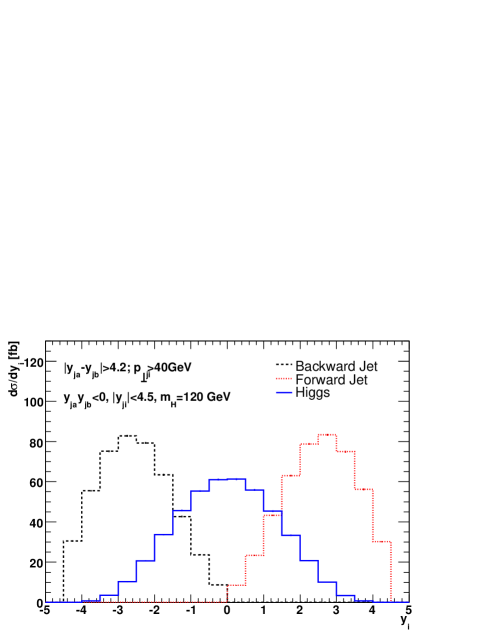
In Figure 1 we have plotted the rapidity distribution of the forward and backward jet, and the Higgs boson for the sum of all channels contributing to Higgs boson plus dijet production through gluon fusion at leading order. We use the following values for the Higgs boson mass, vacuum expectation value of the Higgs boson field and top quark mass respectively:
| (3) |
We also include a factor multiplying the effective Higgs boson vertices, accounting for finite top-mass effects [33]:
which increase the cross section by 5.9% for the parameter values in Eq. (3). Furthermore, we choose the NLO set of parton density functions from Ref.[34] (for all the studies presented here), and choose factorisation and renormalisation scales equal to . However, the resummation and approximation presented later is based explicitly on the kinematical part of the amplitude, and not on the running coupling terms. Thus, it does not relate to any specific scale choice, at least to the discussed accuracy. Tree level matrix elements have been obtained using MadGraph[35]. We report results for a 14 TeV -collider.
We find the tree-level cross-section from the QCD generated -channel to be fb, where the uncertainty is obtained by varying the common factorisation and renormalisation scale, as given above, by a factor of two. The variation is far less if the renormalisation and factorisation scales are varied simultaneously in opposite directions, where we find fb.
2.2 Observables for Distinguishing VBF and GGF
For a large rapidity-separation of the two jets, Higgs boson production via gluon fusion is dominated by a -channel exchange. The different structures of the and vertices (where is a or boson) give rise to different azimuthal correlations of the two leading jets. While VBF has a very mild dependence on the azimuthal angle between the two jets, for the GGF process the azimuthal correlation between the two jets exhibits a characteristic dip at [2]. However, it is expected that higher order corrections will somewhat fill the dip, thereby decreasing the discriminating power. The effect of such higher order corrections were estimated in Ref.[28] using a parton shower approach to resum the soft and collinear radiation. It is the purpose of this current study to calculate the effect caused by the emission of several hard gluons, which obviously can result in more decorrelation. In the following two subsections we will introduce some of the suggested variables for discriminating the QCD and VBF contributions to .
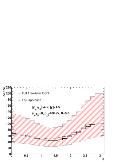
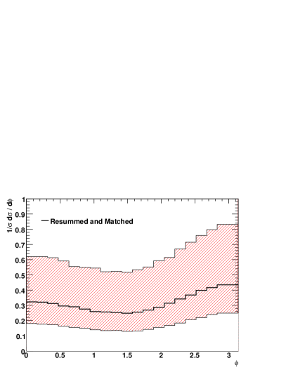
2.2.1 Azimuthal angle distribution
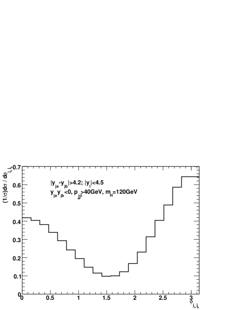
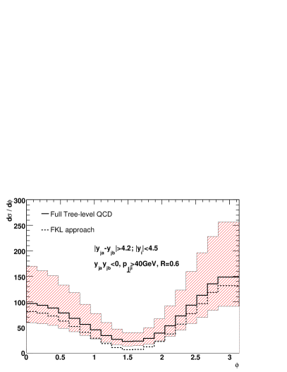
The LO result for the azimuthal angle distribution in production via GGF is shown in Fig. 2, for the Standard Model Higgs boson with -even couplings to two gluons, and shows the characteristic dip mentioned above. By contrast, the contribution from the VBF channel is much flatter (see e.g. Ref [5]).
2.2.2
As suggested in Ref.[5] the structure of the distribution can be distilled into a single number given by:
| (4) |
According to this definition, one has , with representing no azimuthal correlation between the tagging jets. A -even coupling for the vector boson fusion into a Higgs boson leads to a positive value for , whereas a -odd coupling results in a negative value. The Standard Model coupling for the weak gauge boson leads to in the VBF-sample. Using our standard cuts and scale choice in the GGF sample of a Higgs boson plus two partons, we obtain , in agreement with the CP-even nature of the effective coupling between the Higgs boson and two gluons, and the dominance of the -channel gluon fusion processes within the QCD contribution.
2.3 Production of Higgs + 3 Jets
By analogy with equation (1), the fully differential cross-section for the production of a Higgs boson with three accompanying partons may be written as follows:
| (5) |
where are the transverse momenta of the final state partons, and their rapidities.
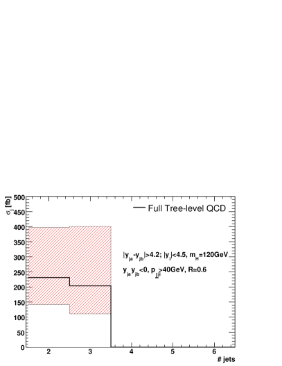
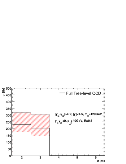
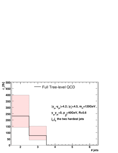
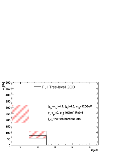
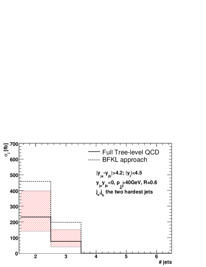
We start by considering the fully inclusive 3-hard-jet radiative correction to the two jet sample. By this we mean that an event with 3 hard jets will be accepted, if two of the jets fulfill all the requirements of Table 1. Contrary to the case for the 2-jet calculation with these cuts, the jet algorithm is relevant in defining the phase space for the 3-jet configuration. We choose the -algorithm as implemented in Ref.[36], with and using the energy recombination scheme. With the relevant cuts, and by evaluating the extra coupling compared to the two-jet case at scale , we find the leading order cross section for the production of Higgs Boson plus three jets to be fb. The uncertainty obtained by varying the factorisation and renormalisation scales in opposite directions is far smaller, resulting in an estimate for the cross section of fb. The requirement of an extra jet with the accompanying -suppression leads to a change in the tree-level cross section of less than 12%! In Figure 3 we have plotted the tree-level results for the and processes. The shaded bands indicate the size of the renormalisation and factorisation scale uncertainty obtained by varying the factorisation and renormalisation scales by a factor of two, either as a common scale (left) or in opposite directions (right). The full NLO K-factor for with this set of cuts is found to be 1.7-1.8222We thank John Campbell for this information.. The value of obtained with this 3-jet sample is , significantly lower than the leading order two-jet value.
The apparent lack of suppression of the three parton final state using the cuts of Table 1 has led to the alternative suggestion that when events containing three jets or more are considered, one should require that the two hardest jets in the event also satisfy the rapidity separation constraint [8, 23, 27, 10]. This significantly reduces the accepted three-jet phase space: A central jet will have a slightly harder transverse momentum spectrum than any forward jet, simply because of the smaller impact on the parton momentum fraction of a hard central jet, and the resulting lack of suppression from the PDFs. We will return to this point in Section 5.3. Therefore, if considering only the two hardest jets in the event, one is less likely to satisfy the rapidity separation constraint. For the above parameters we find fb (fb when varying the scales in opposite directions). The NLO K-factor obtained in the calculation of Ref.[27] with this set of cuts is 1.3-1.4, the difference with respect to the previous case obviously arising from the reduced three-jet phase space. The value of for this set of three-jet cuts is , i.e. much closer to the value found for the 2-jet sample.
The reason for the lack of a suppression in the 3-jet rate compared to the 2-jet rate of order is simply due to the large size of the -body phase space compared to the -body equivalent. At the LHC, and when a large rapidity span is already required, the balance between the impact of additional central jets on the parton momentum fractions followed by a PDF (and ) suppression and the increase in -body phase space can be such that the additional emission is not suppressed. We have here demonstrated this at the lowest orders in perturbation theory. Notice that the large size of the 3-jet rate is not due to a divergent matrix element (the divergent region is explicitly cut out by the jet algorithm and the requirement of all three jets having a significant transverse momentum), but is simply a well-behaved matrix element integrated over a large phase space. In order to stabilise the perturbative series by resumming the effects of a large -body phase space to all orders, we would need to construct an approximation (since we cannot calculate exactly to all orders) to the -leg, -loop amplitude, including the hard-parton region. This is the aim of the next section.
3 High Energy Factorised Matrix Elements and Inclusive Jet Samples
In this section we will outline how we can arrive at a useful approximation for the -leg, -loop amplitude relevant for the calculation of Higgs boson production in association with jets. We will start by general observations based on the analyticity of the S-matrix[37, 38, 39] for -particle scattering in a certain kinematical limit. We will extend the region of applicability for the results obtained in this limit to all of phase space, by further restricting the analytic behaviour of the amplitudes away from the specific limit. The amplitudes thus obtained will allow for a resummation of the leading behaviour as the Mandelstam variable , with fixed, perturbative transverse scattering momenta. We will demonstrate explicitly that the dominant contribution to the multi-jet cross section is captured within this framework, by comparing order-by-order with the results obtained in the previous section.
We will discuss the traditional implementation of the framework through the BFKL equation[32], and explain why this fails to reproduce the results obtained in the fixed order approach, even if it is built upon the same asymptotic limit as the framework presented here.
3.1 FKL Factorisation
It has long been known (see e.g. [40, 41] and references therein) that in any Lorentz-invariant quantum field theory, the scattering amplitude for scattering in the Regge limit of large centre of mass energy and fixed momentum transfer assumes the form
| (6) |
where and depend on the dynamics of the underlying theory. The generalisation to -scattering in the double-Regge limit of , fixed was expected to be
| (7) |
For the specific case of QCD, this factorisation was shown explicitly to hold [42] for general QCD multi-gluon amplitudes in a multi-Regge limit (i.e. all tending to infinity) to all orders in . It was later proved to hold also when one invariant mass is allowed not to tend to infinity[43]. The factorised amplitudes allows one to calculate the behaviour of the scattering as for fixed scattering momenta (of typical size ) to leading and next-to-leading logarithmic accuracy in . To leading logarithmic accuracy, one needs only to take into account the dominant contribution as all , which arises from processes with only gluon quantum numbers exchanged in the -channel(s). In the present study we will work only within this approximation.
We will denote the QCD amplitudes derived from the multi-Regge limit the FKL-amplitudes (Fadin-Kuraev-Lipatov), after the people who proved[29] the factorisation property and derived the form of and in QCD. It is found in this case that the function factorises further into functions of non-overlapping momenta. We will denote by FKL factorisation the factorisation of QCD amplitudes into a product of building blocks of the form (at LL, and similarly at NLL) in the limit of all , fixed.
It is worth noting that the VBF cuts of Table 1 approach at least the limit of large invariant mass between two particles, since a large rapidity span of the event is required. However, in the calculation of cross sections, there will be no cut on the invariant mass between all pairs of particles, and so the multi-Regge limit is not necessarily approached. Our starting point for obtaining an approximation to the matrix elements will be the FKL amplitudes obtained in the multi-Regge limit, and we will later discuss how to extend their region of applicability outside the ultimate MRK limit, so that inclusive cross-sections can be calculated reliably.
The FKL factorised -gluon amplitudes, derived for the MRK limit, and adapted to include also the production of a Higgs boson with a rapidity between the produced jets, are given by
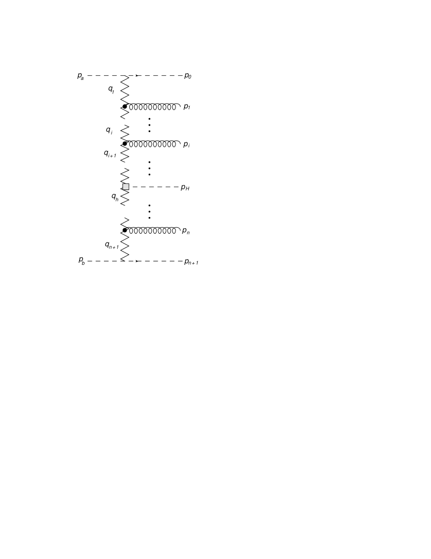
where is the strong coupling constant, and are the 4-momentum of gluon propagators (e.g. for ), is the Lipatov effective vertex, which at the leading logarithmic accuracy applied here results in gluon emission only (no quark-anti-quark pairs produced), and is the effective vertex for the production of a Higgs boson, as calculated in Ref.[21]. In Eq. (3.1), the rapidities of gluons are denoted with primes, if the rapidities are larger than that of the Higgs boson, such that we can set and for . The quantities occur from the Reggeisation of the gluon propagator, and encode virtual corrections (see e.g. Ref. [44]). We have suppressed the obvious Lorentz indices on the LHS of Eq. (3.1). This amplitude is pictorially represented in Fig. 5 - each zigzag -channel Reggeised gluon corresponds to a factor , and each real emission vertex corresponds to a factor . For the production of a Higgs boson outside (in rapidity) of the partons, we will use the equivalent factorised amplitudes with an impact factor for the production of a parton in association with a Higgs boson (see Ref.[21]), and gluon production vertices (no ) connecting to the far end of the ladder.
The MRK limit can be expressed in terms of the rapidities of the outgoing partons and their transverse momenta , so the MRK limit where the amplitudes of Eq. (3.1) become relevant is
| (9) |
Each emitted gluon is coupled to the -channel gluon exchange by a Lipatov effective vertex, given by (see e.g. Ref. [45]):
| (10) |
where etc., is the propagator denominator associated with the Reggeised gluon. The set of Feynman diagrams entering the calculation of the Lipatov vertex is gauge invariant up to subleading terms in the MRK limit. The MRK limit determines only the asymptotic form of the Lipatov vertex, and forms differing only by sub-asymptotic terms are often used, see e.g. Ref.[44, 46]. However, we will choose the form in Eq. (10), since it is manifestly Lorentz and gauge invariant in all of phase space, as discussed in Sec. 3.3. The exponential factors in Eq. (3.1) result from the Lipatov Ansatz for the Reggeisation of the -channel gluon propagator, which encodes the leading virtual corrections and contains the function,
| (11) |
with the number of colours. Note that the colour factors in equation (3.1) are derived for incoming gluons. The form of the amplitude is unchanged for incoming quarks apart from colour factors, such that the overall normalisation receives a factor if an incoming gluon is replaced by a quark [47]. This arises from the fact that in the MRK limit the coupling of the -channel gluons to external particles is insensitive to their spin.
In equation (3.1), the effective vertex for Higgs boson production is given by:
| (12) | ||||
where the coefficients are given in [21], and we have not denoted colour factors. Here and are the -channel momenta entering the vertex, and the transverse mass of the Higgs. This result is derived in Ref.[21], and is valid for all values of the top mass. However, Eq. (12) simplifies in the large top mass limit , when the top quark loop coupling the -channel gluons to the Higgs boson can be replaced by a contact interaction. In this limit one finds:
| (13) |
As one would expect, this is the same result one would obtain by starting directly from the effective Lagrangian in this limit, which was used to obtain the fixed-order results of the previous section. We will adopt the large top-mass limit from now on, in order to make direct comparison with the fixed order results. However, it is clear that the limit of large top-mass is not a necessary ingredient of our approach. We will also multiply the effective vertex for Higgs boson production with the same factor of Eq. (2.1) used in the fixed-order analyses.
As stated above, Eq. (3.1) applies to the case when the Higgs boson is produced with a rapidity inbetween partons 0 and . When this is not the case, a similar factorised form still applies, but with one of the jet impact factors (that of the jet closest in rapidity to the Higgs boson) replaced by the impact factor for combined Higgs boson plus one jet production[21].
3.1.1 Contribution from Processes with a suppressed High Energy Limit
The above amplitudes dominate the cross-section for Higgs boson production with multiple partons in the MRK limit, which gives the leading logarithmic contribution to the cross section as with fixed scattering momentum. It is clear that only some of the possible partonic configurations are present i.e. those of the form:
| (14) |
where , and the partons are ordered according to increasing rapidity in both the initial and final states (but the Higgs boson rapidity is unconstrained). Thus, there are two types of contribution to the scattering amplitude which are absent. Firstly, those containing final state partons other than the incoming species and multiple gluons. Secondly, diagrams with the external parton content of Eq. (14), but where the final state partons are not ordered in increasing rapidity. These possibilities are shown schematically in Figure 6.

In order to be able to base approximate scattering amplitudes on the FKL description, one must first check that the missing partonic subprocesses do not give a significant contribution to the cross-section in the fixed order results. In Section 2.1 we evaluated -production at leading order using the cuts of Table 1 and the standard choice of scales. The result for the total cross section was 230fb. We have explicitly checked the contribution to this arising from non-FKL like parton configurations, and the result is 0.7fb, i.e. less than 0.3%.
The non-FKL contributions are so heavily suppressed in the two-jet channel because of the requirement of a large rapidity separation between the two jets. However, there is no requirement of a large separation between all three jets for the production of a Higgs boson in association with three jets. Here, there is a leading logarithmic FKL contribution to e.g. but not (with ordering of rapidity as indicated), and there is no contribution at all to channels such as . We will denote the contributing channels as FKL configurations. In Section 2.3 we evaluated the tree-level cross section for -production within the “inclusive” cuts to be 203fb. The contribution from non-FKL configurations is 19fb, i.e. less than 10%, even with no requirement of a large invariant mass between all three jets. When requiring the two hardest jets to satisfy the jet cuts, we found the cross section for -production to be 76fb. Within these cuts, the contribution from processes with a suppressed MRK limit is 6.0fb, less than 8%. One could worry about the growing trend of missing contributions. This arises as a result of calculating the contribution from an increasing number of jets within a fixed rapidity interval (e.g. the detector coverage), which automatically decreases the maximum invariant mass between each jet. Within the description of factorised amplitudes, many subleading channels could be included by directly applying the Feynman rules for Reggeised particle exchanges as derived in Ref.[48] and references therein. However, in the present study we will consider only the same underlying processes which enter the leading logarithmic BFKL resummation scheme, as a first test of the importance of the improvements we can make to the analytic behaviour of each amplitude.
We have established that the partonic channels included in the approximation scheme indeed do dominate the cross section within the cuts of Table 1 (and in Section 5.1 we will see that the description is equally good for less stringent cuts). It is perhaps surprising that the approximation works so well also in the three-jet case, but the requirement of individual jets could act as a sufficient requirement of a minimum invariant mass between partons to ensure the dominance of the terms taken into account by the FKL approximation.
3.2 Connection with the BFKL equation
The FKL result and the factorisation of amplitudes is proven in the MRK limit. The question remains of how to apply this result to the calculation of radiative corrections outside this limit i.e. with no restriction on inter-parton invariant masses.
In this section we will describe how the FKL framework is traditionally implemented through the use of the BFKL equation. We will compare the description so obtained order by order with the results obtained from a full tree level calculation of the production of a Higgs boson in association with two or three jets. We will implement the relevant BFKL description of this process using the formalism developed in Ref.[49], respecting energy and momentum conservation.
In the MRK limit, the virtual momenta are dominated by their transverse components such that . Thus, it is conventional to neglect the longitudinal components of the ’s when evaluating the propagators. Starting from a lowest order -parton amplitude, obtained by setting all exponential factors to unity in Eq. (3.1), the emission of an additional gluon between gluon and leads to a change in all the momenta, but also to the emergence of an extra factor in the squared amplitude:
| (15) |
In the MRK limit, with all longitudinal degrees of freedom suppressed, this factor becomes
| (16) |
Taking into account the colour factors and couplings, the effect of one emission (apart from a change in momenta to account for overall energy and momentum conservation) then reduces to an extra factor in the squared matrix element (summed and averaged over colours and spins) of:
| (17) |
The BFKL approximation for the term of the colour and spin summed and averaged matrix element squared for with the Higgs boson produced with a rapidity between that of the jets is (see also Ref.[21]):
| (18) |
and the approximation for the term of the colour and spin summed and averaged matrix element square for is:
| (19) |
In Eqs. (18)-(19), where counts the number of partons with a rapidity smaller than that of the Higgs, and .
The soft divergence for in the amplitudes of Eqs. (18)- (19) and their obvious multi-gluon generalisations is regulated by the soft-gluon divergence in the Reggeised propagators, as discussed in Sec. 3.3.4.
While the original factorisation of the amplitudes, and the form of the invariants used in deriving the results in Eqs. (18)-(19) are valid only in the MRK phase space region of
| (20) |
in the BFKL equation they are applied to the fully inclusive phase space, where the constraint on large rapidity separations between all partons is dropped. The simple form of Eqs. (18)-(19) (generalised to all orders), allows for the calculation of the approximate sum over and and the infinite phase-space integral of the emitted gluons in the squared amplitude of Eq. (3.1). The partonic cross section for e.g. as a function of the momenta of the Higgs boson and the extremal partons only then takes the following form:
| (21) | ||||
where is the solution of the BFKL equation, which has the form:
| (22) |
Here is the BFKL kernel, and the two-dimensional transverse part of 4-momentum (i.e. ). The implicit integrations over all of (rapidity ordered) momenta for the emitted gluons performed when solving the BFKL equation to find can create a problem though. In Eq. (LABEL:eq:BFKLapproximation), a factor of has been cancelled between the approximate squared matrix element and the flux factor in the partonic cross section. This might leave the impression that the resulting (partly integrated) partonic cross sections of Eq. (LABEL:eq:BFKLapproximation) do not depend on the momenta of the incoming particles. For a given final state configuration, the incoming momenta are of course given by momentum conservation. However, the final states which are integrated and summed over to arrive at Eq. (LABEL:eq:BFKLapproximation) arise from different initial state momenta, even if these cannot be reconstructed after the solution to the BFKL equation has been substituted. This is the problem of energy and momentum conservation in the BFKL formalism.
In order to obey factorisation when calculating hadronic cross sections, the parton distribution functions (PDF) must be evaluated at the light-cone momentum fractions of the incoming partons, which are relevant for the given final state momentum configuration. This requires the PDFs to be convoluted with the solution of the coupled BFKL equations in Eq. (LABEL:eq:BFKLapproximation) (thus altering the BFKL evolution), which can be achieved by solving the BFKL equation iteratively, through the method outlined in Ref.[50, 51, 52]. Specifically, we choose to follow the implementation advocated in Ref.[49]. These methods allow for a straightforward expansion of the solution in powers of . It is thereby easy to extract the contribution proportional to for 2-parton final states, and for 3-parton final states (these obviously agree with Eq. (18) and Eq. (19) respectively), and compare the results obtained for the 2 and 3-jet final states with those obtained using the full matrix element.
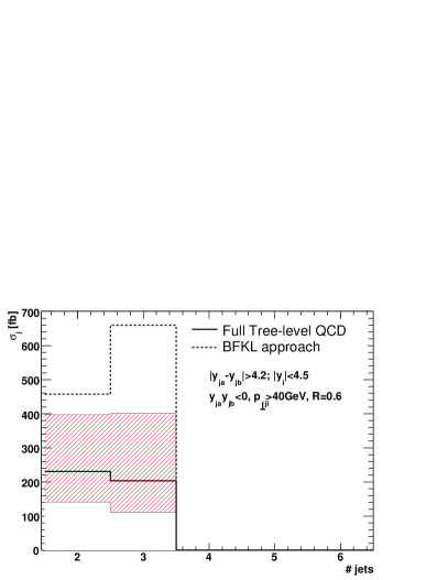
On Fig. 7 we have compared the results for the cross section for the production of a Higgs boson in association with two and three jets obtained within the BFKL approach with the results obtained for the full matrix elements in the FKL configurations (to be compared with Fig. 3). We find that the results based on the BFKL approximations for the (fb) and inclusive (fb) cross sections differ from their full leading order counterparts by and respectively. The kinematic approximations are clearly inadequate in describing amplitudes in general at the LHC. The matching corrections to a resummation based on these results would be uncomfortably large, and encourage very little trust in the predictions based on this approximation.
We note again that there is no restriction on the rapidity separation between the Higgs boson and any jet, nor between the rapidity of the middle (in rapidity) jet and any other object. So the BFKL amplitudes are here, just as in the BFKL equation, applied far outside of the MRK region.
The results of Figure 7 were found imposing 4-momentum conservation on the BFKL equation. However, this is traditionally neglected in the BFKL formalism since it is formally subleading in , and also because the BFKL equation explicitly requires the longitudinal momentum dependence to be dropped, which leads to violation of momentum conservation in all but the transverse components. However, such results are clearly not sensible, due to the unbounded phase space integration of the emitted gluons. It is easy to see that capturing just the dominating behaviour of the partonic cross section as , fixed will not describe correctly the large-invariant mass limit at a fixed energy collider: Consider the limit (i.e. the hadronic centre of mass energy), obtained when the final state partons of extremal rapidity become widely separated. This limit occurs before the strict Regge limit of is reached, and there is then no phase space left for the emission of additional gluons, and the kinematics return to that of the lowest order. This is not respected by any description based upon an analytic solution of the BFKL equation.
3.3 Modified High Energy Factorised Amplitudes
In the previous section, we saw that the BFKL implementation of the FKL factorisation formula does not accurately approximate fixed order matrix elements when applied over the phase space relevant to the LHC, even when energy and momentum conservation are implemented. In this section, we show that it is possible to modify the FKL description outside of the MRK limit, in such a way that its applicability can be extended. These modifications go beyond any logarithmic order in in the traditional BFKL expansion. The resulting amplitudes can be used as an approximation to scattering amplitudes with many final state partons, i.e. at orders in where fixed order perturbation theory is infeasible. This is analogous to the use of the soft- and collinear factorisation, which forms the basis of any parton shower Monte Carlo and most resummation formulae, outside of the strict soft and collinear region. Only outside the strict soft and collinear regions is there any observable effect of the radiation, and one then hopes that the results obtained in this limit are also relevant for a larger region of phase space. This is also the case in the present framework. However, because it does not rely on soft and collinear approximations, it should be better at describing the hard jet topology in an event, as opposed to the jet substructure. This section elaborates on the presentation in Ref.[46], although with some modifications to the formalism that we discuss in what follows.
We take as our definition of our approximate scattering amplitudes for + multiparton production the FKL factorisation formula (Eq. (3.1)), which is then applied subject to the following guidelines:
-
1.
Use of full virtual 4-momenta: Rather than substituting as in the BFKL equation and the original work of Fadin and collaborators, we keep the dependence on the full 4-momenta of all particles. This ensures that outside of the MRK limit, the singularity structure of the approximate amplitudes coincides with known singularities of the full fixed order scattering amplitude.
-
2.
Use of the Lipatov vertex as defined in Eq. (10). The results of the MRK limit constrains only the asymptotic form of the Lipatov vertex. Our choice for the sub-asymptotic behaviour is enforced by an added requirement of Lorentz invariance and fulfilment of the Ward identity throughout all of phase space. The latter condition is expressed by , where the minus sign arises from the gluon polarisation tensor.
These guidelines distinguish our approach from previous applications of the FKL factorisation formula, and thus we refer to our amplitudes from now on as modified FKL amplitudes. The above requirements do not impact on the logarithmic accuracy (in ) of the amplitudes, but enforce constraints on the sub-asymptotic behaviour stemming from known features of all-order perturbation theory.
3.3.1 Results for the Modified FKL Amplitudes
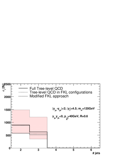
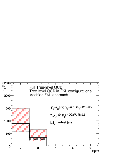
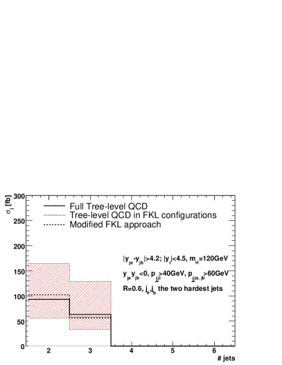
In Fig. 8 we have plotted the results obtained using the expansions to for and for of the matrix elements in Eq. (3.1), supplemented with the guidelines outlined above. We compare these with results obtained for the FKL configurations of full tree level QCD (dotted line), as discussed in subsection 3.1.1 and Figure 6, and with the results of all tree-level QCD configurations (full line). The same choice of renormalisation and factorisation scale () has been applied in both the modified FKL approximation and the full QCD results. To give a sense of the level of agreement between the FKL approximation and the full results, we indicate with the hashed band the scale uncertainty from varying the common renormalisation and factorisation scale by a factor of two in the full QCD result.
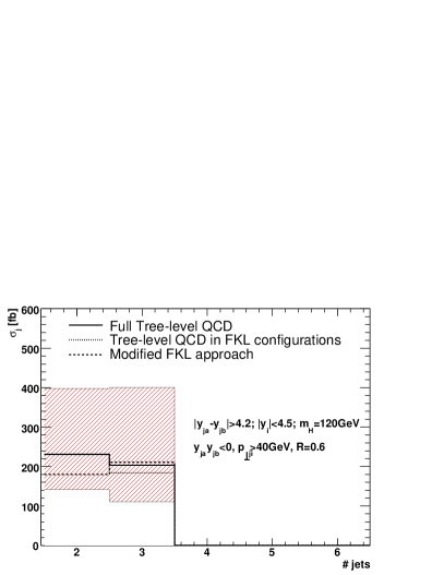
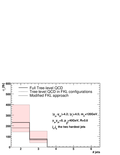
It is clear that the modified FKL amplitudes result in a much better approximation than those obtained using the BFKL description. The matching corrections in the BFKL approach of the previous section would be of the order of 100%, whereas the use of the modified FKL amplitudes results in matching corrections of less than 25% compared to both the result for FKL configurations only, and the sum over all subprocesses and rapidity configurations (i.e. the full result at LO). One sees that the LO and cross-sections (in FKL configurations) are produced to within 22% and 15% respectively in the case of the inclusive cuts, and within 22% and 6% respectively in the case of the hard cuts. We stress that the good agreement obtained is not specific to the particular choices made for either the cuts, or the renormalisation and factorisation scales. In Sec. 5.1 we will discuss results obtained with the requirement of a rapidity span reduced to 2 units of rapidity. The very good level of approximation obtained using the modified FKL prescription is important for several reasons: It gives a viable platform for building a resummation scheme, and it demonstrates that at least for the hard parton configurations considered here, there is no other source of large systematic effects not taken into account by the current prescription.
In the case of the Higgs boson produced in-between the jets (in rapidity), the three jet rates are in fact produced to a slightly better accuracy than the two-jet rates. This might seem strange, since the factorised three-jet formula builds on the factorised two-jet formula, and so one could expect the approximations to worsen order by order. However, in the -sample, the jets can have very different transverse scales, leading to a large variation of the ’s. In the three-jet sample, however, large transverse momenta are increasingly suppressed by constraints from the PDFs; the requirement of an extra hard jet limits the available transverse phase space. Therefore, the results for three-jet configurations approximate the full QCD better than the results obtained with the two-jet sample. A much better agreement for the two jet case arises when the Higgs boson lies outside the two jets in rapidity. The resulting FKL amplitude contains an impact factor for jet + Higgs boson production separated from another jet by the exchange of a single -channel Reggeised gluon with the transverse momenta on either side of the -channel propagator balancing, and the two-jet approximation is then found to be better than 1%! It is no surprise that the approximation works better in such cases; the factorisation assumes an infinite invariant mass between the system of one jet and a jet with the Higgs boson, rather than a infinite invariant mass between all particles. We note in passing that the mass of the Higgs boson introduces an extra scale to the problem, which is actually expected to worsen the quality of the approximations over the situation in a pure jet study.
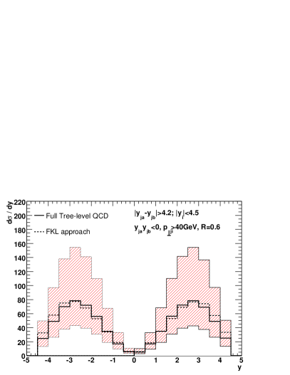
One must also check that kinematic distributions are well approximated by the formalism, and we show here some sample results for the LO and channels using the inclusive cuts of table 1. In figure 9 we show the rapidity distributions of the extremal partons, for the LO and . One sees that the modified FKL formalism agrees well with the full tree level results.

Similarly, the rapidity distribution of the central parton in is shown in figure 10, and that of the Higgs boson (for both and ) in figure 11.
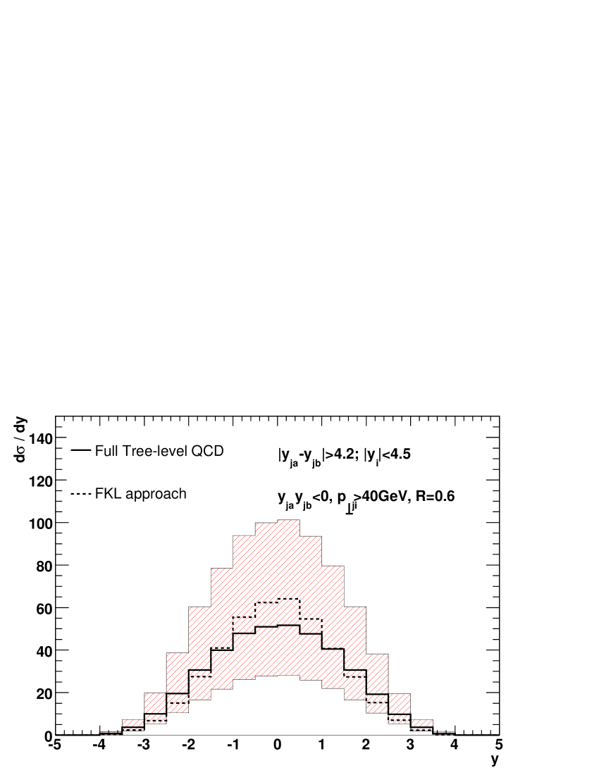
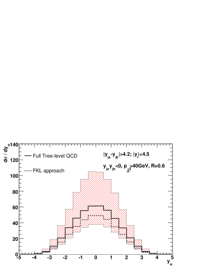

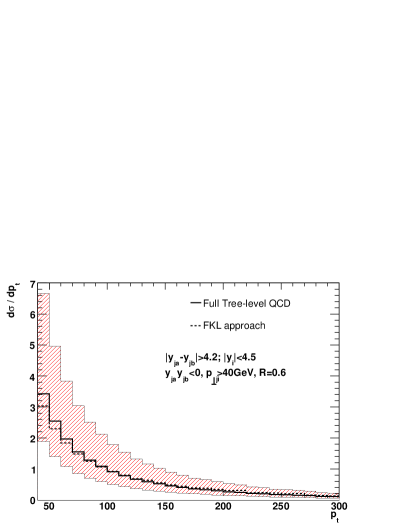
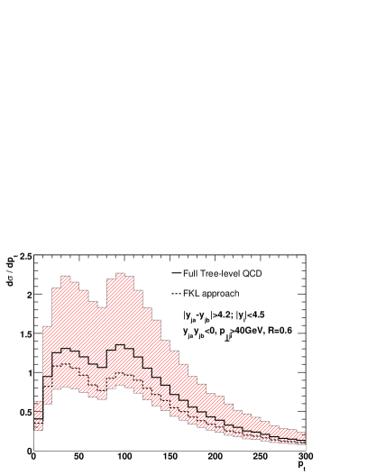
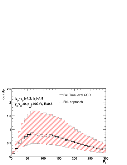
In figures 12, 13 and 14 we show the transverse momentum distributions for the extremal partons, central parton (in ) and Higgs boson respectively. The shape of the Higgs boson spectrum is discussed further in section 5.6. For now we note that there are large qualitative differences between the result for and . This is shown in figure 15.
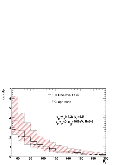
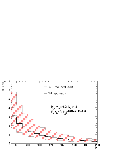
For each of the observables above, we find that shapes of distributions are generally well-estimated by the modified FKL formalism. Note that although the results in figures 9-15 have been presented for one choice of cuts (the inclusive cuts of table 1), we checked that a similar level of agreement was obtained for the other cut choices used in this paper.
Having validated our framework for estimating Higgs boson + multiparton scattering amplitudes, we now consider the physics motivations underlying the modifications to the FKL amplitudes presented in section 3.3.
3.3.2 Restoration of Analytic Properties and the Relation to Next-to-Leading Logarithmic Corrections
The argument for using the longitudinal (as well as transverse) components in evaluating the Reggeised gluon propagators (contrary to what is advocated in e.g. Ref.[43]) can be rationalised as follows. Firstly, as already hinted above, this restores the correct position of the divergences for the amplitude outside of the true MRK limit. This is obviously important when the amplitude is evaluated without any explicit requirement of infinite invariant mass between each and every parton. Using full propagators also removes the problem of diffusion [53] encountered in the BFKL formalism when , since this is not a special point for the FKL amplitudes. In fact, within the relevant physical region of phase space encountered at the LHC, the transverse momentum of the imagined -channel gluons vary to a much larger extent than the square of the full -channel 4-momentum . This immediately seems to endorse a setup tailored to the constraint of Eq. (9) rather than one using the constraints in Eq. (20).
Secondly, the next-to-leading logarithmic corrections to the Lipatov vertex begin to address the same issue, by reinstating the dependence on the longitudinal momenta - albeit only that part relating to the emission of two particles from the same Lipatov vertex at NLL. However, as long as the BFKL equation is kept (at either LL, NLL accuracy or beyond), a replacement of between each Lipatov vertex is performed, which ignores the longitudinal components of propagators connecting -vertices (this ensures that the BFKL equation depends only on the transverse momenta), and there is no information on longitudinal momentum flow between each Lipatov vertex. Therefore, the restoration of the full propagator is beyond any fixed logarithmic accuracy. For example, the full propagator for the matrix element for Higgs partons would never be restored in a description based on the BFKL equation. By completely avoiding the framework of the BFKL equation, we can implement these important corrections to any logarithmic accuracy (and beyond).
3.3.3 Connection to the Kinematic Constraint
The results of FKL constrain only the form of the square of the Lipatov vertex in the strict MRK limit, as given in Eq. (16). The use of any form differing only by sub-asymptotic terms (i.e. leading to the same asymptotic limit) is obviously allowed, if one is trying to maintain only a certain logarithmic (in ) accuracy. However, we would like to ensure a physical behaviour of the amplitudes in all of phase space (not just in the MRK limit), in order to construct an approximation which can be trusted to deliver reliable results for processes relevant for collider phenomenology, specifically with no requirement of infinite invariant mass between all partons. We choose to require gauge invariance (or fulfilment of Ward’s identity) and positive definiteness of the squared emission vertex, which severely constrains the sub-asymptotic terms. The former corresponds to the requirement , where is the emitted gluon momentum. It is easily verified from Eq. (10) that this is the case over all of phase space (i.e. not just in the MRK limit). Positive definiteness arises from the fact that as defined in Eq. (10) is a sum of light-like and space-like 4-vectors, and thus is itself space-like. The fact that is a 4-vector also implies that the squared emission vertex is Lorentz invariant. Other choices of vertex do not satisfy this property in general (although all are longitudinally boost invariant); the terms breaking Lorentz invariance and the gauge dependent terms are suppressed in the MRK limit. The extra constraints go beyond any fixed logarithmic accuracy, but are needed in order to enforce a correct physical behaviour of the scattering amplitudes, when applied to the calculation of scattering processes of relevance to collider phenomenology.
Other procedures for modifying the sub-asymptotic behaviour in the FKL formalism have been studied before. In Ref. [46], a different choice of the Lipatov vertex was used (that of Ref. [44]). This was not positive definite over all of phase space, and thus the constraint was additionally imposed. This removed a part of the sub-MRK phase space, and thus was related at least partially to the so-called kinematic constraint [54, 55] implemented in the CCFM equation [56, 57, 58]. Both approaches limit the region of phase space in which the factorised amplitudes are applied by requiring a varying degree of dominance of the transverse momenta over the longitudinal momenta of the -channel propagator momenta, and specifically apply to the sub-MRK behaviour of the result.
The kinematic constraint is most often discussed in connection with the small- evolution of parton distribution functions, and restricts the region where the BFKL evolution is applied on the basis of the -channel momenta and the transverse momenta of the gluons . Introducing the light-cone coordinates:
| (23) |
we consider an incoming parton with light-cone momentum . Then the kinematic constraint for the ’th -channel gluon can be given in terms of the light-cone momentum fractions:
| (24) |
In our study, we have incoming partons with both negative and positive light-cone momenta, so we will also need the negative light-cone momentum fraction
| (25) |
We note that the MRK limit corresponds to for all . We can now study three incarnations of the kinematic constraint, which require the momenta of the emitted partons and the -channel momenta to fulfill the following conditions ( can be either , or both, depending on the direction of the evolution)
-
1.
The form of Ref. [58]:
(26) - 2.
-
3.
The condition that the transverse components of the Reggeised momentum is larger than the longitudinal parts:
(28)
Radiation not fulfilling these inequalities is vetoed. All three constraints are trivially satisfied in the MRK limit.
Starting from the FKL-based approximation to the cross section, we collect in Table 2 the result of imposing the kinematic constraints mentioned above in the Higgs boson plus three-jet rate.
| Constraint | |
|---|---|
| None | 211 fb |
| 57 fb | |
| 33 fb | |
| 140 fb | |
| 97 fb | |
| 178 fb |
Without any constraint, the integrated cross section is 211fb (to be compared with the contribution from full LO QCD of 203fb). Imposing an additional kinematic constraint (absent in our current implementation of the FKL formula) can be seen to remove significant fractions of the (non-MRK) phase space, which is relevant to LHC physics, reducing the cross section by up to a factor of 6!
As expected, the weaker forms of the constraint cut out less of the phase space, but would still seem to be removing too many events to then be able to describe the cross-section well.
3.3.4 Regularisation of the Amplitudes
As shown in the previous sections, the modified FKL results for the and cross-sections agree well with the full fixed order matrix elements at low orders in . However, the aim of the framework is not just to reproduce known results, but to allow for an approximation of higher order amplitudes which are not calculable using present day full fixed order perturbative techniques. In order to be able to implement the resulting amplitudes in a numerical context, the cancellation between virtual divergences (from Eq. (11)) and those arising from real emission (when any ) must be made explicit.
We will consider the cancellation of divergences order by order in . For simplicity and without loss of generality, let us consider the divergence related to the middle gluon in going soft; again, without loss of generality we will take the rapidity of the middle gluon to be larger than that of the Higgs boson. In this case, in Eq. (3.1), and in the limit with all other outgoing momenta fixed we get:
| (29) |
The structure of divergences and their cancellation will turn out to be very similar to the one arising in the BFKL equation, and can be regularised using a phase space slicing method, which has been successful at regularising the iterative approach to solving the BFKL equation at LL [59, 51, 50] and NLL [60, 61]. By integrating over the soft part of phase space in dimensions, we find
| (30) | ||||
The divergence as is cancelled by the virtual corrections from the matrix element on the right hand side of Eq. (29), arising from the Reggeised -channel propagator between parton 0 and the Higgs boson. Indeed, one finds for (see e.g. [45])
| (31) |
The square of the matrix element on the left hand side of Eq. (29) contains the exponential . By expanding the exponential to first order in and in , the resulting pole in does indeed cancel that of Eq. (30), and one is left with a contribution
| (32) |
which is the regularised form of the exponent describing the virtual (and soft) emission in the FKL factorised amplitude of Eq. (3.1). It is clear that the nested rapidity integrals of additional soft, factorising radiation in multi-parton amplitudes will build up the exponential needed to cancel the poles from the virtual corrections to all orders in . The divergence arising from a given real emission is therefore cancelled by that arising from the virtual corrections in the Reggeised -channel propagator of the matrix element without the real emission.
3.3.5 Performing the Explicit Resummation
The regularisation discussed in the previous section allows one to construct fully inclusive event samples, where each event contains a Higgs boson and partons in the final state. The framework which emerges is therefore similar in application to the one suggested in Ref.[49] for solving the BFKL equation. Corrections beyond those entering the NLL BFKL kernel can be taken into account by applying directly the effective Feynman rules for Reggeised particles as discussed in Ref.[48]. This would automatically solve the problems associated with energy and momentum conservation in the NLL corrections to the BFKL kernel, as discussed in Ref.[62].
The regularised FKL amplitudes for incoming gluon states (quark states change only the colour factor) and the production of a Higgs boson between the extremal partons take the form (using the same notation as in Eq. (3.1))
with
| (34) |
In order to ensure the correct cancellation between real and virtual corrections, the matrix elements in Eq. (3.3.5) should always be used in fully inclusive samples. That is, in our studies we study the ensemble of partonic processes
| (35) |
where the parton densities and flux factor are omitted on the right-hand side for brevity. In this form, the cross section takes a form which is extremely similar to the equations for the iterative solution to the BFKL equation derived in Ref.[63, 49]. Only the integrand has changed in the description. This means that the phase space sampler for integrals of this sort developed in Ref.[49] can be applied in the calculation of the fully inclusive sample of Eq. (35). We choose to evaluate the fixed coupling in Eq. (35) at scale . In principle the effects of the running of the coupling could have been modelled according to Ref.[50]. However, we choose not to, anticipating instead to incorporate the full NLL corrections at a later stage.
The only unregulated divergence in this ensemble arises in the first and last bracket in Eq. (3.3.5) when . This divergence we have to regularise by restricting the transverse momentum at the impact factors. This ensures that our chosen framework remains appropriate. The divergence could also have been regularised by replacing the use of impact factors with unintegrated pdfs, thus avoiding a strict cut-off. However, a comparison with fixed order results would then be less straightforward.

On Fig. 16 we plot the resummed inclusive -jet cross section for three choices of the transverse momentum cut-off for jets, as a function of the minimum transverse momentum allowed for the parton arising from the impact factors. All three results have a similar shape. The cross section decreases with a universal slope, as the minimum transverse momentum for partons from the impact factors is increased above the minimum jet transverse momentum . There is a ‘heel’ in the spectrum for just below ; this is caused by a parton from the impact factors being just short of making it as a single jet, but combined with an additional parton emitted from the -channel evolution there is sufficient transverse momentum to qualify as a jet. As is lowered further, a plateau in the dependence is reached, followed by the universal divergence as . The separation between these regions is increasingly clear as the required hardness of the jets is increased. As discussed above, we want to remove as much dependence on the singularity at , since this behaviour would be regularised by effects not included in the current description. We do want to include the possibility of the partons from the impact factors (i.e. the partons extremal in rapidity) forming a jet with a parton from the evolution, giving rise to the heel in the distribution. We therefore impose a cut in the transverse momentum of the parton from the impact factor somewhere in the plateau region. In our studies we require the observed jets to have a transverse momentum of at least 40 GeV, and decide to allow for extremal partons down to 30 GeV. In this way, the partons emitted from the impact factors do not necessarily enter any jet - in other words, the “evolution” in rapidity is at least as long as the largest difference in rapidity between the observed jets.
4 Matching to Tree Level Matrix Elements
Given that the full tree level matrix elements for two and three parton states are computationally quick to calculate, they can be implemented alongside the modified FKL amplitudes and used to improve the description of Higgs boson production at low orders in . It is then necessary to define a suitable prescription for matching the perturbative expansion of the two and three jet rates obtained from the ensemble in Eq. (35) to the results obtained in fixed order perturbation theory point by point in phase space. In this way one corrects for both the contribution from non-FKL configurations, and for the difference between the approximation and the full result for the 2 and 3 jet rates in FKL configurations. If the virtual corrections to the 2-jet rate were known in a compact form, one could also match the ensemble to full -accuracy.
In practice this works as follows. Our Monte Carlo implementation will start by generating a random point in the full –particle phase space. It will then sum over each possible partonic channel, checking whether it corresponds to a FKL configuration. If so, it evaluates the appropriate scattering amplitude of Eq. (3.3.5) (with the colour factor in the impact factors replaced with for incoming and outgoing quarks). If the phase space configuration corresponds to a -parton final state, hard jet configuration for , it will then evaluate also the appropriate full tree-level matrix element, and apply a suitable matching correction to avoid any double counting of radiation.
We consider two distinct methods for matching, inspired by the so-called and -matching in Ref.[64]. We will describe the matching procedure for matrix elements with a two parton final state. The generalisation to the three parton final state is straightforward.
Let be the LO matrix element coming from the modified FKL approach i.e. this arises from Eq. (3.1) with the value of in the virtual corrections set to zero. Furthermore, let be the regularised (i.e. with virtual corrections included), modified FKL amplitude for (where the 2 partons form 2 jets), and the full tree-level result for . One may consider matching these quantities as follows:
| (36) |
i.e. instead of using the usual FKL amplitude for such a configuration, one modifies it to include the full tree level matrix element, and subtracts the LO part of the FKL amplitude. We call this -matching by analogy with Ref.[64].
Since the resummed virtual and unresolved corrections suppress a given -parton final state such that , it seems reasonable to also suppress the relevant matching corrections. This can be achieved by instead reweighting those events with a parton final state, n hard jet configuration according to the prescription:
| (37) |
This is formally equivalent to Eq. (36) up to the required order of the perturbation expansion. We call this -matching, since the correction is additive in the logarithm of the scattering amplitude. Effectively, this means that the exponentiated virtual corrections are also applied to the matching corrections.
In both - and -matching, the matching correction vanishes in the MRK limit, as it must do. Clearly, one can only apply -matching if the resummed matrix element is non-zero. For all other processes, one must use -matching. That is, -matching is used for those matrix element in which either (i) the partonic configuration is not FKL-like; (ii) the partonic species are FKL-like, but they do not satisfy the required rapidity ordering.
In principle the matching prescription described above can be extended to any number of hard jets (and indeed any order in the fixed order perturbation expansion). However, the computational evaluation of tree level matrix elements for the process considered here becomes very CPU intensive for more than 3 jets. So far, no estimates have been reported on the leading-order –jet cross section.
5 Results
In this section we present a few physics analyses arising from a Monte Carlo
event generator based on the resummation discussed in the previous sections,
supplemented with matching point by point in phase space to the full tree
level matrix elements for Higgs boson production with two and three jets. The
Multi-Jet EVent generator can be obtained at
http://andersen.web.cern.ch/andersen/MJEV.
5.1 Relations Between Rapidity Span and the Number of Hard Jets
The resummation leads to an increase in average jet activity with increasing rapidity length of the event. This effect is inherent to all -channel colour octet exchanges admitting this resummation, and independent of the specific process. In order to study this evolution over a longer rapidity range, we relax the cut on the rapidity separation between two jets. It is therefore relevant to start by asking how well the modified FKL amplitudes approximate the full fixed order results, if the cut is relaxed to a minimum separation of, say, two units of rapidity. In Figure 17 we plot the equivalent of Figure 8 with the cut in rapidity difference relaxed from 4.2 to 2 units of rapidity.
We see that even with such a small overall rapidity span required, the factorised formalism still describes the two and three-jet result of the full tree-level calculation in LL FKL configurations to better than 35% and 8% respectively for the standard cuts, and 35% and 16% for the hard cuts. This is quite remarkable, since the maximum rapidity distance between all jets at is just one unit of rapidity, and furthermore the Higgs boson is also often produced within the same rapidity interval, so the maximal invariant mass between each set of particles is not necessarily particularly large.
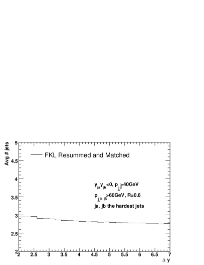
The -channel colour octet exchange has a characteristic radiation pattern, in terms of a correlation between the length in rapidity of the resummation (i.e. in Eq. (3.1)) and the average number of hard jets. This quantity is studied in Figure 18 (left) for the inclusive cuts, with defined as the rapidity span between the most forward and backward hard jet. We see that the average number of hard jets rises almost linearly from 2.6 to 4.1, as the rapidity length increases from 2 to 7.
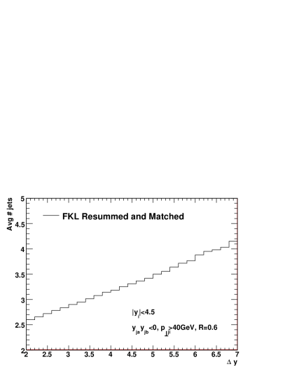

On Figure 18 (right) we study the average number of hard jets as a function of the rapidity difference between the two hardest jets, with the event selection based on the same two hard jets. Obviously, in this case the average jet count is smaller than with with inclusive cuts, but we also see that despite the same underlying physics used in the description, the correlation between average hard jet count and rapidity is partly changed by the choice of cuts, and partly masked by the definition of the rapidity variable. One now sees a decrease in the average number of hard jets, as the rapidity difference between the two hardest jets is increased. This is because effectively the hard jet cuts introduce a veto on hard radiation in between the two hardest jets, resulting in a large reduction in the three-jet (and more) cross section. In the time-evolution language of the parton shower, one could imagine a central jet of say 65GeV transverse momentum splitting up into a 59GeV and a 6GeV jet. With forward and backwards jets of 60GeV (GeV) transverse momentum, the event would be rejected before the splitting, but accepted after the splitting. This sensitivity to higher order splittings is the motivation for considering the inclusive cuts, where the acceptance of an event is insensitive to such splittings of the central partons, although of course the categorising of the event as a or hard jet state is still sensitive. We have checked that the results of Figure 18 are relatively insensitive to the scale variations, i.e. the shape is unchanged and the average jet count changes by less than 0.2 unit.
5.2 Relaxed Cuts on Central Jets
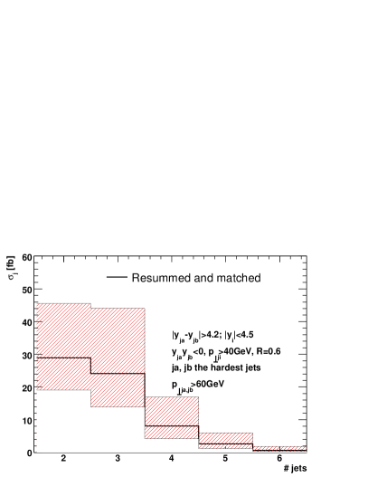
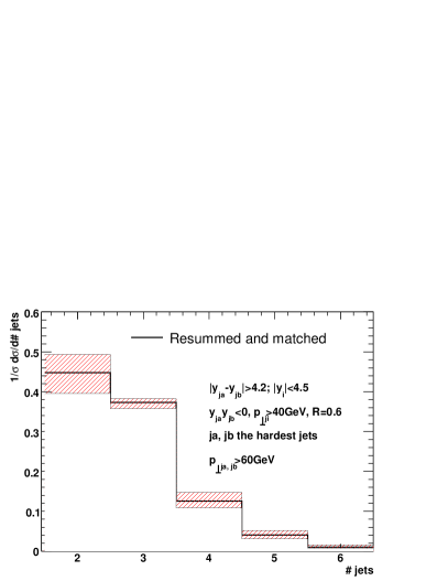
In order to better investigate the perturbative activity in-between the two hardest jets when the hard jet cuts are used, we introduce a variation of the hard jet cuts: The two hardest jets should have a transverse momentum of at least 60GeV, but the multiplicity is counted according to the number of jets with a transverse momentum above 40GeV.
The LO and cross-sections are shown in figure 19, together with the results from the modified FKL approach. We see that, just as for the cuts studied so far, the modified fixed order FKL approach describes very well the cross sections obtained with the full fixed order matrix elements. Obviously, only the three-jet cross section depends on the hardness required by the non-tagging jets. On the same figure we have plotted the average number of hard jets (GeV) against the rapidity difference between the two hardest jets (GeV) in the inclusive sample of the resummed calculation. We see that there is again a decrease in the average number of jets with increasing rapidity span, albeit milder than that of Fig.18 (right).
In the following sections which investigate the jet activity, we will also report results using this set of cuts.
5.3 Cross Sections and Jet Counts within Weak Boson Fusion Cuts
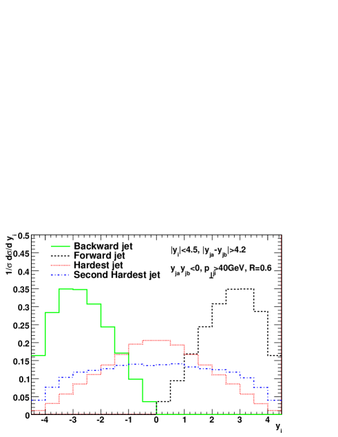
We now return to the two set of weak boson fusion cuts, differing only by the choice of jets which are required to pass the requirement on a separation in rapidity. To elucidate further the difference appearing between the “inclusive” and “hardest” choice of jet cuts, we study in Figure 20 the rapidity distribution of the most forward and backward jet, and of the hardest and next-to-hardest jet, all within the inclusive jet cuts. It is worth recalling that the events passing the cuts on the hardest jets are a sub-set of the events passing the inclusive cut. The figure demonstrates that the rapidity distribution of the hardest jet is more central than that of the next-to-hardest jet. Obviously, cuts based on the two hardest jets also being far apart in rapidity will reject many of the events with strictly more than 2 jets, which would otherwise be accepted by the inclusive cuts.
With the inclusive jet cuts and using the resummed and matched calculation, we find a total cross section of fb, where the quoted uncertainty is obtained by variation of the common factorisation and renormalisation scale by a factor of two (in the resummation, we choose to evaluate at the scale , just as in the fixed order calculations). The relative scale uncertainty is similar to the tree-level results; the scale uncertainty would be reduced if next-to-leading logarithmic corrections were taken into account. The result for the resummed cross section corresponds to an increase over the LO rate of 89%, which is only slightly larger than the K-factor of 1.7-1.8 found at NLO. The large NLO K-factor arises from the relative large 3-jet rate (only 12% less than the tree-level 2-jet rate). In the resummed calculation, the virtual and unresolved real radiation implemented by the exponentials in Eq. (3.3.5) suppress the cross section for any fixed number of partons compared to the tree-level approximation. This suppression is then counterbalanced by the sum over further real emissions.
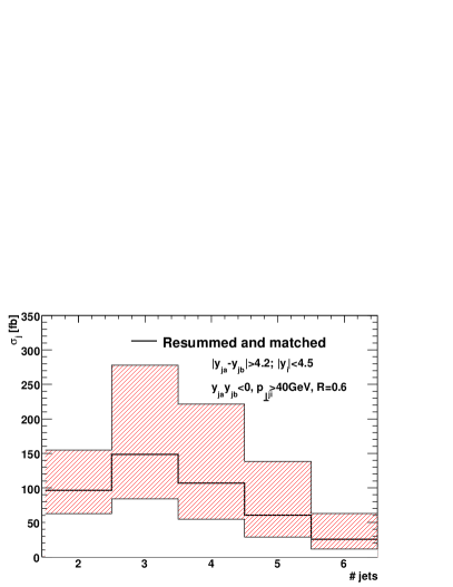
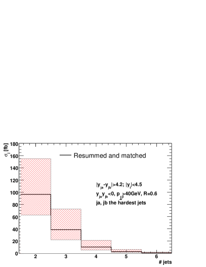
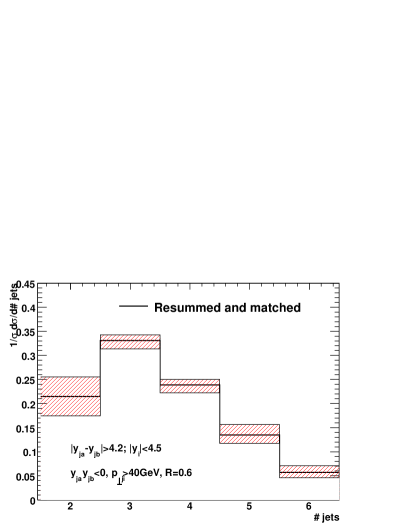
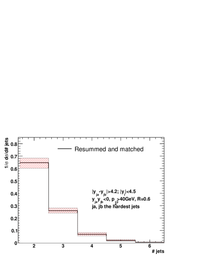
We can apply the jet finding algorithms to the resummed and matched event sample, and investigate the frequency of multiple hard jets. In Figure 21 (top left) we show the breakdown of the total cross section on the number of hard jets in each event. The red uncertainty bands arise by varying the factorisation and renormalisation scale by a factor of two. The scale variations change the overall normalisation, but has a much milder impact on the relative jet counts, as indicated in Fig. 22. We find that with the inclusive jet cuts and the chosen parameters for the jet-algorithm, the three-jet rate is larger than the two-jet rate, and from three to six jets there is an almost linear decrease in the jet rates. For the cuts on the hardest jets, the jet rates are uniformly decreasing with the jet count; the two-jet rate is more than twice as large as the three-jet rate, a pattern which continues for the higher jet rates. The jet rates are still uniformly decreasing, when furthermore the hardest jets are required to be harder than 60GeV, but all jets with a transverse momentum larger than 40GeV are counted, although obviously the higher jet counts are relatively more important than with a single jet scale.
When the two hardest jets are required to pass the cuts on rapidity separation, we find a cross section of fb, roughly 65% of the lowest order tree-level estimate reported in Section 2.1. We see a suppression compared to the LO estimate, instead of the increase of 30-40%, which is seen in the NLO calculation with the hardest cuts. As we have already discussed, the hardest cuts are very sensitive to further hard radiation beyond the 3 jets which are included in the NLO calculation. When 4 jet configurations are included, the two hardest jets are likely to be found centrally (see Fig. 20), and all such events will be rejected according to the hardest cuts. This is not taken into account in the NLO calculation, but is in the resummed calculation, which therefore results in a smaller cross section than seen at NLO. The resummed calculation can directly address the perturbative instability of the hardest cuts at the lowest fixed orders. The resummed and matched prediction for the cross section when the cuts are placed on the hardest jets, which are also required to be harder than 60GeV (see Sec. 5.2) is fb, again roughly 65% of the tree-level cross section found in Section 5.2.
The predictions for the relative number of hard jets are surprisingly stable against variations of factorisation and renormalisation scale. This is illustrated on Figures 22 for both the inclusive and hard cuts.
5.4 The Effects of a Central Rapidity Jet Veto
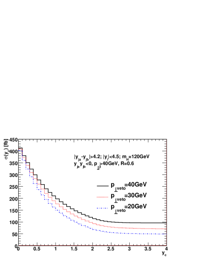
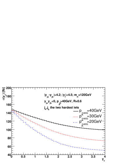
Since the weak boson fusion process has no kinematically un-suppressed colour connection between the two jets at the two lowest orders in perturbation theory, the jet activity between these is expected to be significantly lower than that of the gluon fusion process[3]. It has been suggested to use this as a further discriminator between the production mechanisms, and suppress the gluon fusion contribution by vetoing events with jets in-between the two tagged jets. Obviously, everything will depend on which two jets are chosen as the tagging ones and many other details, which necessitates a flexible generator for any study of the effects of central rapidity jet vetos; in the following we will demonstrate the effect both when the tagged jets are chosen as the ones furthest apart in rapidity, and when they are chosen as the hardest jets. We will study the cross section as a function of vetoing all further hard jets of transverse momentum greater than within a distance in rapidity from the centre of the tagged jets (always of more than 40GeV transverse momentum) of rapidity . That is, we require:
| (38) |
In the present study we will be interested only in vetoing relatively hard mini-jets[65] with transverse momentum of more than 20GeV - if the transverse momentum scale for the jet veto is significantly lower than the transverse momentum of the two tagged jets, then a sensitivity is introduced to potentially large logarithms of soft origin, see e.g. Ref. [66].
In Figure 23 (left) we show the cross section as a function of the variable introduced in Eq. (38), when the two tagged jets are those most forward and backward in rapidity (left) and when they are the hardest (right). We have included the results for and . At there is no additional cut, while for the cross section asymptotes to the two-jet cross section obtained in the resummed and matched calculation. As is lowered, more jets are resolved and more events are vetoed. For the low veto scale of and as , the cross section is reduced to 50fb or roughly a fifth of the tree-level -prediction.
Figure 23 (right) shows the results when jets are the hardest jets of the event. This asymptotes to the cross section for 2 hard jets with a softer third jet (still passing the cut on 40GeV) outside in rapidity.
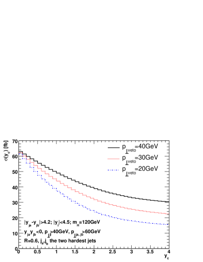
On Figure. 23 we also show the similar distribution obtained with the modified hard jet cuts discussed in Section 5.2. Again, a jet scale veto of 20GeV extended to the whole rapidity span between the two hardest jets reduces the cross section to about a fifth of the leading order estimate. Reducing the jet scale to below 20GeV would probably need a study of the interplay with the underlying event.
5.5 Azimuthal correlations
In this subsection we return to the discussion of the azimuthal correlation between two jets. In Table 3 we compare the results for (defined in Eq. (4)) using various calculations, and the two sets of cuts.
| Inclusive cuts | |
|---|---|
| LO 2-jet | |
| Resummed, -jet | |
| LO 3-jet | |
| Resummed |
| Hardest cuts | |
|---|---|
| LO 2-jet | |
| Resummed, -jet | |
| LO 3-jet | |
| Resummed |
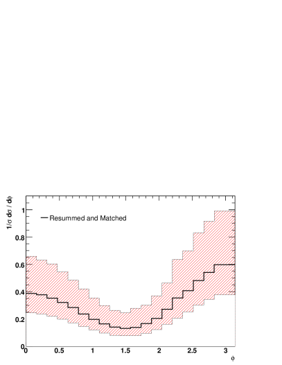
Of particular interest is the difference between the first two lines of numbers. The first () describes the result obtained in the two-jet tree-level calculation. The second () is the result obtained for events of the resummed and matched calculation, classified as containing only two hard jets, but otherwise completely inclusive. The difference is slight, and mostly due to the decorrelation caused by the additional radiation not sufficiently hard to increase the number of hard jets. These two numbers are obviously the same for the two sets of cuts, while the azimuthal correlation observed in the tree-level three-jet calculation and the fully inclusive, resummed approach depends on the choice of cuts. The value of is most stable between the different calculational procedures for the set of cuts relying on only the hardest jets in the event. This arises since there are fewer hard jets in the event samples based on the hardest cuts, which leads to stronger correlation between the hardest jets. This is illustrated in Fig. 24, which compares the distributions obtained in the resummed calculation, for both the inclusive and hard cuts.
5.6 Transverse Momentum Spectrum of the Higgs Boson
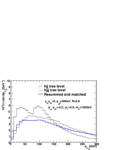
The transverse momentum spectrum of the Higgs boson when produced in association with at least two hard jets is shown in Fig. 25 for both the calculation of the tree-level , , and completely inclusive, resummed and matched procedure presented here. The spectrum is of course completely different to the one for the completely inclusive Higgs boson production (no jets required), which has previously been extensively studied in the literature, and can be obtained from the combined NNLO-NNLL calculation of Higgs boson production through gluon fusion[67]. The tree level 2 jet result has a bimodal structure, which arises from the azimuthal correlation between the two jets combined with the jet cuts. This structure disappears when extra radiation is added, giving a qualitatively different behaviour. The significant difference between the fixed-order spectra emphasises the importance of considering higher order corrections. The Higgs boson transverse momentum spectrum of the resummed calculation has a hint of a remnant from the double-hump result found at tree-level at small (GeV) transverse momenta, but is far smoother, while tending to the tree-level result for large transverse momenta.
6 Discussion
We have outlined a new technique for estimating the higher order QCD corrections in Higgs boson production via GGF. Our technique takes FKL factorisation as a starting point, as this implements hard radiation and also includes some virtual corrections, which controls the normalisation as well as cancelling singularities associated with soft gluon emissions. This is in contrast to the inclusion of collinearly enhanced (soft) radiation to hard matrix elements using a parton shower.
We define our + multiparton scattering amplitudes covering all of phase space by the FKL factorisation formula, implemented with the following requirements: (i) Use full 4-momenta for the gluon propagators; (ii) Use the Lipatov vertex as given by Eq. (10). The former implements part of the known singularity structure of higher order scattering amplitudes, whilst the latter enforces the Ward identity and positivity of the squared gluon emission vertex over all of phase space. The approach has been validated by comparison with known tree level matrix elements. As demonstrated, the approximations are generally very good, even for modest rapidity spans, which increases confidence in the reliability of the resummation procedure.
To further increase the accuracy of the approximation, we include the known tree level matrix elements for 2 and 3 final state partons using a matching prescription. In principle the matching could be extended to include higher order tree level matrix elements, although the evaluation of the tree level matrix element from standard packages become prohibitively slow. We note that matching corrections have been included in all cases where the full tree-level matrix elements have currently been used for predictions of cross sections.
We have implemented the full framework in a Monte Carlo generator, and provided example results obtained using the VBF cuts of table 1. We have thoroughly discussed differences arising from the interpretation of cuts in cases with more than 2 jets. When events are accepted if any two jets satisfy the VBF cuts of table 1, then the cross section is stable compared to the result at fixed NLO, but the impact on the correlation in azimuth between tagged jets is large. If the two hardest jets are required to also fulfil the VBF cuts, then the cross section is reduced further compared to the result at NLO, due to the possibility of additional jets, predominantly at central rapidity. However, the impact on the azimuthal correlation is much smaller. If therefore the aim is to suppress the contribution to the inclusive channel from gluon fusion, while ensuring the azimuthal correlation is modified the least from the LO estimate, then this is achieved best by tagging on the hardest jets in the event. This is, however, a result only of the effective suppression of events with central or many jets when requiring the hardest jets to pass the VBF cuts, and similar results can be achieved by use of a central rapidity jet veto.
The modified FKL formalism developed here is not unique to Higgs production but is more generally applicable to many different scattering processes, such as production of a boson with associated jets, and also purely partonic processes. These can be implemented in the existing framework, and could also be tested against existing hadron collider data.
Acknowledgments
We would like to acknowledge useful discussions with John Campbell, Keith Ellis and Gavin Salam. We are grateful to the GGI institute, Florence, where part of this work was carried out. CDW is supported by the Dutch Organisation for Fundamental Matter Research (FOM). He is grateful to the Cavendish Laboratory for hospitality, and also to Eric Laenen and Jos Vermaseren for useful discussions. This work was partly supported by MIUR under contract 2006020509004 and by the EC Marie-Curie Research Training Network “Tools and Precision Calculations for Physics Discoveries at Colliders” under contract MRTN-CT-2006-035505 .
References
- [1] G. Klamke and D. Zeppenfeld, Higgs plus two jet production via gluon fusion as a signal at the CERN LHC, hep-ph/0703202.
- [2] V. Del Duca, W. Kilgore, C. Oleari, C. Schmidt, and D. Zeppenfeld, Gluon-fusion contributions to h + 2 jet production, Nucl. Phys. B616 (2001) 367–399, [hep-ph/0108030].
- [3] Y. L. Dokshitzer, S. I. Troian, and V. A. Khoze, Collective QCD Effects in the Structure of Final Multi-Hadron States (in Russian), Sov. J. Nucl. Phys. 46 (1987) 712–719.
- [4] Y. L. Dokshitzer, V. A. Khoze, and T. Sjostrand, Rapidity gaps in Higgs production, Phys. Lett. B274 (1992) 116–121.
- [5] V. Hankele, G. Klamke, and D. Zeppenfeld, Higgs + 2 jets as a probe for CP properties, hep-ph/0605117.
- [6] T. Han, G. Valencia, and S. Willenbrock, Structure function approach to vector boson scattering in p p collisions, Phys. Rev. Lett. 69 (1992) 3274–3277, [hep-ph/9206246].
- [7] A. Djouadi, M. Spira, and P. M. Zerwas, Production of higgs bosons in proton colliders: QCD corrections, Phys. Lett. B264 (1991) 440–446.
- [8] T. Figy, C. Oleari, and D. Zeppenfeld, Next-to-leading order jet distributions for Higgs boson production via weak-boson fusion, Phys. Rev. D68 (2003) 073005, [hep-ph/0306109].
- [9] E. L. Berger and J. Campbell, Higgs boson production in weak boson fusion at next-to- leading order, Phys. Rev. D70 (2004) 073011, [hep-ph/0403194].
- [10] T. Figy, V. Hankele, and D. Zeppenfeld, Next-to-leading order QCD corrections to Higgs plus three jet production in vector-boson fusion, JHEP 02 (2008) 076, [0710.5621].
- [11] R. V. Harlander, J. Vollinga, and M. M. Weber, Gluon-Induced Weak Boson Fusion, Phys. Rev. D77 (2008) 053010, [0801.3355].
- [12] M. Ciccolini, A. Denner, and S. Dittmaier, Strong and electroweak corrections to the production of Higgs+2jets via weak interactions at the LHC, Phys. Rev. Lett. 99 (2007) 161803, [0707.0381].
- [13] M. Ciccolini, A. Denner, and S. Dittmaier, Electroweak and QCD corrections to Higgs production via vector-boson fusion at the LHC, Phys. Rev. D77 (2008) 013002, [0710.4749].
- [14] J. R. Andersen and J. M. Smillie, QCD and electroweak interference in Higgs production by gauge boson fusion, Phys. Rev. D75 (2007) 037301, [hep-ph/0611281].
- [15] J. R. Andersen, T. Binoth, G. Heinrich, and J. M. Smillie, Loop induced interference effects in Higgs Boson plus two jet production at the LHC, JHEP 02 (2008) 057, [0709.3513].
- [16] A. Bredenstein, K. Hagiwara, and B. Jager, Mixed QCD-electroweak contributions to Higgs-plus-dijet production at the LHC, Phys. Rev. D77 (2008) 073004, [0801.4231].
- [17] V. Del Duca, W. Kilgore, C. Oleari, C. Schmidt, and D. Zeppenfeld, H + 2 jets via gluon fusion, Phys. Rev. Lett. 87 (2001) 122001, [hep-ph/0105129].
- [18] R. P. Kauffman, S. V. Desai, and D. Risal, Production of a higgs boson plus two jets in hadronic collisions, Phys. Rev. D55 (1997) 4005–4015, [hep-ph/9610541].
- [19] F. Wilczek, Decays of Heavy Vector Mesons Into Higgs Particles, Phys. Rev. Lett. 39 (1977) 1304.
- [20] S. Dawson, Radiative corrections to higgs boson production, Nucl. Phys. B359 (1991) 283–300.
- [21] V. Del Duca, W. Kilgore, C. Oleari, C. R. Schmidt, and D. Zeppenfeld, Kinematical limits on Higgs boson production via gluon fusion in association with jets, Phys. Rev. D67 (2003) 073003, [hep-ph/0301013].
- [22] S. Marzani, R. D. Ball, V. Del Duca, S. Forte, and A. Vicini, Higgs production via gluon-gluon fusion with finite top mass beyond next-to-leading order, Nucl. Phys. B800 (2008) 127–145, [0801.2544].
- [23] V. Del Duca, A. Frizzo, and F. Maltoni, Higgs boson production in association with three jets, JHEP 05 (2004) 064, [hep-ph/0404013].
- [24] L. J. Dixon, E. W. N. Glover, and V. V. Khoze, MHV rules for Higgs plus multi-gluon amplitudes, JHEP 12 (2004) 015, [hep-th/0411092].
- [25] S. D. Badger, E. W. N. Glover, and V. V. Khoze, MHV rules for Higgs plus multi-parton amplitudes, JHEP 03 (2005) 023, [hep-th/0412275].
- [26] R. K. Ellis, W. T. Giele, and G. Zanderighi, Virtual qcd corrections to higgs boson plus four parton processes, Phys. Rev. D72 (2005) 054018, [hep-ph/0506196].
- [27] J. M. Campbell, R. K. Ellis, and G. Zanderighi, Next-to-leading order higgs + 2 jet production via gluon fusion, JHEP 10 (2006) 028, [hep-ph/0608194].
- [28] V. Del Duca et al., Monte Carlo studies of the jet activity in higgs + 2jet events, JHEP 10 (2006) 016, [hep-ph/0608158].
- [29] V. S. Fadin, E. A. Kuraev, and L. N. Lipatov, On the Pomeranchuk singularity in asymptotically free theories, Phys. Lett. B60 (1975) 50–52.
- [30] E. A. Kuraev, L. N. Lipatov, and V. S. Fadin, Multi - Reggeon processes in the Yang-Mills theory, Sov. Phys. JETP 44 (1976) 443–450.
- [31] E. A. Kuraev, L. N. Lipatov, and V. S. Fadin, The Pomeranchuk singularity in nonabelian gauge theories, Sov. Phys. JETP 45 (1977) 199–204.
- [32] I. I. Balitsky and L. N. Lipatov, The Pomeranchuk singularity in quantum chromodynamics, Sov. J. Nucl. Phys. 28 (1978) 822–829.
- [33] S. Dawson and R. Kauffman, QCD corrections to Higgs boson production: nonleading terms in the heavy quark limit, Phys. Rev. D49 (1994) 2298–2309, [hep-ph/9310281].
- [34] A. D. Martin, R. G. Roberts, W. J. Stirling, and R. S. Thorne, Physical gluons and high-e(t) jets, Phys. Lett. B604 (2004) 61–68, [hep-ph/0410230].
- [35] J. Alwall et al., MadGraph/MadEvent v4: The new web generation, JHEP 09 (2007) 028, [arXiv:0706.2334 [hep-ph]].
- [36] M. Cacciari and G. P. Salam, Dispelling the n**3 myth for the k(t) jet-finder, Phys. Lett. B641 (2006) 57–61, [hep-ph/0512210].
- [37] T. Regge, Introduction to complex orbital momenta, Nuovo Cim. 14 (1959) 951.
- [38] T. Regge, Bound states, shadow states and Mandelstam representation, Nuovo Cim. 18 (1960) 947–956.
- [39] R. C. Brower, C. E. DeTar, and J. H. Weis, Regge Theory for Multiparticle Amplitudes, Phys. Rept. 14 (1974) 257.
- [40] P. D. B. Collins, An Introduction to Regge Theory and High-Energy Physics, . Cambridge 1977, 445p.
- [41] R. J. Eden, P. V. Landshoff, D. I. Olive, and J. C. Polkinghorne, The analytic -matrix, . Cambridge 1966, 295p.
- [42] I. I. Balitsky, L. N. Lipatov, and V. S. Fadin, REGGE PROCESSES IN NONABELIAN GAUGE THEORIES. (IN RUSSIAN), . In *Leningrad 1979, Proceedings, Physics Of Elementary Particles*, Leningrad 1979, 109-149.
- [43] V. S. Fadin, R. Fiore, M. G. Kozlov, and A. V. Reznichenko, Proof of the multi-Regge form of QCD amplitudes with gluon exchanges in the NLA, hep-ph/0602006.
- [44] V. Del Duca, An introduction to the perturbative QCD pomeron and to jet physics at large rapidities, http://arXiv.org/abs/hep-ph/9503226.
- [45] V. S. Fadin, BFKL news, hep-ph/9807528.
- [46] J. R. Andersen and C. D. White, A New Framework for Multijet Predictions and its application to Higgs Boson production at the LHC, 0802.2858.
- [47] B. L. Combridge and C. J. Maxwell, Untangling large p(t) hadronic reactions, Nucl. Phys. B239 (1984) 429.
- [48] A. V. Bogdan and V. S. Fadin, A proof of the reggeized form of amplitudes with quark exchanges, Nucl. Phys. B740 (2006) 36–57, [hep-ph/0601117].
- [49] J. R. Andersen, On the role of NLL corrections and energy conservation in the high energy evolution of QCD, Phys. Lett. B639 (2006) 290–293, [hep-ph/0602182].
- [50] L. H. Orr and W. J. Stirling, Dijet production at hadron hadron colliders in the BFKL approach, Phys. Rev. D56 (1997) 5875–5884, [hep-ph/9706529].
- [51] C. R. Schmidt, A Monte Carlo solution to the BFKL equation, Phys. Rev. Lett. 78 (1997) 4531–4535, [hep-ph/9612454].
- [52] J. R. Andersen, V. Del Duca, S. Frixione, C. R. Schmidt, and W. J. Stirling, Mueller-Navelet jets at hadron colliders, JHEP 02 (2001) 007, [http://arXiv.org/abs/hep-ph/0101180].
- [53] J. Bartels and H. Lotter, A Note on the BFKL pomeron and the ’hot spot’ cross- section, Phys. Lett. B309 (1993) 400–408.
- [54] M. Ciafaloni, Coherence effects in initial jets at small q**2 / s, Nucl. Phys. B296 (1988) 49.
- [55] B. Andersson, G. Gustafson, and J. Samuelsson, The linked dipole chain model for DIS, Nucl. Phys. B467 (1996) 443–478.
- [56] S. Catani, F. Fiorani, and G. Marchesini, Small x behavior of initial state radiation in perturbative qcd, Nucl. Phys. B336 (1990) 18.
- [57] S. Catani, F. Fiorani, and G. Marchesini, Qcd coherence in initial state radiation, Phys. Lett. B234 (1990) 339.
- [58] J. Kwiecinski, A. D. Martin, and P. J. Sutton, Constraints on gluon evolution at small x, Z. Phys. C71 (1996) 585–594, [hep-ph/9602320].
- [59] J. Kwiecinski, C. A. M. Lewis, and A. D. Martin, Observable jets from the BFKL chain, Phys. Rev. D54 (1996) 6664–6673, [hep-ph/9606375].
- [60] J. R. Andersen and A. Sabio Vera, Solving the BFKL equation in the next-to-leading approximation, Phys. Lett. B567 (2003) 116–124, [hep-ph/0305236].
- [61] J. R. Andersen and A. Sabio Vera, The gluon green’s function in the BFKL approach at next-to-leading logarithmic accuracy, Nucl. Phys. B679 (2004) 345–362, [hep-ph/0309331].
- [62] J. R. Andersen, The quark-antiquark contribution to the fully exclusive BFKL evolution at NLL accuracy, hep-ph/0611011.
- [63] J. R. Andersen, A closer look at the analysis of NLL BFKL, AIP Conf. Proc. 792 (2005) 726–732, [hep-ph/0507215].
- [64] S. Catani, L. Trentadue, G. Turnock, and B. R. Webber, Resummation of large logarithms in e+ e- event shape distributions, Nucl. Phys. B407 (1993) 3–42.
- [65] V. D. Barger, R. J. N. Phillips, and D. Zeppenfeld, Mini - jet veto: A tool for the heavy Higgs search at the LHC, Phys. Lett. B346 (1995) 106–114, [http://arXiv.org/abs/hep-ph/9412276].
- [66] J. R. Forshaw and M. Sjödahl, Soft gluons in Higgs plus two jet production, JHEP 09 (2007) 119, [0705.1504].
- [67] G. Bozzi, S. Catani, D. de Florian, and M. Grazzini, Higgs boson production at the LHC: transverse-momentum resummation and rapidity dependence, Nucl. Phys. B791 (2008) 1–19, [0705.3887].