Studying Geometric Graph Properties of Road Networks
Through an Algorithmic Lens

Abstract

This paper studies the geometric graph properties of road networks from an algorithmic perspective, focusing on empirical studies that yield useful properties of road networks and how these properties can be exploited in the design of fast algorithms. Unlike previous approaches, our study is not based on the assumption that road networks are planar graphs. Indeed, based on experiments we have performed on the road networks of the 50 United States and District of Columbia, we provide strong empirical evidence that road networks are quite non-planar. Our approach instead is directed at finding algorithmically-motivated properties of road networks as non-planar geometric graphs, focusing on alternative properties of road networks that can still lead to efficient algorithms for such problems as shortest paths and Voronoi diagrams. In particular, we study road networks as multiscale-dispersed graphs, which is a concept we formalize in terms of disk neighborhood systems. This approach allows us to develop fast algorithms for road networks without making any additional assumptions about the distribution of edge weights.

Keywords: road networks, disk neighborhood systems, circle arrangements, multiscale-dispersed graphs, shortest paths, Voronoi diagrams, algorithmic lens.

1 Introduction

With the advent of online mapping systems, including proprietary systems like Google Maps and Mapquest, and open-source projects like http://wiki.openstreetmap.org/, there is an increased interest in studying road networks as natural artifacts. Indeed, the Ninth DIMACS Implementation Challenge, from 2006, was dedicated to the algorithmic study of road networks from the perspective of methods for solving shortest path problems on road networks. (See Figure 1 for an example extracted from this data.)

Figure 1: A portion of the road network from the U.S. Census 2000 TIGER/Line files. This example illustrates the road network for Anchorage, Alaska, which consists of over 9,000 vertices and 23,000 edges.

Road networks provide an interesting domain of study, from an algorithmic perspective, as they combine geographic and graph-theoretic information in one structure. In particular, road networks can be viewed as instances of geometric graphs [37], that is, graphs in which each vertex is associated with a unique point in ${\bf R}^{2}$ and each edge is associated with a simple curve joining the points associated with its end vertices. In the case of a road network, we create a vertex for every road intersection or major jog and we create an edge for every road segment that joins two such points. In addition, road networks contain geographic information, in that vertices are usually labeled with their (GPS) longitude and latitude coordinates and edges are labeled with their length. These basic data attributes of road networks, together with the fundamental anthropological nature of the way these networks encapsulate the way that societies organize themselves, make road networks unique data objects. Therefore, following similar studies of natural artifacts through the algorithmic lens (e.g., see [1, 4, 11, 10, 13, 38, 45]), we are interested in this paper in the study of algorithmically motivated properties of road networks as geometric graphs.

1.1 Geometric Graph Properties of Road Networks

Because roads are built on the surface of the Earth, which as a first-order approximation is a sphere, it is tempting to view them as plane graphs [15, 20, 44], that is, graphs that are drawn on the surface of a sphere without edge crossings. Indeed, some statistics commonly used to characterize road networks only make sense for planar graphs (e.g., see [12]). For example, the Alpha index for a road network with $n$ vertices is the ratio of the number of internal fundamental cycles to $2n-5$, which is called “the maximum possible,” but this maximum doesn’t hold for non-planar graphs. Likewise, the Gamma index is the ratio of the number of edges in a road network to $3n-6$, which is another “maximum possible” that doesn’t hold for non-planar graphs. (The values $2n-5$ and $3n-6$ come from Euler’s formula for planar graphs.) Such statistics are often used to measure the density of road networks, and, as standardized numbers, they probably suffice for this purpose, but they may also give the false impression that road networks are plane graphs.

Anyone who has seen an expressway underpass has firsthand experience of a counter-example to the planarity of road networks. Of course, if such edge crossings were rare, it would probably still be okay to think of road networks as plane graphs or “almost plane” graphs. In fact, as we show in the experimental results of this paper, real-world road networks can have many edge crossings. For example, the road network for California—with its extensive freeway system—has almost 6,000 edge crossings! Thus, the main goal of this paper is to exploit an alternative geometric characterization of road networks that reflects their non-planar nature. Additionally, we wish to avoid making any assumptions about the distribution of edge weights, because it is important in many transportation planning problems to use artificial weights that do not reflect the geometry of the input and that may vary from user to user [16].

The approach we study in this paper is based on characterizing road networks as subgraphs of disk intersection graphs, in a way that takes advantage of their bounded-depth fractal nature [7]. In particular, we exploit the manner in which road networks reflect the way populations naturally create geographic features that are well-separated at multiple scales in a self-similar fashion. We introduce a formalism that characterizes road networks as multiscale-dispersed graphs, which is itself based on viewing road networks as subgraphs of disk intersection graphs.

A disk intersection graph is defined from a collection $S$ of disks in ${\bf R}^{2}$ by creating a vertex for every disk in $S$ and defining an edge for every pair of intersecting disks in $S$. Disk intersection graphs include the planar graphs, since, by a beautiful result of Koebe [29], every planar graph can be represented as the intersection graph of a set of disks that intersect only at their boundaries. Moreover, by a result of Mohar [36], such embeddings can be constructed in polynomial time. A set $S$ of disks in the plane defines a $k$-ply neighborhood system if, for any point $p\in{\bf R}^{2}$, the number of disks from $S$ containing $p$ is at most $k$. Thus, the collection of “kissing” disks used in the representation of Koebe [29] for a planar graph defines a $2$-ply neighborhood system.

The natural way to define a disk neighborhood system from a road network $G$ is to center a disk at each vertex $v$ in $G$ and define its radius to be half the length of the longest edge incident to $v$ in $G$. The intersection graph of such a disk neighborhood system is guaranteed to contain $G$ as a subgraph. Thus, we define this as the natural disk neighborhood system determined by the road network $G$, and we use this notion throughout this paper. (See Figure 2.)

Figure 2: The natural disk neighborhood system for the road network of Anchorage, Alaska, which was presented in Figure 1.

We exploit this characterization by showing that it allows us to utilize a technique used in many fast algorithms for planar graphs—the the existence of efficient methods for finding small-sized separators [30]. These are small sets of vertices whose removal separates the graph into two subgraphs of roughly equal size. Interestingly, like planar graphs, $k$-ply neighborhood systems of disks have small-sized separators (e.g., see [3, 34, 35, 42]). In order to handle the intricacies of road networks, the natural disk neighborhood systems of which may not be $k$-ply, we generalize these results by showing that small separators exist for a larger related class of graphs. Moreover, there exist algorithms for finding good separators in $k$-ply neighborhood systems and our generalizations of them, and these algorithms can be used to construct efficient algorithms for such graphs, as we show.

Additional experiments we provide in this paper justify the claim that real-world road networks have the properties mentioned above. Moreover, we show that our approach leads to improved algorithms and data structures for dealing with real-world road networks, including shortest paths and Voronoi diagrams. In general, we desire comparison-based algorithms that require no additional assumptions regarding the distribution of edge weights, so that our algorithms can apply to a wide variety of possible edge weights, including (non-metric) combinations of distance, travel time, toll charges, and subjective scores rating safety and scenic interest.

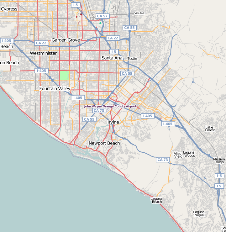
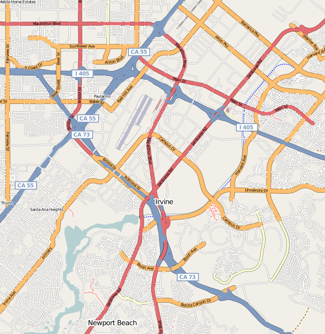
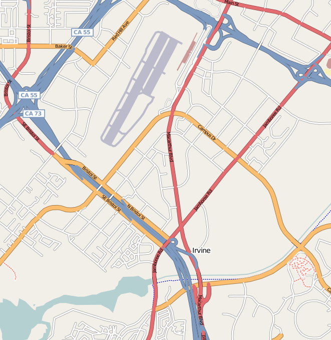
Figure 3: The multiscale dispersion of real-world maps. These three images show various scales of maps of Irvine, California. Images are from http://wiki.openstreetmap.org/, under the Creative Commons attribution-share alike license.

1.2 Previous Related Work

There has been considerable work in the transportation literature on studies of the properties of road networks (e.g., see [12]), including analyses based on the Alpha and Gamma indices. As mentioned above, however, much of this work implicitly assumes that road networks are planar.

In the algorithms community, there has been considerable prior work on shortest path algorithms for road networks and Euclidean graphs (e.g., see [23, 27, 28, 40, 41, 46] and the program for the Ninth DIMACS Implementation Challenge). This prior work on road network algorithms takes a decidedly different approach than we take in this paper, however, in that this prior work focuses on using special properties of the edge weights that do not hold in the comparison model, whereas we study road networks as a graph family and desire properties that would result in efficient algorithms in the comparison model.

One of the main ingredients we use in our algorithms is the existence of small separators in certain graph families (e.g., see [30, 33]). Previous work on separators includes the seminal contribution of Lipton and Tarjan [30], who showed that $O(\sqrt{n})$-sized separators exist for $n$-vertex planar graphs and these can be computed in $O(n)$ time. Goodrich [24] shows that recursive $O(\sqrt{n})$-separator decompositions can be constructed for planar graphs in $O(n)$ time. A related concept is that of geometric separators, which use geometric objects to define separators in geometric graphs (e.g., see [3, 34, 35, 42]), for which Eppstein et al. [18] provide a linear-time construction algorithm, which translates into an $O(n\log n)$-time recursive separator decomposition algorithm.

The specific algorithmic problems we study are well-known in the general algorithms and computational geometry literatures. For general graphs with $n$ vertices and $m$ edges, excellent work can be found on efficient algorithms in the comparison model, including single-source shortest paths [14, 25, 39], which takes $O(n\log n+m)$ time [21], and Voronoi diagrams [5, 6], whose graph-theoretic version can be constructed in $O(n\log n+m)$ time [19, 31]. Note that none of these algorithms run in linear time, even for planar graphs. Nevertheless, linear-time algorithms for planar graphs are known for single-source shortest paths [26], which unfortunately do not immediately translate into linear-time algorithms for road networks. In addition, there are a number of efficient shortest-path algorithms that make assumptions about edge weights [22, 23, 32, 43]; hence, are not applicable in the comparison model. Eppstein et al. [17] show how to find all the edge interesections in an $n$-vertex straight-line geometric graph in $O(n+k\log^{(c)}n)$ expected time, where $k$ is the number of pairwise edge intersections and $c$ is any fixed constant, and they show how this can be combined with the method of Goodrich [24] to construct a recursive $O(\sqrt{n})$-separator decomposition for such a graph in $O(n)$ time if $k$ is $O(n/\log^{(c)}n)$. There method does not result in a geometric separator decomposition, however, as our approach in this paper does.

1.3 Our Results

In this paper, we study properties of road networks that can be exploited in efficient algorithms for such networks. In particular, we view road networks as a special class of non-planar geometric graphs and we show how to design efficient algorithms for them that are based on their characterization as embedded graphs that that have well-dispersed vertices and edges. We use the automatic multiscale nature of disk neighborhoods to capture the property that the spatial distribution of edges is similar at multiple scales, like fractals, except that this recursive self-similarity has a bounded depth [7]. (See Figure 3.)

We provide experimental evidence that debunks the belief that road networks are plane graphs or even “almost planar.” Instead, we provide empirical evidence that real-world road networks have natural disk neighborhood systems that are subgraphs of $k$-ply disk intersection graphs (with a small number of exceptions), for constant $k$. That is, road networks are multiscale-dispersed graphs. Our analysis uses the U.S. TIGER/Line road network database, as provided by the Ninth DIMACS Implementation Challenge, which is comprised of over 24 million vertices and 29 million edges.

Viewing road networks as multiscale-dispersed graphs allows us to prove that these networks have small geometric separators, which can be found quickly. Furthermore, we show how to use recursive separator decompositions for road networks in the design of fast shortest path and Voronoi diagram algorithms for road networks. We also provide a fast algorithm for constructing the arrangement of circles in a natural disk neighborhood system, using additional algorithmic properties of road networks, which we justify empirically. Thus, we justify the claim that viewing road networks through the algorithmic lens can lead to the discovery of properties of these networks that result in algorithms that run faster than algorithms that would simply view these networks as standard graphs.

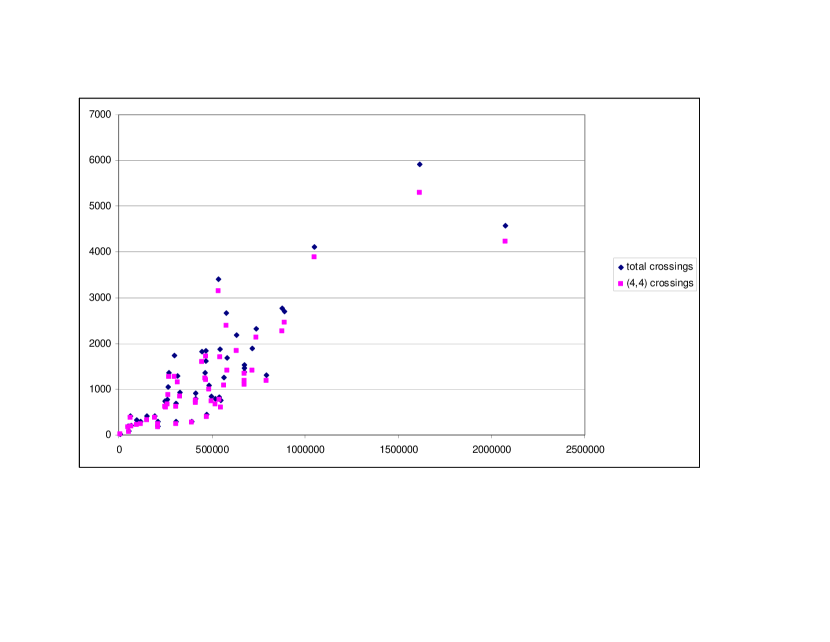
Figure 4: A scatter plot of the number of edge crossings for TIGER/Line road networks, indexed by network size, listed as both total number of crossings and number of crossings between pairs of edges such that both are in the highest level of the road network hierarchy.

2 Non-Planarity

As noted above, every road network is a graph $G=(V,E)$, having a set, $V$, of $n$ vertices, defined by road junctions and on/off ramps, and a set, $E$, of $m$ edges, defined by the uninterrupted pieces of roads, highways, and expressways between such vertices. Since the number of roads that meet at a single junction cannot be arbitrarily large, road networks have bounded degree. Thus, the number, $m$, of edges in a road network is $O(n)$. For this reason, we will focus on $n$ as the key factor defining the “size” of a road network.

As mentioned above, road networks are geometric graphs [37]. That is, they are “drawn” on a surface, so that vertices are placed at distinct points and edges correspond to simple curves, which in this paper we assume are straight line segments. In addition, the edges incident to each edge are given in a specific order, e.g., clockwise or counter-clockwise. In addition to this ordering information, road networks also have geographic information: namely, each vertex in a road network is given two-dimensional GPS coordinates, which in turn imply the line segments defined by edges. If none of these segments cross each other, and the surface is a sphere or a plane, then the embedding is said to be a plane graph [15, 20, 44]. Graphs that can be drawn as plane graphs are called planar graphs.

As mentioned above, much previous work has been done that studies road networks as plane graphs. The first set of experimental results we share in this paper show that in the road networks of the 50 United States and District of Columbia are not plane graphs. Indeed, these experiments show that none of these graphs are even “almost planar” graphs. In actuality, however, every road network in the TIGER/Line database contains multiple edge crossings, as shown in the plot of Figure 4. Indeed, some road networks have thousands of crossings. In general, the road networks tested have a number of crossings that appears to be proportional to $\sqrt{n}$, where $n$ is the number of vertices.

There is a refinement of the belief that road-networks are plane graphs, which deals with the hierarchal nature of road networks. In particular, the edges in most road-network databases are categorized according to a discrete hierarchy, with European road networks usually having 13 types of road segments and U.S. networks usually having 4, which correspond roughly to U.S. highways, state highways, major roads, and local roads. A refined belief could be that road networks are planar at each level of hierarchy, given that these hierarchies are intended to capture the various scales of “resolution” in road networks. Unfortunately, this belief is also unsupported by the data, as a refined analysis of the crossing counting data shows that most of the crossings are actually between edges in the same level of the hierarchy. Indeed, Figure 4 shows that the vast majority of crossings are between pairs of edges in the highest level of the hierarchy (level 4), which is intended for local roads.

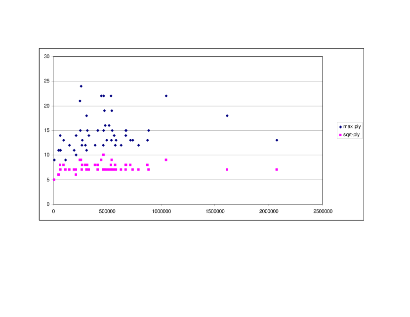
Figure 5: A scatter plot of the maximum ply of vertices in each road network and a scatter plot of the $\lfloor\sqrt{n}\rfloor$-th largest vertex ply, both indexed by network size.

The take-away message from the above analysis is that if we view road networks as being geometric graphs drawn on a sphere, then they have many edge crossings. In particular, if we have an $n$-vertex road network, then there will typically be $\Theta(\sqrt{n})$ edge crossings when all those segments are projected on the surface of a sphere using their GPS coordinates. Of course, road segments are not projected on the surface of a sphere and they don’t actually intersect; hence, roads that have apparent crossings are the result of overpasses, tunnels, data errors, or representational imprecisions.

A natural question, of course, is to ask why the number of edge crossings in road networks is proportional to $\sqrt{n}$. One possible explanation comes by way of analogy. Imagine an idealized city, which we will call Gotham City, that has a road network that, at its finest grain of detail, consists of an orthogonal grid of roads, like downtown Manhattan. Suppose at the next coarser grain of detail, Gotham City has an expressway network built on top of its fine-grain road grid, with the number of expressways being constant. Since expressways are built for fast transport, they are unlikely to have large zig-zags or consist of large spiral segments. Instead, they would be built to cut straight through Gotham City. Since any straight segment cutting through an orthogonal grid will intersect $O(\sqrt{n})$, this implies that the number of edge crossings in Gotham City’s road network is $O(\sqrt{n})$. Likewise, a random Delaunay triangulation (which is a natural way of triangulating a set of points), defined on $n$ points, will have a similar property—in that any line will intersect an expected $O(\sqrt{n})$ of segments of such a triangulation [8]. A similar phenomenon, occurring at a grander scale, could be the motivating reason why real-world road networks tend to have $O(\sqrt{n})$ edge crossings, with the existence of noisy data (which tends to increase the number of edge crossings) offsetting the fact that expressways and large highways are built in a way that tries to avoid needless overpasses (which tends to reduce the number of edge crossings). In any case, we can use the non-planarity of road networks to motivate an alternative characterization of road networks, as seen through an algorithmic lens.

3 Disk Neighborhood Systems

We define a neighborhood system $S$ of $n$ disks in the plane to be an $f(n)$-exceptional $k$-ply system if there is a function, $f(n)$, such that there exists a subset $T$ of $f(n)$ disks in $S$ so that $S-T$ forms a $k$-ply neighborhood system and every disk in $T$ intersects at most $f(n)$ disks in $S$. Intuitively, the disks in $T$ are the “exceptions that prove the rule” that $S$ is, for the most part, a $k$-ply neighborhood system. Given a graph $G$ with $n$ vertices that is embedded in ${\bf R}^{2}$, we say that $G$ is a multiscale-dispersed graph if its natural disk neighborhood system is an $O(\sqrt{n})$-exceptional $O(1)$-ply system. As mentioned above, the motivation for the constant-ply part of this definition is that the edges and vertices of road networks tend to be well-spaced, in a bounded-depth fractal way [7]. By including disks of widely varying sizes, our definition allows the simultaneous treatment of road network features of widely varying scales, but (with the removal of the exceptional disks) the remaining disks must be well dispersed in order to achieve the $k$-ply property.

The choice of an $O(\sqrt{n})$ asymptotic growth rate for the exceptional part of the definition comes from the possible existence of overlapping large disks. Such large disks are troublesome with respect to our desire for having all disks define a constant-ply disk neighborhood system if these large disks all overlap a dense urban region. Of course, large disks in a natural disk neighborhood system are defined by the long roads. Moreover, it is not unusual for long roads to lead to dense urban regions, as in the classic “all roads lead to Rome” phenomenon. Nevertheless, it is natural for urban areas to have shapes with bounded aspect ratios (e.g., see [7]), since inhabitants of such regions naturally like to be close to each other. Thus, the map footprints of urban areas tend to have perimeters that are proportional to the square root of their areas. Thus, if a dense city, like Gotham City, has $O(n)$ internal edges, it will have $O(\sqrt{n})$ boundary edges. But this necessarily bounds the number of long incoming roads to be $O(\sqrt{n})$.

Our definitions are not simply motivated by geographical arguments, however. In Figure 5 we show a scatter plot from experiments that support the claim that the maximum ply of natural disk neighborhood systems for real-world $n$-vertex road networks is higher than the $\lfloor\sqrt{n}\rfloor$-th largest vertex ply, which itself is a small constant. In particular, even for small road networks, it shows that the largest circle-center ply can be more than $20$, whereas all the $\lfloor\sqrt{n}\rfloor$-th largest vertex plies are at most $10$. Using an argument similar to that used in the proof of the following lemma (1), we can show that the maximum ply of a disk neighborhood system is within a constant factor of the maximum ply of the centers of the disks, that is, the vertices of our road networks. Thus, this empirical analysis supports the claim that the natural disk neighborhood systems of real-world road networks are $O(\sqrt{n})$-exceptional $O(1)$-ply systems. We explore one implication of the multiscale-dispersed graph property in the following lemma.

Lemma 1

If $G$ is an $n$-vertex multiscale-dispersed graph, then the number of pairs of intersecting disks in $G$’s natural disk neighborhood system is $O(n)$.

Proof: Since $G$ is a multiscale-dispersed graph, its natural disk neighborhood system, $S$, is an $O(\sqrt{n})$-exceptional $O(1)$-ply neighborhood system. Let $T$ denote the subset of $S$ of at most $O(\sqrt{n})$ disks in $S$ such that each disk in $T$ intersects at most $O(\sqrt{n})$ other disks in $S$. Clearly, the number of pairs of intersecting disks in $S$ such that one of them is in $T$ is $O(n)$. Thus, we have only to count the number of pairs of intersecting disks such that both are in $S-T$, which we could do using a lemma (3.3.2) of Miller et al. [35], but we include a counting argument here for completeness and because it leads to a better constant factor. Let $k\in O(1)$ denote the ply of the disks in $S-T$, and let us consider the two cases for a pair of intersecting disks $c$ and $d$ in $S-T$:

1. One of $c$ and $d$ contains the center of the other. In this case, we charge this intersection to a disk in $\{c,d\}$ whose center is contained inside the other disk. Let us call this a “containment” charge.

2. Neither $c$ nor $d$ contains the center of the other. In this case, we charge this intersection to the smaller of the disks $c$ and $d$. Let us call this a “tall” charge.

To complete the proof, we need only account for these two types of charges in turn. First, note that, since $S-T$ is a $k$-ply system, each disk can receive at most $k\in O(1)$ containment charges (for at most $k$ disks can contain the center of any disk). So we have only to account for the number of tall charges a disk $c$ can receive. Suppose $d$ is a disk larger than $c$ that intersects $c$ and does not contain $c$’s center. There are at most $k$ other disks that can contain $d$’s center and also intersect $c$. Thus, the total number of tall charges $c$ can receive is at most $k$ times the number of disks larger than $c$ that do not contain each other’s centers and which intersect $c$. If we order the centers of these disks around $c$, then each consecutive pair of centers defines a triangle whose side oppose $c$ is largest; hence, its angle at $c$ is largest. Therefore, there can be at most $6$ such disks, which implies that the number of tall charges $c$ can receive is at most $6k$, which is $O(1)$.  

Corollary 2

The combinatorial complexity of the arrangement, ${\cal A}(S)$, of circles determined by the natural disk neighborhood system, $S$, of a multiscale-dispersed graph is $O(n)$.

Proof: Every intersecting pair of disks in $S$ determines at most two vertices in ${\cal A}(S)$. Thus, by Lemma 1, the combinatorial complexity of ${\cal A}(S)$ is $O(n)$.  

We have shown empirically above that an $n$-vertex road network is a geometric graph having $\Theta(\sqrt{n})$ edge crossings. Interestingly, our characterization of road networks as bounded-degree multiscale-dispersed graphs can be used to imply an alternative upper bound on the number of crossings among the edges of a road network. This linear upper bound is not as strong as the above characterization, but it is nevertheless much better than the quadratic bound that would be expected from a random geometric graph.

Lemma 3

Let $G$ be an $n$-vertex multiscale-dispersed graph with bounded degree. Then the number of pairs of edges of $G$ that cross in ${\bf R}^{2}$ is $O(n)$.

Proof: Let $S$ be the natural disk neighborhood system for $G$. Suppose two edges $e_{1}=(u,v)$ and $e_{2}=(w,z)$ in $G$ cross in ${\bf R}^{2}$ at some point $p$ (note: we do not assume these edges are straight lines). Let $d_{e_{x}}(p,\nu)$ denote the distance from $p$ to the endvertex $\nu$ along the edge (curve) $e_{x}$. Then, without loss of generality, $d_{e_{1}}(p,u)\leq d_{e_{1}}(p,v)$ and $d_{e_{2}}(p,w)\leq d_{e_{2}}(p,z)$. Note that, by the definition of a natural disk neighborhood system, the radius of $u$’s disk is at least $d_{e_{1}}(p,u)$ and the radius of $w$’s disk is at least $d_{e_{2}}(p,w)$; hence, $u$’s disk intersects $w$’s disk. Let us therefore charge this pair of vertices for this edge crossing. Note that, since $G$ has bounded degree, this pair of vertices can be charged at most $O(1)$ times in this way (specifically, each such pair can be charged at most $O({\rm degree}(G)^{2})$ times). Furthermore, by Lemma 1, there are only $O(n)$ pairs of intersecting disks in $S$. Therefore, the number of pairs of edges of $G$ that cross in ${\bf R}^{2}$ is $O(n)$.  

Thus, our characterization allows for an even larger number of intersections than occur in practice. More importantly, our characterization allows for us to construct efficient algorithms for important problems involving road networks.

4 Separator Decomposition and Its Applications

In some applications, we desire algorithms for small-sized separators. Given a graph $G$, an $f(n)$-separator for $G$ is a set of $f(n)$ vertices whose removal from $G$ results in $G$ being subdivided into two subgraphs having at most $\delta n$ vertices each [24, 30, 33], for some fixed constant $0<\delta<1$.

We may alternatively desire algorithms for small-sized geometric separators, which are defined for disk systems. Given a collection of disks $S$ in ${\bf R}^{2}$, a Jordan curve $f(n)$-separator for $S$ is a Jordan curve $J$ that intersects at most $f(n)$ disks in $S$ so that at most $\delta n$ disks are either inside the interior or exterior of $J$, for some fixed constant $0<\delta<1$. Ideally, $J$ should be a simple curve, like a circle, and indeed, Eppstein et al. [18] show that $k$-ply disk neighborhood systems have linear-time computable circle $O(\sqrt{n})$-separators for $\delta=3/4$, where $k$ is a constant. We immediately have the following:

Theorem 4

Suppose we are given a set $S$ that is an $O(\sqrt{n})$-exceptional $O(1)$-ply disk neighborhood system. Then one can deterministically construct a geometric $O(\sqrt{n})$-separator decomposition of $S$, for $\delta=3/4$, in $O(n)$ time.

Proof: The algorithm of Eppstein et al. [18] constructs a separator decomposition assuming the disk system has constant ply. Their algorithm can be extended to an $O(\sqrt{n})$-exceptional $O(1)$-ply disk neighborhood system, however. Note that removing all the exceptional disks from $S$ results in a constant-ply disk system, $S^{\prime}$, and adding all the exceptional disks to an $O(\sqrt{n})$-sized separator for $S^{\prime}$ will result in an $O(\sqrt{n})$-sized separator for $S$, whose size is at most double that for $S^{\prime}$. Moreover, the algorithm of Eppstein et al. [18] will still work in linear time for $S$, as it is based on a search in dual space for a point corresponding to the cutting circle with respect to a desired separator size. This point can still be found in linear time for $S$ using their algorithm, just by increasing the desired size of the separator by a factor of $2$.  

We also have the following randomized result for constructing an entire recursive separator decomposition for a road network, $G$.

Theorem 5

Suppose we are given an $n$-vertex geometric graph $G$ having at most $O(n/\log^{(c)}n)$ edge crossings, for some constant $c$. Then we can construct a recursive $O(\sqrt{n})$-separator decomposition of $G$ in $O(n)$ expected time, for $\delta=2/3$.

Proof: The proof follows from Theorems 4.1, 5.1, and 6.1 of Eppstein et al. [17], specialized to an $n$-vertex geometric graph $G$ having at most $O(n/\log^{(c)}n)$ edge crossings.  

4.1 Applications

In this section, we explore some applications of our linear-time separator decomposition algorithms for road networks. Given an $n$-vertex bounded-degree graph $G$ and a recursive $O(\sqrt{n})$-separator decomposition for $G$, Henzinger et al. [26] show that one can compute shortest paths from a single source $s$ in $G$ to all other vertices in $G$ in $O(n)$ time. Using the separator decomposition algorithm presented above in Theorem 5, we can show that their algorithm applies to road networks.

Suppose, then, we are given $k$ distinguished vertices in an $n$-vertex road network, $G$, that is, a multiscale-dispersed graph, and we wish to construct the Voronoi diagram of $G$, which is a labeling of each vertex $v$ of $G$ with the name of the distinguished vertex closest to $v$. As before, we can assume without loss of generality that $G$ has constant degree. In this case, we construct a recursive $O(\sqrt{n})$-separator decomposition of $G$ using one of the algorithms of the previous subsection. Let $B$ be the recursion tree and let us label each vertex $v$ in $G$ with the internal node $w$ in $B$ where $v$’s disk appears as a separator or with the leaf $w$ in $B$ corresponding to a set containing $v$ where we stopped the recursion (because the set’s size was below our stopping threshold). Given this labeling, we can trace out the subtree $B^{\prime}$ of $B$ that consists of the union of paths from the root of $B$ to the distinguished nodes in $G$ in $O(n)$ time. Let us now assign each edge in $B^{\prime}$ to have weight $0$ and let us add $B^{\prime}$ to $G$ to create a larger graph $G^{\prime}$. Note that if we add each internal node $v$ in $B^{\prime}$ to the separator associated with node $v$ in $B$, then we get a recursive $O(\sqrt{n})$-separator decomposition for $G^{\prime}$, for each separator in the original decomposition increases by at most one vertex. Thus, we can apply the algorithm of Henzinger et al. [26] to compute the shortest paths in $G^{\prime}$ from the root of $B^{\prime}$ to every other vertex in $G^{\prime}$ in $O(n)$ time. Moreover, since the edges of $G^{\prime}$ corresponding to edges of $B^{\prime}$ have weight $0$, this shortest path computation will give us the Voronoi diagram for $G$. Therefore, we have the following.

Theorem 6

Given a road network, modeled as a connected $n$-vertex multiscale-dispersed graph, $G$, having $O(n/\log^{(c)}n)$ edge crossings, for some constant $c$, we can compute shortest paths from any vertex $s$ or the Voronoi diagram defined by any set of $k$ vertices in $G$ in $O(n)$ expected time.

There are also a number of other applications of our algorithmic approach for studying road networks.

5 Circle Arrangements

Suppose we are given an $n$-vertex multiscale-dispersed graph $G=(V,E)$, embedded in the plane, and we wish to construct an explicit embedding of the intersection graph, $H$, for $G$’s natural disk neighborhood system, $S$. We assume that $G$ is connected and has bounded degree, since path problems only make sense in connected road networks and real-world road junctions cannot have an arbitrary number of incoming roads. Furthermore, we assume $G$ is specified in terms of its embedding $G^{\prime}$ on the sphere, with the edge crossings explicitly represented. That is, $G^{\prime}$ is a plane graph whose vertices are the vertices and edge crossings of $G$, which is commonly referred to as the planarization of $G$. The existence of such a specification of $G$ is dervided from the result of Eppstein et al. [17], which shows that such a representation can be constructed in $O(n)$ time as long as there are at most $O(n/\log^{(c)}n)$ edge crossings, for some constant $c$.

5.1 The $k$-Neighborly Property

Define a grid shortcut for a vertex $v$ in $G^{\prime}$ to be a (new) edge from $v$ to one of the endpoints of the first edge (non-incident to $v$) in $G$ that is hit by a vertical or horizontal ray emanating from $v$. Likewise, define a grid augmentation of $G$ to be a graph ${\hat{G}}$ such that ${\hat{G}}$ includes each vertex and edge from $G$ plus every (directed) grid shortcut edge emanating from a vertex in $G$. That is, ${\hat{G}}$ is a mixed graph [25], containing both directed and undirected edges, so that, for example, the out-edges of each vertex $v$ includes both the original undirected edges incident to $v$ in $G$ and the new directed edges with origin $v$ in ${\hat{G}}$. Note that if $G$ has bounded degree, then the out-degree of each vertex in the grid augmentation ${\hat{G}}$ is also bounded (in particular, the out-degree of each vertex is increased by at most $4$).

Given a multiscale-dispersed graph, $G$, together with its natural disk neighborhood system $S$ and grid augmentation ${\hat{G}}$, we say that $G$ is $k$-neighborly if, for every pair of intersecting disks in $S$, centered respectively at vertices $v$ and $w$ in $G$, there is a $k_{1}$-edge path $P_{1}$ from $v$ to $w$ in ${\hat{G}}$ and a $k_{2}$-edge path $P_{2}$ from $w$ to $v$ in ${\hat{G}}$ such that $k_{1}\leq k$ and $k_{2}\leq k$. Intuitively, this notion of a $k$-neighborly network formalizes the property that if two vertices $v$ and $w$ are close enough in $G$ so that their associated disks intersect, then there should be a set of driving directions of length at most $k$ for moving from $v$ to $w$, possibly using vertical or horizontal shortcuts. Interestingly, our experimental analysis supports the claim that real-world road networks are $O(1)$-neighborly (see Figure 6), even though it is not the case that all pairs of nearby vertices in real-world road networks have constant-sized sets of driving directions that avoid the use of vertical or horizontal shortcuts (see Figure 7). Both plots are taken from distance experiments on the same sample of road networks in the TIGER/Line database.

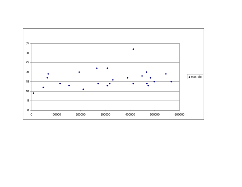
Figure 6: A scatter plot of the maximum edge distance between centers of two intersecting disks in a natural disk neighborhood system with the search expanded to include edges from a grid augmentation of the original road network.

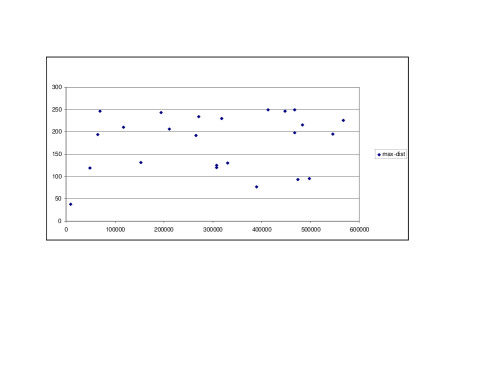
Figure 7: A scatter plot of the maximum edge distance between centers of two intersecting disks in a natural disk neighborhood system (distance searches where artificially cutoff after a depth of 250, so the distances could be even higher), without grid augmentations.

Let us assume, then, that we are given an $O(1)$-neighborly, bounded-degree, connected multiscale-dispersed graph, $G$, and we are interested in constructing an explicit representation of the intersection graph, $H$, for $G$’s natural disk neighborhood system. Furthermore, let us assume that we are given a list of all pairs of edges in $G$ that cross in the embedding of $G$ in ${\bf R}^{2}$, which converts $G$ into a plane graph, $G^{\prime}$. Moreover, since $G$ is a multiscale-dispersed graph, we have the following useful combinatorial lemma.

Suppose we are given the planarization $G^{\prime}$ of $G$. Thus, the plane graph $G^{\prime}$ has $O(n)$ vertices, which, in turn, implies that $G^{\prime}$ has $O(n)$ edges. Moreover, $G^{\prime}$ is connected, which implies that each face of $G^{\prime}$ can be viewed as a simple polygon, if we consider each edge as having a left side and a right side. Thus, we can compute a vertical trapezoidal decomposition of each face in $G^{\prime}$ in $O(n)$ time [9, 2] and we can similarly compute a horizontal trapezoidal decomposition of each face in $G^{\prime}$. By scanning these two trapezoidal decompositions, we can compute the grid augmentation, ${\hat{G}}$, of $G$. Since $G$ is $k$-neighborly, for some constant $k$, and $G$ has bounded degree, given any vertex $v$, we can find all the neighbors of $v$’s disk in $S$ by searching the $O(1)$ vertices in ${\hat{G}}$ that are at most $k$ edges away from $v$ in ${\hat{G}}$. Therefore, we have the following.

Lemma 7

Given an $n$-vertex $O(1)$-neighborly, bounded-degree, connected multiscale-dispersed graph, $G$, together with its planarization, $G$, we can construct an explicit representation of the intersection graph, $H$, of $G$’s natural disk neighborhood system, $S$, in $O(n)$ time.

5.2 Inductive $k$-Clustering

Suppose we are given a multiscale-dispersed graph, $G$, together with the disk intersection graph, $H$, for $G$’s natural disk neighborhood system, $S$. In particular, let us assume we have an explicit representation of $H$, such as in an adjacency list, with each vertex in $H$ labeled with its representative disk from $S$. For each vertex $v$ in $H$, let $R(v)$ denote the set of vertices in $H$ that are adjacent to $v$ and whose disk has radius no bigger that $v$’s disk. We say that $G$ is inductively $k$-clustered if, for each vertex $v$ in $H$, the number of connected components in $R(v)$ is no more than $k$. In the experimental section, we provide empirical evidence that real-world road networks are inductively $O(1)$-clustered (although the intersection graphs of their natural disk neighborhood systems do not necessarily have bounded degree). So, suppose that our given intersection graph, $H$, is for the natural disk neighborhood system, $S$, of an inductively $O(1)$-clustered multiscale-dispersed graph, $G$.

This characterization is justified by additional empirical evidence. Indeed, Figure 8 shows a scatter plot that supports the claim that real-world road networks are inductively $O(1)$-clustered, that is, the number of connected components of smaller disks neighboring a given disk is $O(1)$.

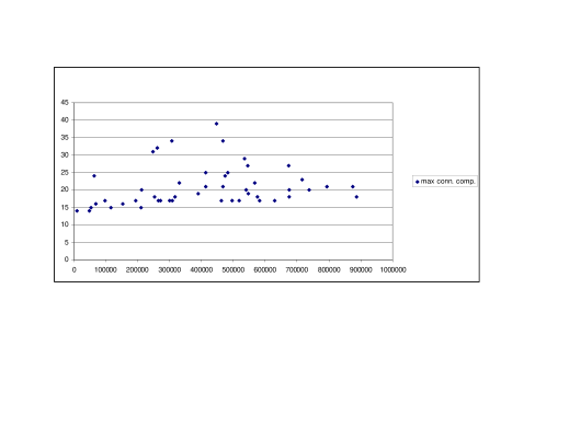
Figure 8: A scatter plot of the maximum number of connected components among smaller disks, which gives evidence that each road network is inductively $O(1)$-clustered.

By the way, an alternate approach for designing a linear-time algorithm for constructing an arrangement from an explicit representation of a disk network system is not supported by the data. Namely, it would be great if the vertex degrees in the disk neighborhood system were constant. Unfortunately, as shown in Figure 9, the distribution of maximum disk-intersection degrees does not appear to be constant. Indeed, it appears to be proportional to $\sqrt{n}$, which supports the “$O(\sqrt{n})$-exceptional” part of the notion of road networks as being subgraphs of $O(\sqrt{n})$-exceptional $O(1)$-ply disk systems.

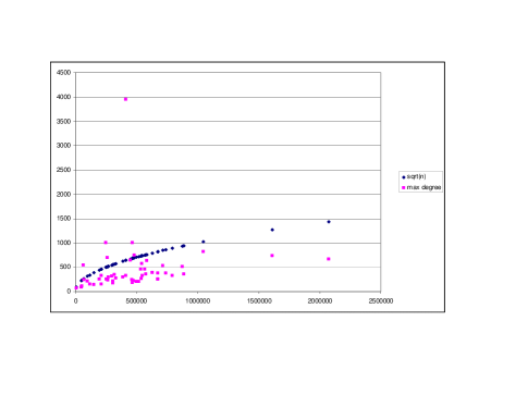
Figure 9: A scatter plot of the maximum vertex degrees for vertices in the natural disk neighborhood systems for TIGER/Line road networks, indexed by network size (the outlier is Louisiana), together with values for $\sqrt{n}$.

The inductive $k$-clustering property allows us to design a linear-time arrangement construction algorithm for $S$. Direct each edge in $H$ to go from $v$ to $w$ if the disk for $v$ is smaller than the disk for $w$, with ties broken using the indices of $v$ and $w$, so that the resulting graph $D$ is a directed acyclic graph. Note that, by Lemma 1, $H$ has $O(n)$ edges; hence, $D$ has $O(n)$ edges. Let us therefore perform a topological ordering of the vertices in $D$, which will take $O(n)$ time. Now, consider each vertex $v$ according to this topological ordering. In processing a vertex $v$ in this order, we may assume inductively that we have constructed the arrangement of all the circles associated with vertices in $R(v)$. Since there are $O(1)$ connected components in $R(v)$, each with its own subarrangement, we may sort these components radially, using the center of $v$’s circle as origin, in $O(1)$ time. Note that these connected components don’t intersect each other (by definition). So the arrangement of the circles in $R(v)$ and $v$’s circle can be constructed in $O(|R(v)|)$ time by “splicing” $v$’s circle into this arrangement using a traversal through each subarrangement (with the subarrangements considered in turn according to their radial order around $v$’s circle center). This gives us the following.

Lemma 8

Suppose we are given an $n$-vertex inductively $O(1)$-clustered multiscale-dispersed graph, $G$, together with the intersection graph, $H$, of $G$’s natural disk neighborhood system, $S$. Then we can construct the arrangement of the circles in $S$ in $O(n)$ time.

This lemma, together with Lemma 7, imply the following:

Theorem 9

Suppose we are given a bounded-degree $n$-vertex connected multiscale-dispersed graph, $G$, such that $G$ is $O(1)$-neighborly and inductively $O(1)$-clustered. Suppose further that we are given a planarization, $G^{\prime}$, of $G$. Then we can construct the arrangement of the circles in $G$’s natural disk neighborhood system, $S$, in $O(n)$ time.

6 Conclusions and Future Work

We have given a new theoretical characterization of road networks as multiscale-dispersed graphs and we have shown how this characterization leads to algorithms that provably run in linear time for a number of interesting problems. Our main techniques involve the construction of recursive $O(\sqrt{n})$-separator decompositions and the applications of such decompositions to Voronoi diagrams and shortest paths. In addition, we provided an algorithm for constructing the arrangement of the natural disk neighborhood system of a road network, utilization some additional properties of road networks, which are justified empirically.

There are a number of interesting open problems and future research directions raised by this paper, including:

• Can one construct a recursive circle $O(\sqrt{n})$-separator decomposition of a multiscale-dispersed graph deterministically in $O(n)$ time?

• Can one construct a trapezoidal decomposition of an $n$-vertex multiscale-dispersed graph in $O(n)$ time? (This is related to the well-known open problem of computing a trapezoidal decomposition of an $n$-vertex non-simple polygon in $O(n+k)$ time, where $k$ is the number of its edge crossings.)

• Are there a set of road network complexity measures, possibly based on our definitions, that can replace the Alpha and Gamma indices [12], which are used in the transportation network literature and are based on the flawed notion that road networks are plane graphs?

Of course, one can also perform additional experiments to empirically test whether real-world road networks possess additional properties not considered in this paper.

Acknowledgments

This work was supported in part by the NSF, under grant 0830403, and by the Office of Naval Research, under grant N00014-08-1-1015. With the exception of the images in Figure 3, all figures in this paper are the property of the authors and are used by permission.

References

- [1] L. Aceto and A. Ingolfsdottir. Computer Scientist: 21st Century Renaissance Man, 2007. http://www.ru.is/faculty/luca/PAPERS/renaissance-man.pdf.
- [2] N. M. Amato, M. T. Goodrich, and E. A. Ramos. A randomized algorithm for triangulating a simple polygon in linear time. Discrete Comput. Geom., 26(2):245–265, 2001.
- [3] D. Armon and J. Reif. A dynamic separator algorithm. In Proc. 3rd Workshop Algorithms Data Struct., volume 709 of Lecture Notes Comput. Sci., pages 107–118. Springer-Verlag, 1993.
- [4] S. Arora and B. Chazelle. Is the thrill gone? Commun. ACM, 48(8):31–33, 2005.
- [5] F. Aurenhammer. Voronoi diagrams: A survey of a fundamental geometric data structure. ACM Comput. Surv., 23(3):345–405, Sept. 1991.
- [6] F. Aurenhammer and R. Klein. Voronoi diagrams. In J.-R. Sack and J. Urrutia, editors, Handbook of Computational Geometry, pages 201–290. Elsevier Science Publishers B.V. North-Holland, Amsterdam, 2000.
- [7] M. Batty and P. Longley. Fractal Cities: A Geometry of Form and Function. Academic Press, 1994.
- [8] P. Bose and L. Devroye. On the stabbing number of a random Delaunay triangulation. Comput. Geom. Theory Appl., 36(2):89–105, 2007.
- [9] B. Chazelle. Triangulating a simple polygon in linear time. Discrete Comput. Geom., 6(5):485–524, 1991.
- [10] B. Chazelle. Could Your iPod Be Holding the Greatest Mystery in Modern Science? MAA Math Horizons (Codes, Cryptography, and National Security), 13, 2006. http://www.cs.princeton.edu/~chazelle/pubs/ipod.pdf.
- [11] B. Chazelle. The Algorithm: Idiom of Modern Science, 2006. http://www.cs.princeton.edu/~chazelle/pubs/algorithm.html.
- [12] Y. H. Chou. Exploring Spatial Analysis in GIS. Onword Press, 1996.
- [13] A. Condon. RNA Molecules: Glimpses Through an Algorithmic Lens. In LATIN 2006: Theoretical Informatics, volume 3887 of Springer LNCS, pages 8–10. Springer, 2006.
- [14] T. H. Cormen, C. E. Leiserson, R. L. Rivest, and C. Stein. Introduction to Algorithms. MIT Press, Cambridge, MA, 2nd edition, 2001.
- [15] G. Di Battista, P. Eades, R. Tamassia, and I. G. Tollis. Graph Drawing. Prentice Hall, Upper Saddle River, NJ, 1999.
- [16] D. Eppstein. Setting parameters by example. SIAM J. Computing, 32(3):643–653, 2003.
- [17] D. Eppstein, M. T. Goodrich, and D. Strash. Linear-time algorithms for geometric graphs with sublinearly many crossings. In SODA ’09: Proceedings of the Nineteenth Annual ACM -SIAM Symposium on Discrete Algorithms, pages 150–159, Philadelphia, PA, USA, 2009. Society for Industrial and Applied Mathematics.
- [18] D. Eppstein, G. L. Miller, and S.-H. Teng. A deterministic linear time algorithm for geometric separators and its applications. In Proc. 9th Annu. ACM Sympos. Comput. Geom., pages 99–108, 1993.
- [19] M. Erwig. The Graph Voronoi Diagram with Applications. Networks, 36(3):156–163, 2000.
- [20] J. W. Essam and M. E. Fisher. Some basic definitions in graph theory. Review of Modern Physics, 42(2):271–288, 1970.
- [21] M. L. Fredman and R. E. Tarjan. Fibonacci heaps and their uses in improved network optimization algorithms. J. ACM, 34:596–615, 1987.
- [22] A. V. Goldberg. Scaling algorithms for the shortest paths problem. In SODA ’93: Proceedings of the fourth annual ACM-SIAM Symposium on Discrete algorithms, pages 222–231, Philadelphia, PA, USA, 1993. Society for Industrial and Applied Mathematics.
- [23] A. V. Goldberg and C. Harrelson. Computing the shortest path: A∗ search meets graph theory. In SODA ’05: Proceedings of the sixteenth annual ACM-SIAM symposium on Discrete algorithms, pages 156–165, Philadelphia, PA, USA, 2005. Society for Industrial and Applied Mathematics.
- [24] M. T. Goodrich. Planar separators and parallel polygon triangulation. J. Comput. Syst. Sci., 51(3):374–389, 1995.
- [25] M. T. Goodrich and R. Tamassia. Algorithm Design: Foundations, Analysis, and Internet Examples. John Wiley & Sons, New York, NY, 2002.
- [26] M. R. Henzinger, P. Klein, S. Rao, and S. Subramanian. Faster shortest-path algorithms for planar graphs. J. Comput. Syst. Sci., 55(1):3–23, 1997.
- [27] M. Holzer, F. Schulz, D. Wagner, and T. Willhalm. Combining speed-up techniques for shortest-path computations. J. Exp. Algorithmics, 10:2.5, 2005.
- [28] G. A. Klunder and H. N. Post. The shortest path problem on large-scale real-road networks. Networks, 48(4):182–194, 2006.
- [29] P. Koebe. Kontaktprobleme der konformen Abbildung. Ber. Verh. Sächs. Akademie der Wissenschaften Leipzig, Math.-Phys. Klasse, 88:141–164, 1936.
- [30] R. J. Lipton and R. E. Tarjan. A separator theorem for planar graphs. SIAM J. Appl. Math., 36:177–189, 1979.
- [31] K. Mehlhorn. A Faster Approximation Algorithm for the Steiner Problem in Graphs. Information Processing Letters, 27:125–128, 1988.
- [32] U. Meyer. Single-source shortest-paths on arbitrary directed graphs in linear average-case time. In SODA ’01: Proceedings of the twelfth annual ACM-SIAM symposium on Discrete algorithms, pages 797–806, Philadelphia, PA, USA, 2001. Society for Industrial and Applied Mathematics.
- [33] G. L. Miller. Finding small simple cycle separators for 2-connected planar graphs. J. Comput. Syst. Sci., 32(3):265–279, 1986.
- [34] G. L. Miller, S.-H. Teng, W. Thurston, and S. A. Vavasis. Geometric separators for finite element meshes. SIAM J. Sci. Comput., 19(2):364–386, 1995.
- [35] G. L. Miller, S.-H. Teng, W. Thurston, and S. A. Vavasis. Separators for sphere-packings and nearest neighbor graphs. J. ACM, 44:1–29, 1997.
- [36] B. Mohar. A polynomial time circle packing algorithm. Discrete Math., 117:257–263, 1993.
- [37] J. Pach. Towards a Theory of Geometric Graphs, volume 342 of Contemporary Mathematics. American Mathematical Society, 2004.
- [38] C. Papadimitriou. The Algorithmic Lens: How the Computational Perspective is Transforming the Sciences, 2007. FCRC CCC presentation, http://lazowska.cs.washington.edu/fcrc/Christos.FCRC.pdf.
- [39] R. Raman. Recent results on the single-source shortest paths problem. SIGACT News, 28(2):81–87, 1997.
- [40] P. Sanders and D. Schultes. Highway Hierarchies Hasten Exact Shortest Path Queries. In Proceedings 17th European Symposium on Algorithms (ESA), volume 3669 of Springer LNCS, pages 568–579. Springer, 2005.
- [41] R. Sedgewick and J. S. Vitter. Shortest paths in Euclidean graphs. Algorithmica, 1:31–48, 1986.
- [42] D. A. Spielman and S.-H. Teng. Disk packings and planar separators. In Proc. 12th Annu. ACM Sympos. Comput. Geom., pages 349–358, 1996.
- [43] M. Thorup. Undirected single-source shortest paths with positive integer weights in linear time. J. ACM, 46(3):362–394, 1999.
- [44] W. T. Trotter. Planar Graphs, volume 9 of DIMACS Series in Discrete Mathematics and Theoretical Computer Science. American Mathematical Society, 1993.
- [45] J. M. Wing. Computational thinking. Commun. ACM, 49(3):33–35, 2006.
- [46] F. B. Zhan and C. E. Noon. Shortest Path Algorithms: An Evaluation Using Real Road Networks. Transportation Science, 32(1):65–73, 1998.