Flow Faster: Efficient Decision Algorithms for Probabilistic Simulations*

Abstract.

Strong and weak simulation relations have been proposed for Markov chains, while strong simulation and strong probabilistic simulation relations have been proposed for probabilistic automata. This paper investigates whether they can be used as effectively as their non-probabilistic counterparts. It presents drastically improved algorithms to decide whether some (discrete- or continuous-time) Markov chain strongly or weakly simulates another, or whether a probabilistic automaton strongly simulates another. The key innovation is the use of parametric maximum flow techniques to amortize computations. We also present a novel algorithm for deciding strong probabilistic simulation preorders on probabilistic automata, which has polynomial complexity via a reduction to an LP problem. When extending the algorithms for probabilistic automata to their continuous-time counterpart, we retain the same complexity for both strong and strong probabilistic simulations.

1. Introduction

Many verification methods have been introduced to prove the correctness of systems exploiting rigorous mathematical foundations. As one of the automatic verification techniques, model checking has successfully been applied to automatically find errors in complex systems. The power of model checking is limited by the state space explosion problem. Notably, minimizing the system to the bisimulation [34, 35] quotient is a favorable approach. As a more aggressive attack to the problem, simulation relations [33] have been proposed for these models. In particular, they provide the principal ingredients to perform abstractions of the models, while preserving safe CTL properties (formulas with positive universal path-quantifiers only) [16].

Simulation relations are preorders on the state space such that whenever state $s^{\prime}$ simulates state $s$ (written $s\precsim s^{\prime}$) then $s^{\prime}$ can mimic all stepwise behaviour of $s$, but $s^{\prime}$ may perform steps that cannot be matched by $s$. One of the interesting aspects of simulation relations is that they allow a verification by “local” reasoning. Based on this, efficient algorithms for deciding simulation preorders have been proposed in [10, 23].

Randomisation has been employed widely for performance and dependability models, and consequently the study of verification techniques of probabilistic systems with and without nondeterminism has drawn a lot of attention in recent years. A variety of equivalence and preorder relations, including strong and weak simulation relations, have been introduced and widely considered for probabilistic models. In this paper we consider discrete-time Markov chains (DTMCs) and discrete-time probabilistic automata (PAs) [39]. PAs extend labelled transition systems (LTSs) with probabilistic selection, or, viewed differently, extend DTMCs with nondeterminism. They constitute a natural model of concurrent computation involving random phenomena. In a PA, a labelled transition leads to a probability distribution over the set of states, rather than a single state. The resulting model thus exhibits both non-deterministic choice (as in LTSs) and probabilistic choice (as in Markov chains).

Strong simulation relations have been introduced [26, 30] for probabilistic systems. For $s\precsim s^{\prime}$ ($s^{\prime}$ strongly simulates $s$), it is required that every successor distribution of $s$ via action $\alpha$ (called $\alpha$-successor distribution) has a corresponding $\alpha$-successor distribution at $s^{\prime}$. Correspondence of distributions is naturally defined with the concept of weight functions [26]. In the context of model checking, strong simulation relations preserve safe PCTL formulas [40]. Probabilistic simulation [40] is a relaxation of strong simulation in the sense that it allows for convex combinations of multiple distributions belonging to equally labelled transitions. More concretely, it may happen that for an $\alpha$-successor distribution $\mu$ of $s$, there is no $\alpha$-successor distribution of $s^{\prime}$ which can be related to $\mu$, yet there exists a so-called $\alpha$-combined transition, a convex combination of several $\alpha$-successor distributions of $s^{\prime}$. Probabilistic simulation accounts for this and is thus coarser than strong simulation, but still preserves the same class of PCTL-properties as strong simulation does.

Apart from discrete time models, this paper considers continuous-time Markov chains (CTMCs) and continuous-time probabilistic automata (CPAs) [29, 42]. In CPAs, the transition delays are governed by exponential distributions. CPAs can be considered also as extensions of CTMCs with nondeterminism. CPAs are natural foundational models for various performance and dependability modelling formalisms including stochastic activity networks [37], generalised stochastic Petri nets [32] and interactive Markov chains [24]. Strong simulation and probabilistic simulation have been introduced for continuous-time models [9, 44]. For CTMCs, $s\precsim s^{\prime}$ requires that $s\precsim s^{\prime}$ holds in the embedded DTMC, and additionally, state $s^{\prime}$ must be “faster” than $s$ which manifests itself by a higher exit rate. Both strong simulation and probabilistic simulation preserve safe CSL formulas [4], which is a continuous stochastic extension of PCTL, tailored to continuous-time models.

Weak simulation is proposed in [9] for Markov chains. In weak simulation, the successor states are split into visible and invisible parts, and the weight function conditions are only imposed on the transitions leading to the visible parts of the successor states. Weak simulation is strictly coarser than the afore-mentioned strong simulation for Markov chains, thus allows further reduction of the state space. It preserves the safe PCTL- and CSL-properties without the next state formulas for DTMCs and CTMCs respectively [9].

Decision algorithms for strong and weak simulations over Markov chains, and for strong simulation over probabilistic automata are not efficient, which makes it as yet unclear whether they can be used as effectively as their non-probabilistic counterparts. In this paper we improve efficient decision algorithms, and devise new algorithms for deciding strong and strong probabilistic simulations for probabilistic automata. Given the simulation preorder, the simulation quotient automaton is in general smaller than the bisimulation quotient automaton. Then, for safety and liveness properties, model checking can be performed on this smaller quotient automata. The study of decision algorithms is also important for specification relations: The model satisfies the specification if the automaton for the specification simulates the automaton for the model. In many applications the specification cannot be easily expressed by logical formulas: it is rather a probabilistic model itself. Examples of this kind include various recent wireless network protocols, such as ZigBee [21], Firewire Zeroconf [11], or the novel IEEE 802.11e, where the central mechanism is selecting among different-sided dies, readily expressible as a probabilistic automaton [31].

The common strategy used by decision algorithms for simulations is as follows. The algorithm starts with a relation $R$ which is guaranteed to be coarser than the simulation preorder $\precsim$. Then, the relation $R$ is successively be refined. In each iteration of the refinement loop, pairs $(s,s^{\prime})$ are eliminated from the relation $R$ if the corresponding simulation conditions are violated with respect to the current relation. In the context of labelled transitions systems, this happens if $s$ has a successor state $t$, but we cannot find a successor state $t^{\prime}$ of $s^{\prime}$ such that $(t,t^{\prime})$ is also in the current relation $R$. For DTMCs, this correspondence is formulated by the existence of a weight function for distributions $(\mathbf{P}(s,\cdot),\mathbf{P}(s^{\prime},\cdot))$ with respect to the current relation $R$. Checking this weight function condition amounts to checking whether there is a maximum flow over the network constructed out of $(\mathbf{P}(s,\cdot),\mathbf{P}(s^{\prime},\cdot))$ and the current relation $R$. The complexity for one such check is however rather expensive, it has time complexity $\mathcal{O}(n^{3}/\log n)$. If the iterative algorithm reaches a fix-point, the strong simulation preorder is obtained. The number of iterations of the refinement loop is at most $\mathcal{O}(n^{2})$, and the overall complexity [3] amounts to $\mathcal{O}(n^{7}/\log n)$ in time and $\mathcal{O}(n^{2})$ in space.

Fixing a pair $(s,s^{\prime})$, we observe that the networks for this pair across iterations of the refinement loop are very similar: They differ from iteration to iteration only by deletion of some edges induced by the successive clean up of $R$. We exploit this by adapting a parametric maximum flow algorithm [18] to solve the maximum flow problems for the arising sequences of similar networks, hence arriving at efficient simulation decision algorithms. The basic idea is that all computations concerning the pair $(s,s^{\prime})$ can be performed in an incremental way: after each iteration we save the current network together with maximum flow information. Then, in the next iteration, we update the network, and derive the maximum flow while using the previous maximum flow function. The maximum flow problems for the arising sequences of similar networks with respect to the pair $(s,s^{\prime})$ can be computed in time $\mathcal{O}(|V|^{3})$ where $|V|$ is the number of nodes of the network. This leads to an overall time complexity $\mathcal{O}(m^{2}n)$ for deciding the simulation preorder. Because of the storage of the networks, the space complexity is increased to $\mathcal{O}(m^{2})$. Especially in the very common case where the state fanout of a model is bounded by a constant $g$ (and hence $m\leq gn$), our strong simulation algorithm has time and space complexity $\mathcal{O}(n^{2})$. The algorithm can be extended easily to handle CTMCs with same time and space complexity. For weak simulation on Markov chains, the parametric maximum flow technique cannot be applied directly. Nevertheless, we manage to incorporate the parametric maximum flow idea into a decision algorithm with time complexity $\mathcal{O}(m^{2}n^{3})$ and space complexity $\mathcal{O}(n^{2})$. An earlier algorithm [6] uses LP problems [27, 38] as subroutines. The maximum flow problem is a special instance of an LP problem but can be solved much more efficiently [1].

We extend the algorithm to compute strong simulation preorder to also work on PAs. It takes the skeleton of the algorithm for Markov chains: It starts with a relation $R$ which is coarser than $\precsim$, and then refines $R$ until $\precsim$ is achieved. In the refinement loop, a pair $(s,s^{\prime})$ is eliminated if the corresponding simulation conditions are violated with respect to the current relation. For PAs, this means that there exists an $\alpha$-successor distribution $\mu$ of $s$, such that for all $\alpha$-successor distribution $\mu^{\prime}$ of $s^{\prime}$, we cannot find a weight function for $(\mu,\mu^{\prime})$ with respect to the current relation $R$. Again, as for Markov chains, the existence of such weight functions can be reduced to maximum flow problems. Combining with the parametric maximum flow algorithm [18], we arrive at the same time complexity $\mathcal{O}(m^{2}n)$ and space complexity $\mathcal{O}(m^{2})$ as for Markov chains. The above maximum flow based procedure cannot be applied to deal with strong probabilistic simulation for PAs. The reason is that an $\alpha$-combined transition of state $s$ is a convex combination of several $\alpha$-successor distributions of $s$, thus induces uncountable many such possible combined transitions. The computational complexity of deciding strong probabilistic simulation has not been investigated before. We show that it can be reduced to solving LP problems. The idea is that we introduce for each $\alpha$-successor distribution a variable, and then reformulates the requirements concerning the combined transitions by linear constraints over these variables. This allows us to construct a set of LP problem such that whether a pair $(s,s^{\prime})$ should be thrown out of the current pair $R$ is equivalent to whether each of the LP problem has a solution.

The algorithms for PAs are then extended to handle their continuous-time analogon, CPAs. In the algorithm, for each pair $(s,s^{\prime})$ in the refinement loop, an additional rate condition is ensured by an additional check via comparing the appropriate rates of $s$ and $s^{\prime}$. The resulting algorithm has the same time and space complexity.

Related Works

In the non-probabilistic setting, the most efficient algorithms for deciding simulation preorders have been proposed in [10, 23]. The complexity is $\mathcal{O}(mn)$ where $n$ and $m$ denote the number of states and transitions of the transition system respectively. For Markov chains, Derisavi et al. [17] presented an $\mathcal{O}(m\log n)$ algorithm for strong bisimulation. Weak bisimulation for DTMCs can be computed in $\mathcal{O}(n^{3})$ time [5]. For strong simulation, Baier et al. [3] introduced a polynomial decision algorithm with complexity $\mathcal{O}(n^{7}/\log n)$, by tailoring a network flow algorithm [20] to the problem, embedded into an iterative refinement loop. In [6], Baier et al. proved that weak simulation is decidable in polynomial time by reducing it to linear programming (LP) problems. For a subclass of PAs (reactive systems), Huynh and Tian [25] presented an $\mathcal{O}(m\log n)$ algorithm for computing strong bisimulation. Cattani and Segala [12] have presented decision algorithms for strong and bisimulation for PAs. They reduced the decision problems to LP problems. To compute the coarsest strong simulation for PAs, Baier et al.  [3] presented an algorithm which reduces the query whether a state strongly simulates another to a maximum flow problem. Their algorithm has complexity $\mathcal{O}((mn^{6}+m^{2}n^{3})/\log n)$. Recently, algorithm for computing simulation and bisimulation metrics for concurrent games [13] has been studied.

Outline of The Paper

The paper proceeds by recalling the definition of the models and simulation relations in Section 2. In Section 3 we give a short interlude on maximum flow problems. In Section 4 we present a combinatorial method to decide strong simulations. In this section we also introduce new decision algorithms for deciding strong probabilistic simulations for PAs and CPAs. In Section 5 we focus on algorithms for weak simulations. Section 6 concludes the paper.

2. Preliminaries

In Subsection 2.1, we recall the definitions of fully probabilistic systems, discrete- and continuous-time Markov chains [41], and the nondeterministic extensions of these discrete-time [40] and continuous-time models [36, 7]. In Subsection 2.2 we recall the definition of simulation relations.

2.1. Markov Models

Firstly, we introduce some general notations. Let $X,Y$ be finite sets. For $f:X\to\mathbb{R}$, let $f(A)$ denote $\sum_{x\in A}f(x)$ for all $A\subseteq X$. For $f:X\times Y\to\mathbb{R}$, we let $f(x,A)$ denote $\sum_{y\in A}f(x,y)$ for all $x\in X$ and $A\subseteq Y$, and $f(A,y)$ is defined similarly. Let $AP$ be a fixed, finite set of atomic propositions.

For a finite set $S$, a distribution $\mu$ over $S$ is a function $\mu:S\to[0,1]$ satisfying the condition $\mu(S)\leq 1$. The support of $\mu$ is defined by $\mathit{Supp}(\mu)=\{s\mid\mu(s)>0\}$, and the size of $\mu$ is defined by $\left\lvert\mu\right\rvert=\left\lvert\mathit{Supp}(\mu)\right\rvert$. The distribution $\mu$ is called stochastic if $\mu(S)=1$, absorbing if $\mu(S)=0$. We sometimes use an auxiliary state (not a real state) ${\mathord{\bot}}\not\in S$ and set $\mu({\mathord{\bot}})=1-\mu(S)$. If $\mu$ is not stochastic we have $\mu({\mathord{\bot}})>0$. Further, let $S_{\mathord{\bot}}$ denote the set $S\cup\{{\mathord{\bot}}\}$, and let $\mathit{Supp}_{\mathord{\bot}}(\mu)=\mathit{Supp}(\mu)\cup\{{\mathord{\bot}}\}$ if $\mu({\mathord{\bot}})>0$ and $\mathit{Supp}_{\mathord{\bot}}(\mu)=\mathit{Supp}(\mu)$ otherwise. We let $\mathit{Dist}(S)$ denote the set of distributions over the set $S$.

A labelled fully probabilistic system (FPS) is a tuple $\mathcal{M}=(S,\mathbf{P},L)$ where $S$ is a finite set of states, $\mathbf{P}:S\times S\to[0,1]$ is a probability matrix such that $\mathbf{P}(s,\cdot)\in\mathit{Dist}(S)$ for all $s\in S$, and $L:S\to 2^{AP}$ is a labelling function.

A state $s$ is called stochastic and absorbing if the distribution $\mathbf{P}(s,\cdot)$ is stochastic and absorbing respectively. For $s\in S$, let $\mathit{post}(s)=\mathit{Supp}(\mathbf{P}(s,\cdot))$, and let $\mathit{post}_{\mathord{\bot}}(s)=\mathit{Supp}_{\mathord{\bot}}(\mathbf{P}(s,\cdot))$.

A labelled discrete-time Markov chain (DTMC) is an FPS $\mathcal{M}=(S,\mathbf{P},L)$ where $s$ is either absorbing or stochastic for all $s\in S$.

FPSs and DTMCs are time-abstract, since the duration between triggering transitions is disregarded. We observe the state only at a discrete set of time points $0,1,2,\ldots$. We recall the definition of CTMCs which are time-aware:

A labelled continuous-time Markov chain (CTMC) is a tuple $\mathcal{M}=(S,\mathbf{R},L)$ with $S$ and $L$ as before, and $\mathbf{R}:S\times S\to\mathbb{R}_{\geq 0}$ is a rate matrix.

For CTMC $\mathcal{M}$, let $\mathit{post}(s)=\{s^{\prime}\in S\mid\mathbf{R}(s,s^{\prime})>0\}$ for all $s\in S$. The rates give the average delay of the corresponding transitions. Starting from state $s$, the probability that within time $t$ a successor state is chosen is given by $1-e^{-\mathbf{R}(s,S)t}$. The probability that a specific successor state $s^{\prime}$ is chosen within time $t$ is thus given by $(1-e^{-\mathbf{R}(s,S)t})\cdot\mathbf{R}(s,s^{\prime})/\mathbf{R}(s,S)$. A CTMC induces an embedded DTMC, which captures the time-abstract behaviour of it:

Let $\mathcal{M}=(S,\mathbf{R},L)$ be a CTMC. The embedded DTMC of $\mathcal{M}$ is defined by $emb(\mathcal{M})=(S,\mathbf{P},L)$ with $\mathbf{P}(s,s^{\prime})=\mathbf{R}(s,s^{\prime})/\mathbf{R}(s,S)$ if $\mathbf{R}(s,S)>0$ and $0$ otherwise. We will also use $\mathbf{P}$ for a CTMC directly, without referring to its embedded DTMC explicitly. If one is interested in time-abstract properties (e. g., the probability to reach a set of states) of a CTMC, it is sufficient to analyse its embedded DTMC.

For a given FPS, DTMC or CTMC, its fanout is defined by $\max_{s\in S}\left\lvert\mathit{post}(s)\right\rvert$. The number of states is defined by $n=\left\lvert S\right\rvert$, and the number of transitions is defined by $m=\sum_{s\in S}\left\lvert\mathit{post}(s)\right\rvert$. For $s\in S$, $reach(s)$ denotes the set of states that are reachable from $s$ with positive probability. For a relation $R\subseteq S\times S$ and $s\in S$, let $R(s)$ denote the set $\{s^{\prime}\in S\mid(s,s^{\prime})\in R\}$. Similarly, for $s^{\prime}\in S$, let $R^{-1}(s^{\prime})$ denote the set $\{s\in S\mid(s,s^{\prime})\in R\}$. If $(s,s^{\prime})\in R$, we write also $s\mathrel{R}s^{\prime}$.

Markov chains are purely probabilistic. Now we consider extensions of Markov chains with nondeterminism. We first recall the definition of probabilistic automata, which can be considered as the simple probabilistic automata with transitions allowing deadlocks in [39].

A probabilistic automaton (PA) is a tuple $\mathcal{M}=(S,Act,\mathbf{P},L)$ where $S$ and $L$ are defined as before, $Act$ is a finite set of actions, $\mathbf{P}\subseteq S\times Act\times\mathit{Dist}(S)$ is a finite set, called the probabilistic transition matrix.

For $(s,\alpha,\mu)\in\mathbf{P}$, we use $s\xrightarrow{\alpha}\mu$ as a shorthand notation, and call $\mu$ an $\alpha$-successor distribution of $s$. Let $Act(s)=\{\alpha\mid\exists\mu:s\xrightarrow{\alpha}\mu\}$ denote the set of actions enabled at $s$. For $s\in S$ and $\alpha\in Act(s)$, let $Steps_{\alpha}(s)=\{\mu\in\mathit{Dist}(S)\mid s\xrightarrow{\alpha}\mu\}$ and $\mathit{Steps}(s)=\bigcup_{\alpha\in Act(s)}Steps_{\alpha}(s)$. The fanout of a state $s$ is defined by $\mathit{fan}(s)=\sum_{\alpha\in Act(s)}\sum_{\mu\in Steps_{\alpha}(s)}(\left\lvert\mu\right\rvert+1)$. Intuitively, $\mathit{fan}(s)$ denotes the total sum of the sizes of outgoing distributions of state $s$ plus their labelling. The fanout of $\mathcal{M}$ is defined by $\max_{s\in S}\mathit{fan}(s)$. Summing up over all states, we define the size of the transitions by $m=\sum_{s\in S}\mathit{fan}(s)$.

A Markov decision process (MDP) [36] arises from a PA $\mathcal{M}$ if for $s\in S$ and $\alpha\in Act$, there is at most one $\alpha$-successor distribution $\mu$ of $s$, which must be stochastic.

We consider a continuous-time counterpart of PAs where the transitions are described by rates instead of probabilities. A rate function is simply a function $r:S\to\mathbb{R}_{\geq 0}$. Let $\left\lvert r\right\rvert=\left\lvert\{s\mid r(s)>0\}\right\rvert$ denote the size of $r$. Let $\mathit{Rate}(S)$ denote the set of all rate functions. A continuous-time PA (CPA) is a tuple $(S,Act,\mathbf{R},L)$ where $S$, $Act$, $L$ as defined for PAs, and $\mathbf{R}\subseteq S\times Act\times\mathit{Rate}(S)$ a finite set, called the rate matrix. We write $s\xrightarrow{\alpha}r$ if $(s,\alpha,r)\in\mathbf{R}$, and call $r$ an $\alpha$-successor rate function of $s$. For transition $s\xrightarrow{\alpha}r$, the sum $r(S)$ is also called the exit rate of it. Given that the transition $s\xrightarrow{\alpha}r$ is chosen from state $s$, the probability that any successor state is chosen within time $t$ is given by $1-e^{-r(S)t}$, and a specific successor state $s^{\prime}$ is chosen within time $t$ is given by $(1-e^{-r(S)t})\cdot\frac{r(s^{\prime})}{r(S)}$. The notion of $Act(s)$, $Steps_{\alpha}(s)$, $\mathit{Steps}(s)$, fanout and size of transitions for PAs can be extended to CPAs by replacing occurrence of distribution $\mu$ by rate function $r$ in an obvious way.

The model continuous-time Markov decision processes (CTMDPs) [36, 7] can be considered as special CPAs where for $s\in S$ and $\alpha\in Act$, there exists at most one rate function $r\in\mathit{Rate}(S)$ such that $s\xrightarrow{\alpha}r$. The model CTMDPs considered in paper [42] essentially agree with our CPAs.

2.2. Strong and Weak Simulation Relations

We first recall the notion of strong simulation on Markov chains [9], PAs [40], and CPAs [44]. Strong probabilistic simulation is defined in Subsection 2.2.2. Weak simulation for Markov chains will be given in Subsection 2.2.3. The notion of simulation up to $R$ is introduced in Subsection 2.2.4.

2.2.1. Strong Simulation

Strong simulation requires that each successor distribution of one state has a corresponding successor distribution of the other state. The correspondence of distributions is naturally defined with the concept of weight functions [26], adapted to FPSs as in [9]. For a relation $R\subseteq S\times S$, we let $R_{\mathord{\bot}}$ denote the set $R\cup\{({\mathord{\bot}},s)\mid s\in S_{\mathord{\bot}}\}$.

Let $\mu,\mu^{\prime}\in\mathit{Dist}(S)$ and $R\subseteq S\times S$. A weight function for $(\mu,\mu^{\prime})$ with respect to $R$ is a function $\Delta:S_{\mathord{\bot}}\times S_{\mathord{\bot}}\rightarrow[0,1]$ such that

1. $\Delta(s,s^{\prime})>0$ implies $s\mathrel{R_{\mathord{\bot}}}s^{\prime}$,

2. $\mu(s)=\Delta(s,S_{\mathord{\bot}})$ for $s\in S_{\mathord{\bot}}$ and

3. $\mu^{\prime}(s^{\prime})=\Delta(S_{\mathord{\bot}},s^{\prime})$ for $s^{\prime}\in S_{\mathord{\bot}}$.

We write $\mu\sqsubseteq_{R}\mu^{\prime}$ if there exists a weight function for $(\mu,\mu^{\prime})$ with respect to $R$.

The first condition requires that only pairs $(s,s^{\prime})$ in the relation $R_{\mathord{\bot}}$ have a positive weight. In other words, for $s,s^{\prime}\in S$ with $s^{\prime}\not\in R_{\mathord{\bot}}(s)$, it holds that $\Delta(s,s^{\prime})=0$. Strong simulation requires similar states to be related via weight functions on their distributions [26].

Let $\mathcal{M}=(S,\mathbf{P},L)$ be an FPS, and let $R\subseteq S\times S$. The relation $R$ is a strong simulation on $\mathcal{M}$ iff for all $s_{1},s_{2}$ with $s_{1}\mathrel{R}s_{2}$: $L(s_{1})=L(s_{2})$ and $\mathbf{P}(s_{1},\cdot)\sqsubseteq_{R}\mathbf{P}(s_{2},\cdot)$.

We say that $s_{2}$ strongly simulates $s_{1}$ in $\mathcal{M}$, denoted by $s_{1}\precsim_{\mathcal{M}}s_{2}$, iff there exists a strong simulation $R$ on $\mathcal{M}$ such that $s_{1}\mathrel{R}s_{2}$.

By definition, it can be shown [9] that $\precsim_{\mathcal{M}}$ is reflexive and transitive, thus a preorder. Moreover, $\precsim_{\mathcal{M}}$ is the coarsest strong simulation relation for $\mathcal{M}$. If the model $\mathcal{M}$ is clear from the context, the subscript $\mathcal{M}$ may be omitted. Assume that $s_{1}\precsim s_{2}$ and let $\Delta$ denote the corresponding weight function. If $\mathbf{P}(s_{2},\bot)>0$, we have that $\mathbf{P}(s_{2},\bot)=\sum_{s\in S_{\bot}}\Delta(s,\bot)=\Delta({\mathord{\bot}},{\mathord{\bot}})$. The second equality follows by the fact that $\bot$ can not strongly simulate any real state in $S$. Another observation is that if $s$ is absorbing, then it can be strongly simulated by any other state $s^{\prime}$ with $L(s)=L(s^{\prime})$.

$s_{1}$[fillstyle=solid,fillcolor=yellow]$u_{1}$ $\frac{1}{2}$ $v_{1}$ $\frac{1}{4}$ [fillstyle=solid,fillcolor=yellow]$q_{1}$ $\frac{1}{8}$           $s_{2}$[fillstyle=solid,fillcolor=yellow]$u_{2}$ $\frac{1}{2}$ $v_{2}$ $\frac{1}{2}$ [fillstyle=solid,fillcolor=yellow]$q_{2}$ $\frac{1}{8}$ [fillstyle=solid,fillcolor=BlueGreen]$q_{3}$ $\frac{3}{4}$           $s_{3}$[fillstyle=solid,fillcolor=yellow]$u_{3}$ $\frac{2}{3}$ $v_{3}$ $\frac{1}{3}$ [fillstyle=solid,fillcolor=yellow]$q_{4}$ $\frac{1}{8}$ [fillstyle=solid,fillcolor=BlueGreen]$q_{5}$ $\frac{7}{8}$

Figure 1. An FPS for illustrating the simulation relations.

Consider the FPS depicted in Figure 3. Recall that labelling of states is indicated by colours in the states. Since the yellow (grey) states are absorbing, they strongly simulate each other. The same holds for the green (dark grey) states. We show now that $s_{1}\precsim s_{2}$ but $s_{2}\not\precsim s_{3}$.

Consider first the pair $(s_{1},s_{2})$. Let $R=\{(s_{1},s_{2}),(u_{1},u_{2}),(v_{1},v_{2}),(q_{1},q_{2})\}$. We show that $R$ is a strong simulation relation. First observe that $L(s)=L(s^{\prime})$ for all $(s,s^{\prime})\in R$. Since states $u_{1},q_{1}$ are absorbing, the conditions for the pairs $(u_{1},u_{2})$ and $(q_{1},q_{2})$ hold trivially. To show the conditions for $(v_{1},v_{2})$, we consider the function $\Delta_{1}$ defined by: $\Delta_{1}(q_{1},q_{2})=\frac{1}{8}$, $\Delta_{1}({\mathord{\bot}},q_{3})=\frac{3}{4}$, $\Delta_{1}({\mathord{\bot}},{\mathord{\bot}})=\frac{1}{8}$ and $\Delta_{1}(\cdot)=0$ otherwise. It is easy to check that $\Delta_{1}$ is a weight function for $(\mathbf{P}(v_{1},\cdot),\mathbf{P}(v_{2},\cdot))$ with respect to $R$. Now consider $(s_{1},s_{2})$. The weight function $\Delta_{2}$ for $(\mathbf{P}(s_{1},\cdot),\mathbf{P}(s_{2},\cdot))$ with respect to $R$ is given by $\Delta_{2}(u_{1},u_{2})=\frac{1}{2}$ and $\Delta_{2}(v_{1},v_{2})=\Delta_{2}({\mathord{\bot}},v_{2})=\frac{1}{4}$ and $\Delta_{2}(\cdot)=0$ otherwise. Thus $R$ is a strong simulation which implies that $s_{1}\precsim s_{2}$.

Consider the pair $(s_{2},s_{3})$. Since $\mathbf{P}(s_{2},v_{2})=\frac{1}{2}$, to establish the Condition 2 of Definition 2.2.1, we should have $\frac{1}{2}=\Delta(v_{2},S_{\mathord{\bot}})$. Observe that $v_{3}$ is the only successor state of $s_{3}$ which can strongly simulate $v_{2}$, thus $\Delta(v_{2},S_{\mathord{\bot}})=\Delta(v_{2},v_{3})$. However, for state $v_{3}$ we have $\mathbf{P}(s_{3},v_{3})<\Delta(v_{2},v_{3})$, which violates the Condition 3 of Definition 2.2.1, thus we cannot find such a weight function. Hence, $s_{2}\not\precsim s_{3}$.

Since each DTMC is a special case of an FPS, Definition 2.2.1 applies directly for DTMCs. For CTMCs we say that $s_{2}$ strongly simulates $s_{1}$ if, in addition to the DTMC conditions, $s_{2}$ can move stochastically faster than $s_{1}$ [9], which manifests itself by a higher rate.

Let $\mathcal{M}=(S,\mathbf{R},L)$ be a CTMC and let $R\subseteq S\times S$. The relation $R$ is a strong simulation on $\mathcal{M}$ iff for all $s_{1},s_{2}$ with $s_{1}\mathrel{R}s_{2}$: $L(s_{1})=L(s_{2})$, $\mathbf{P}(s_{1},\cdot)\sqsubseteq_{R}\mathbf{P}(s_{2},\cdot)$ and $\mathbf{R}(s_{1},S)\leq\mathbf{R}(s_{2},S)$.

We say that $s_{2}$ strongly simulates $s_{1}$ in $\mathcal{M}$, denoted by $s_{1}\precsim_{\mathcal{M}}s_{2}$, iff there exists a strong simulation $R$ on $\mathcal{M}$ such that $s_{1}\mathrel{R}s_{2}$.

Thus, $s\precsim_{\mathcal{M}}s^{\prime}$ holds if $s\precsim_{emb(\mathcal{M})}s^{\prime}$, and $s^{\prime}$ is faster than $s$. By definition, it can be shown that $\precsim_{\mathcal{M}}$ is a preorder, and is the coarsest strong simulation relation for $\mathcal{M}$. For PAs, strong simulation requires that every $\alpha$-successor distribution of $s_{1}$ is related to an $\alpha$-successor distribution of $s_{2}$ via a weight function [40, 26]: Let $\mathcal{M}=(S,Act,\mathbf{P},L)$ be a PA and let $R\subseteq S\times S$. The relation $R$ is a strong simulation on $\mathcal{M}$ iff for all $s_{1},s_{2}$ with $s_{1}\mathrel{R}s_{2}$: $L(s_{1})=L(s_{2})$ and if $s_{1}\xrightarrow{\alpha}\mu_{1}$ then there exists a transition $s_{2}\xrightarrow{\alpha}\mu_{2}$ with $\mu_{1}\sqsubseteq_{R}\mu_{2}$.

We say that $s_{2}$ strongly simulates $s_{1}$ in $\mathcal{M}$, denoted $s_{1}\precsim_{\mathcal{M}}s_{2}$, iff there exists a strong simulation $R$ on $\mathcal{M}$ such that $s_{1}\mathrel{R}s_{2}$.

Figure 2. A PA for illustrating the simulation relations.

Consider the PA in Figure 2. Then, it is easy to check $s_{1}\precsim s_{2}$: each $\alpha$-successor distribution of $s_{1}$ has a corresponding $\alpha$-successor distribution of $s_{2}$. However, $s_{1}$ does not strongly simulate $s_{2}$, as the middle $\alpha$-successor distribution of $s_{2}$ can not be related by any $\alpha$-successor distribution of $s_{1}$.

Now we consider CPAs. For a rate function $r$, we let $\mu(r)\in\mathit{Dist}(S)$ denote the induced distribution defined by: if $r(S)>0$ then $\mu(r)(s)$ equals $r(s)/r(S)$ for all $s\in S$, and if $r(S)=0$, then $\mu(r)(s)=0$ for all $s\in S$. Now we introduce the notion of strong simulation for CPAs [44], which can be considered as an extension of the definition for CTMCs [9]:

Let $\mathcal{M}=(S,Act,\mathbf{R},L)$ be a CPA and let $R\subseteq S\times S$. The relation $R$ is a strong simulation on $\mathcal{M}$ iff for all $s_{1},s_{2}$ with $s_{1}\mathrel{R}s_{2}$: $L(s_{1})=L(s_{2})$ and if $s_{1}\xrightarrow{\alpha}r_{1}$ then there exists a transition $s_{2}\xrightarrow{\alpha}r_{2}$ with $\mu(r_{1})\sqsubseteq_{R}\mu(r_{2})$ and $r_{1}(S)\leq r_{2}(S)$.

We write $s_{1}\precsim_{\mathcal{M}}s_{2}$ iff there exists a strong simulation $R$ on $\mathcal{M}$ such that $s_{1}\mathrel{R}s_{2}$.

Similar to CTMCs, the additional rate condition $r_{1}(S)\leq r_{2}(S)$ indicates that the transition $s_{2}\xrightarrow{\alpha}r_{2}$ is faster than $s_{1}\xrightarrow{\alpha}r_{1}$. As a shorthand notation, we use $r_{1}\sqsubseteq_{R}r_{2}$ for the condition $\mu(r_{1})\sqsubseteq_{R}\mu(r_{2})$ and $r_{1}(S)\leq r_{2}(S)$. For both PAs and CPAs, $\precsim_{\mathcal{M}}$ is the coarsest strong simulation relation.

2.2.2. Strong Probabilistic Simulations

We recall the definition of strong probabilistic simulation, which is coarser than strong simulation, but still preserves the same class of PCTL-properties as strong simulation does. We first recall the notion of combined transition [39], a convex combination of several equally labelled transitions:

Let $\mathcal{M}=(S,Act,\mathbf{P},L)$ be a PA. Let $s\in S$, $\alpha\in Act(s)$ and $k=\left\lvert\mathit{Steps}_{\alpha}(s)\right\rvert$. Assume that $\mathit{Steps}_{\alpha}(s)=\{\mu_{1},\ldots,\mu_{k}\}$. The tuple $(s,\alpha,\mu)$ is a combined transition, denoted by $s\stackrel{{\scriptstyle\alpha}}{{\leadsto}}\mu$, iff there exist constants $c_{1},\ldots,c_{k}\in[0,1]$ with $\sum_{i=1}^{k}c_{i}=1$ such that $\mu=\sum_{i=1}^{k}c_{i}\mu_{i}$.

The key difference to Definition 1 is the use of $\stackrel{{\scriptstyle\alpha}}{{\leadsto}}$ instead of $\xrightarrow{\alpha}$:

Let $\mathcal{M}=(S,Act,\mathbf{P},L)$ be a PA and let $R\subseteq S\times S$. The relation $R$ is a strong probabilistic simulation on $\mathcal{M}$ iff for all $s_{1},s_{2}$ with $s_{1}\mathrel{R}s_{2}$: $L(s_{1})=L(s_{2})$ and if $s_{1}\xrightarrow{\alpha}\mu_{1}$ then there exists a combined transition $s_{2}\stackrel{{\scriptstyle\alpha}}{{\leadsto}}\mu_{2}$ with $\mu_{1}\sqsubseteq_{R}\mu_{2}$.

We write $s_{1}\precsim^{p}_{\mathcal{M}}s_{2}$ iff there exists a strong probabilistic simulation $R$ on $\mathcal{M}$ such that $s_{1}\mathrel{R}s_{2}$.

Strong probabilistic simulation is insensitive to combined transitions, thus, it is a relaxation of strong simulation. Similar to strong simulation, $\precsim_{\mathcal{M}}^{p}$ is the coarsest strong probabilistic simulation relation for $\mathcal{M}$. Since MDPs can be considered as special PAs, we obtain the notions of strong simulation and strong probabilistic simulation for MDPs. Moreover, these two relations coincide for MDPs as, by definition, for each state there is at most one successor distribution per action.

We consider again the PA depicted in Figure 2. From Example 2.2.1 we know that $s_{2}\not\precsim s_{1}$. In comparison to state $s_{1}$, state $s_{2}$ has one additional $\alpha$-successor distribution: to states $u_{4}$ and $v_{4}$ with equal probability $0.5$. This successor distribution can be considered as a combined transition of the two successor distributions of $s_{1}$: each with constant $0.5$. Hence, we have $s_{2}\precsim^{p}s_{1}$.

We extend the notion of strong probabilistic simulation for PAs to CPAs. First, we introduce the notion of combined transitions for CPAs. In CPAs the probability that a transition occurs is exponentially distributed. The combined transition should also be exponentially distributed. The following example shows that a straightforward extension of Definition 2.2.2 does not work.

Figure 3. A Continuous-time Probabilistic Automaton.

For this purpose we consider the CPA in Figure 3. Let $r_{1}$ and $r_{2}$ denote left and the right $\alpha$-successor rate functions out of state $s_{1}$. Obviously, they have different exit rates: $r_{1}(S)=10$, $r_{2}(S)=18$. Taking each with probability $0.5$, we would get the combined transition $r=0.5r_{1}+0.5r_{2}$: $r(\{u_{1},u_{2}\})=7$ and $r(\{v_{1},v_{2}\})=7$. However, $r$ is hyper-exponentially distributed: the probability of reaching yellow (grey) states ($u_{1}$ or $u_{2}$) within time $t$ under $r$ is given by: $0.5\cdot\frac{2}{10}\cdot(1-e^{-10t})+0.5\cdot\frac{12}{18}\cdot(1-e^{-18t})$. Similarly, the probability of reaching green (dark grey) states within time $t$ is given by: $0.5\cdot\frac{8}{10}\cdot(1-e^{-10t})+0.5\cdot\frac{6}{18}\cdot(1-e^{-18t})$.

From state $s_{2}$, the two $\alpha$-successor rate functions have the same exit rate $14$. Let $r_{1}^{\prime}$ and $r_{2}^{\prime}$ denote left and the right $\alpha$-successor rate functions out of state $s_{2}$. In this case the combined transition $r^{\prime}=0.5r_{1}^{\prime}+0.5r_{2}^{\prime}$ is also exponentially distributed with rate $14$: the probability to reach yellow (grey) states ($u_{3}$ and $u_{4}$) within time $t$ is $\frac{7}{14}\cdot(1-e^{-14t})$, which is the same as the probability of reaching green (dark grey) states within time $t$.

Based on the above example, it is easy to see that to get a combined transition which is still exponentially distributed, we must consider rate functions with the same exit rate:

Let $\mathcal{M}=(S,Act,\mathbf{R},L)$ be a CPA. Let $s\in S$, $\alpha\in Act(s)$ and let $\{r_{1},\ldots,r_{k}\}\subseteq\mathit{Steps}_{\alpha}(s)$ where $r_{i}(S)=r_{j}(S)$ for $i,j\in\{1,\ldots,k\}$. The tuple $(s,\alpha,r)$ is a combined transition, denoted by $s\stackrel{{\scriptstyle\alpha}}{{\leadsto}}r$, iff there exist constants $c_{1},\ldots,c_{k}\in[0,1]$ with $\sum_{i=1}^{k}c_{i}=1$ such that $r=\sum_{i=1}^{k}c_{i}r_{i}$.

In the above definition, unlike for the PA case, only $\alpha$-successor rate functions with the same exit rate are combined together. Similar to PAs, strong probabilistic simulation is insensitive to combined transitions, which is thus a relaxation of strong simulation:

Let $\mathcal{M}=(S,Act,\mathbf{R},L)$ be a CPA and let $R\subseteq S\times S$. The relation $R$ is a strong probabilistic simulation on $\mathcal{M}$ iff for all $s_{1},s_{2}$ with $s_{1}\mathrel{R}s_{2}$: $L(s_{1})=L(s_{2})$ and if $s_{1}\xrightarrow{\alpha}r_{1}$ then there exists a combined transition $s_{2}\stackrel{{\scriptstyle\alpha}}{{\leadsto}}r_{2}$ with $r_{1}\sqsubseteq_{R}r_{2}$.

We write $s_{1}\precsim_{\mathcal{M}}^{p}s_{2}$ iff there exists a strong simulation $R$ on $\mathcal{M}$ such that $s_{1}\mathrel{R}s_{2}$.

Recall $r_{1}\sqsubseteq_{R}r_{2}$ is a shorthand notation for $\mu(r_{1})\sqsubseteq_{R}\mu(r_{2})$ and $r_{1}(S)\leq r_{2}(S)$. By definition, the defined strong probabilistic simulation $\precsim_{\mathcal{M}}^{p}$ is the coarsest strong probabilistic simulation relation for $\mathcal{M}$.

Reconsider the CPA in Figure 3. As discussed in Example 2.2.2, the two $\alpha$-successor rate functions of $s_{1}$ cannot be combined together, thus the relation $s_{0}\precsim^{p}s_{1}$ cannot be established. However, $s_{0}\precsim^{p}s_{2}$ holds: denoting the left rate function of $s_{2}$ as $r_{1}$ and the right rate function as $r_{2}$, we choose as the combined rate function $r=0.5r_{1}+0.5r_{2}$. Obviously, the conditions in Definition 2.2.2 are satisfied.

2.2.3. Weak Simulations

We now recall the notion of weak simulation [9] on Markov chains. Intuitively, $s_{2}$ weakly simulates $s_{1}$ if they have the same labelling, and if their successor states can be grouped into sets $U_{i}$ and $V_{i}$ for $i=1,2$, satisfying certain conditions. Consider Figure 4. We can view steps to $V_{i}$ as stutter steps while steps to $U_{i}$ are visible steps. With respect to the visible steps, it is then required that there exists a weight function for the conditional distributions: ${\mathbf{P}(s_{1},\cdot)}/{K_{1}}$ and ${\mathbf{P}(s_{2},\cdot)}/{K_{2}}$ where $K_{i}$ intuitively is the probability to perform a visible step from $s_{i}$. The stutter steps must respect the weak simulation relations: thus states in $V_{2}$ should weakly simulate $s_{1}$, and state $s_{2}$ should weakly simulate states in $V_{1}$. This is depicted by dashed arrows in the figure. For reasons we will explain later in Example 2.2.3, the definition needs to account for states which partially belong to $U_{i}$ and partially to $V_{i}$. Technically, this is achieved by functions $\delta_{i}$ that distribute $s_{i}$ over $U_{i}$ and $V_{i}$ in the definition below. For a given pair $(s_{1},s_{2})$ and functions $\delta_{i}:S\rightarrow[0,1]$, let $U_{\delta_{i}},V_{\delta_{i}}\subseteq S$ (for $i=1,2$) denote the sets

$$U_{\delta_{i}}=\{u\in\mathit{post}(s_{i})\mid\delta_{i}(u)>0\},\ V_{\delta_{i}}=\{v\in\mathit{post}(s_{i})\mid\delta_{i}(v)<1\}$$ (1)

If $(s_{1},s_{2})$ and $\delta_{i}$ are clear from the context, we write $U_{i}$, $V_{i}$ instead.

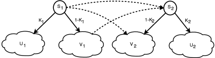
Figure 4. Splitting of successor states for weak simulations.

Let $\mathcal{M}=(S,\mathbf{P},L)$ be a DTMC and let $R\subseteq S\times S$. The relation $R$ is a weak simulation on $\mathcal{M}$ iff for all $s_{1},s_{2}$ with $s_{1}\mathrel{R}s_{2}$: $L(s_{1})=L(s_{2})$ and there exist functions $\delta_{i}:S\rightarrow[0,1]$ such that:

1. (a) $v_{1}\mathrel{R}s_{2}$ for all $v_{1}\in V_{1}$, and (b) $s_{1}\mathrel{R}v_{2}$ for all $v_{2}\in V_{2}$

2. there exists a function $\Delta:S\times S\rightarrow[0,1]$ such that:

   1. $\Delta(u_{1},u_{2})>0$ implies $u_{1}\in U_{1},u_{2}\in U_{2}$ and $u_{1}\mathrel{R}u_{2}$.

   2. if $K_{1}>0$ and $K_{2}>0$ then for all states $w\in S$:

      $$K_{1}\cdot\Delta(w,U_{2})=\mathbf{P}(s_{1},w)\delta_{1}(w),\ K_{2}\cdot\Delta(U_{1},w)=\mathbf{P}(s_{2},w)\delta_{2}(w)$$

      where $K_{i}=\sum_{u_{i}\in U_{i}}\delta_{i}(u_{i})\cdot\mathbf{P}(s_{i},u_{i})$ for $i=1,2$.

3. for $u_{1}\in U_{1}$ there exists a path fragment $s_{2},w_{1},\ldots,w_{n},u_{2}$ with positive probability such that $n\geq 0$, $s_{1}\mathrel{R}w_{j}$ for $0<j\leq n$, and $u_{1}\mathrel{R}u_{2}$.

We say that $s_{2}$ weakly simulates $s_{1}$ in $\mathcal{M}$, denoted $s_{1}\precapprox_{\mathcal{M}}s_{2}$, iff there exists a weak simulation $R$ on $\mathcal{M}$ such that $s_{1}\mathrel{R}s_{2}$. Note again that the sets $U_{i},V_{i}$ in the above definition are defined according to Equation 1 with respect to the pair $(s_{1},s_{2})$ and the functions $\delta_{i}$. The functions $\delta_{i}$ can be considered as a generalisation of the characteristic function of $U_{i}$ in the sense that we may split the membership of a state to $U_{i}$ and $V_{i}$ into fragments which sum up to $1$. For example, if $\delta_{1}(s)=\frac{1}{3}$, we say that $\frac{1}{3}$ fragment of the state $s$ belongs to $U_{1}$, and $\frac{2}{3}$ fragment of $s$ belongs to $V_{1}$. Hence, $U_{i}$ and $V_{i}$ are not necessarily disjoint. Observe that $U_{i}=\emptyset$ implies that $\delta_{i}(s)=0$ for all $s\in S$. Similarly, $V_{i}=\emptyset$ implies that $\delta_{i}(s)=1$ for all $s\in S$.

Condition 3 will in the sequel be called the reachability condition. If $K_{1}>0$ and $K_{2}=0$, which implies that $U_{2}=\emptyset$ and $U_{1}\not=\emptyset$, the reachability condition guarantees that for any visible step $s_{1}\to u_{1}$ with $u_{1}\in U_{1}$, $s_{2}$ can reach a state $u_{2}$ which simulates $u_{1}$ while passing only through states simulating $s_{1}$. Assume that we have $S=\{s_{1},s_{2},u_{1}\}$ where $L(s_{1})=L(s_{2})$ and $u_{1}$ has a different labelling. There is only one transition $\mathbf{P}(s_{1},u_{1})=1$. Obviously $s_{1}\not\precapprox s_{2}$. Dropping Condition 3 would mean that $s_{1}\precapprox s_{2}$. We illustrate the use of fragments of states in the following example:

$s_{1}$[fillstyle=solid,fillcolor=yellow]$u_{1}$ $.3$ [fillstyle=solid,fillcolor=yellow]$v_{1}$ $.2$ $s_{2}$ $.5$[fillstyle=solid,fillcolor=yellow]$v_{1}$ $1$               $s_{3}$[fillstyle=solid,fillcolor=yellow]$u_{2}$ $.15$ [fillstyle=solid,fillcolor=yellow]$v_{2}$ $.1$ $s_{4}$ $.75$[fillstyle=solid,fillcolor=yellow]$v_{1}$ $.5$ $s_{5}$ $.5$[fillstyle=solid,fillcolor=yellow]$v_{2}$ $1$

[fillstyle=solid,fillcolor=yellow]$u_{1}$               [fillstyle=solid,fillcolor=yellow]$v_{1}$$q_{1}$ $1$               [fillstyle=solid,fillcolor=yellow]$u_{2}$[fillstyle=solid,fillcolor=BlueGreen]$q_{2}$ $1$               [fillstyle=solid,fillcolor=yellow]$v_{2}$$q_{3}$ $1$[fillstyle=solid,fillcolor=BlueGreen]$q_{4}$ $1$

Figure 5. A DTMC where splitting states is necessary to establish the weak simulation. In the model some states are drawn more than once.

Consider the DTMC depicted in Figure 5. For states $u_{1},u_{2},v_{1},v_{2}$, obviously the following pairs $(u_{1},u_{2}),(u_{1},v_{2}),(v_{1},v_{2})$ are in the weak simulation relation. The state $u_{2}$ cannot weakly simulate $v_{1}$. Since $v_{2}$ weakly simulates $v_{1}$, it holds that $s_{2}\precapprox s_{5}$. Similarly, from $u_{1}\precapprox v_{1}$ we can easily show that $s_{1}\precapprox s_{4}$. We observe also that $s_{2}\not\precapprox s_{3}$: $K_{1}>0$ and $K_{2}>0$ since both $s_{2}$ and $s_{3}$ have yellow (grey) successor states, but the required function $\Delta$ cannot be established since $u_{2}$ cannot weakly simulate any successor state of $s_{2}$ (which is $v_{1}$). Thus $s_{2}\not\precapprox s_{3}$.

Without considering fragments of states, we show that a weak simulation between $s_{1}$ and $s_{3}$ cannot be established. Since $s_{2}\not\precapprox s_{3}$, we must have $U_{1}=\{u_{1},v_{1},s_{2}\}$ and $V_{1}=\emptyset$. The function $\delta_{1}$ is thus defined by $\delta_{1}(u_{1})=\delta_{1}(v_{1})=\delta(s_{2})=1$ which implies that $K_{1}=1$. Now consider the successor states of $s_{3}$. Obviously $\delta_{2}(u_{2})=\delta_{2}(v_{2})=1$, which implies that $u_{2},v_{2}\in U_{2}$. We consider the following two cases:

1. The case $\delta_{2}(s_{4})=1$. In this case we have that $K_{2}=1$. A function $\Delta$ must be defined satisfying Condition 2b in Definition 2.2.3. Taking $w=s_{4}$, the following must hold: $K_{2}\cdot\Delta(U_{1},s_{4})=\mathbf{P}(s_{3},s_{4})\delta_{2}(s_{4})$. As $K_{2}=1,\mathbf{P}(s_{3},s_{4})=0.75$ and $\delta_{2}(s_{4})=1$, it follows that $\Delta(U_{1},s_{4})=0.75$. The state $s_{2}$ is the only successor of $s_{1}$ that can be weakly simulated by $s_{4}$, so $\Delta(s_{2},s_{4})=0.75$ must hold. However, the equation $K_{1}\cdot\Delta(s_{2},U_{2})=\mathbf{P}(s_{1},s_{2})\delta_{1}(s_{2})$ does not hold any more, as on the left side we have $0.75$ but on the right side we have $0.5$ instead.

2. The case $\delta_{2}(s_{4})=0$. In this case we have still $K_{2}>0$. Similar to the previous case it is easy to see that the required function $\Delta$ cannot be defined: the equation $K_{1}\cdot\Delta(s_{2},U_{2})=\mathbf{P}(s_{1},s_{2})\delta_{1}(s_{2})$ does not hold since the left side is $0$ (no states in $U_{2}$ can weakly simulate $s_{2}$) but the right side equals $0.5$.

Thus without splitting, $s_{3}$ does not weakly simulate $s_{1}$. We show it holds that $s_{1}\precapprox s_{3}$. It is sufficient to show that the relation $R=\{(s_{1},s_{3}),(u_{1},u_{2}),(v_{1},v_{2})$, $(q_{1},q_{3}),(s_{1},s_{4})$, $(u_{1},v_{1})$, $(v_{1},v_{1}),(q_{1},q_{1})$, $(s_{2},s_{5}),(s_{2},s_{4})\}$ is a weak simulation relation. By the discussions above, it is easy to verify that every pair except $(s_{1},s_{3})$ satisfies the conditions in Definition 2.2.3. We show now that the conditions hold also for the pair $(s_{1},s_{3})$. The function $\delta_{1}$ with $\delta_{1}(u_{1})=\delta_{1}(v_{1})=\delta_{1}(s_{2})=1$ is defined as above, also the sets $U_{1}=\{u_{1},v_{1},s_{2}\}$, $V_{1}=\emptyset$. The function $\delta_{2}$ is defined by: $\delta_{2}(u_{2})=\delta_{2}(v_{2})=1$ and $\delta_{2}(s_{4})=\frac{1}{3}$, which implies that $U_{2}=\{u_{2},v_{2},s_{4}\}$ and $V_{2}=\{s_{4}\}$. Thus, we have $K_{1}=1$ and $K_{2}=0.5$. Since $s_{1}\precapprox s_{4}$, Condition 1 holds trivially as $(s_{1},s_{4})\in R$. The reachability condition also holds trivially. To show that Condition 2 holds, we define the function $\Delta$ as follows: $\Delta(u_{1},u_{2})=0.3$, $\Delta(v_{1},v_{2})=0.2$ and $\Delta(s_{2},s_{4})=0.5$. We show that $K_{2}\cdot\Delta(U_{1},w)=\mathbf{P}(s_{3},w)\delta_{2}(w)$ holds for all $w\in S$. It holds that $K_{2}=0.5$. First observe that for $w\not\in U_{2}$ both sides of the equation equal $0$. Let first $w=u_{2}$ for which we have that $\mathbf{P}(s_{3},u_{2})\delta_{2}(u_{2})=0.15$. Since $\Delta(U_{1},u_{2})=0.3$, also the left side equals $0.15$. The case $w=v_{2}$ can be shown in a similar way. Now consider $w=s_{4}$. Observe that $\Delta(U_{1},s_{4})=0.5$ thus the left side equals $0.25$. The right side equals $\mathbf{P}(s_{3},s_{4})\delta_{2}(s_{4})=0.75\cdot\frac{1}{3}=0.25$ thus the equation holds. The equation $K_{1}\cdot\Delta(w,U_{2})=\mathbf{P}(s_{1},w)\delta_{1}(w)$ can be shown in a similar way. Thus $\Delta$ satisfies all the conditions, which implies that $s_{1}\precapprox s_{3}$.

Weak simulation for CTMCs is defined as follows.

[[9, 8]] Let $\mathcal{M}=(S,\mathbf{R},L)$ be a CTMC and let $R\subseteq S\times S$. The relation $R$ is a weak simulation on $\mathcal{M}$ iff for $s_{1}\mathrel{R}s_{2}$: $L(s_{1})=L(s_{2})$ and there exist functions $\delta_{i}:S\rightarrow[0,1]$ (for $i=1,2$) satisfying Equation 1 and Conditions 1 and 2 of Definition 2.2.3 and the rate condition:

1. $K_{1}\cdot\mathbf{R}(s_{1},S)\leq K_{2}\cdot\mathbf{R}(s_{2},S)$

We say that $s_{2}$ weakly simulates $s_{1}$ in $\mathcal{M}$, denoted $s_{1}\precapprox_{\mathcal{M}}s_{2}$, iff there exists a weak simulation $R$ on $\mathcal{M}$ such that $s_{1}\mathrel{R}s_{2}$. In this definition, the rate condition $\ref{ws:reachability}^{\prime}$ strengthens the reachability condition of the preceding definition. If $U_{1}\not=\emptyset$, we have that $K_{1}>0$; the rate condition then requires that $K_{2}>0$, which implies $U_{2}\not=\emptyset$. For both DTMCs and CTMCs, the defined weak simulation $\precapprox$ is a preorder [9], and is the coarsest weak simulation relation for $\mathcal{M}$.

2.2.4. Simulation up to R

For an arbitrary relation $R$ on the state space $S$ of an FPS with $s_{1}\mathrel{R}s_{2}$, we say that $s_{2}$ simulates $s_{1}$ strongly up to $R$, denoted $s_{1}\precsim_{R}s_{2}$, if $L(s_{1})=L(s_{2})$ and $\mathbf{P}(s_{1},\cdot)\sqsubseteq_{R}\mathbf{P}(s_{2},\cdot)$. Otherwise we write $s_{1}\not\precsim_{R}s_{2}$. Since only the first step is considered for $\precsim_{R}$, $s_{1}\precsim_{R}s_{2}$ does not imply $s_{1}\precsim_{\mathcal{M}}s_{2}$ unless $R$ is a strong simulation. By definition, $R$ is a strong simulation if and only if for all $s_{1}\mathrel{R}s_{2}$ it holds that $s_{1}\precsim_{R}s_{2}$. Likewise, we say that $s_{2}$ simulates $s_{1}$ weakly up to $R$, denoted by $s_{1}\precapprox_{R}s_{2}$, if there are functions $\delta_{i}$ and $U_{i},V_{i},\Delta$ as required by Definition 2.2.3 for this pair of states. Otherwise, we write $s_{1}\not\precapprox_{R}s_{2}$. Similar to strong simulation up to $R$, $s_{1}\precapprox_{R}s_{2}$ does not imply $s_{1}\precapprox_{\mathcal{M}}s_{2}$, since no conditions are imposed on pairs in $R$ different from $(s_{1},s_{2})$. Again, $R$ is a weak simulation if and only if for all $s_{1}\mathrel{R}s_{2}$ it holds that $s_{1}\precapprox_{R}s_{2}$. These conventions extend to DTMCs, CTMCs, PAs and CPAs in an obvious way. For PAs and CPAs, strong probabilistic simulation up to $R$, denoted by $\precsim^{p}_{R}$, is also defined analogously.

$s_{1}$[fillstyle=solid,fillcolor=BlueGreen]$w_{1}$ $1$ [fillstyle=solid,fillcolor=yellow]$q_{1}$ $1$           $s_{2}$[fillstyle=solid,fillcolor=BlueGreen]$w_{2}$ $1$ [fillstyle=solid]$q_{2}$ $1$

Figure 6. A simple FPS for illustrating the simulation up to $R$.

Consider the FPS in Figure 6. Let $R=\{(s_{1},s_{2}),(w_{1},w_{2})\}$. Since $L(q_{1})\neq L(q_{2})$ we have that $w_{1}\not\precsim w_{2}$. Thus, $R$ is not a strong simulation. However, $s_{1}\precsim_{R}s_{2}$, as the weight function is given by $\Delta(w_{1},w_{2})=1$. Let $R^{\prime}=\{(s_{1},s_{2})\}$, then, $s_{1}\not\precsim_{R^{\prime}}s_{2}$.

3. Maximum Flow Problems

Before introducing algorithms to decide the simulation preorder, we briefly recall the preflow algorithm [20] for finding the maximum flow over the network $\mathcal{N}=(V,E,c)$ where $V$ is a finite set of vertices, $E\subseteq V\times V$ is a set of edges, and $c:E\to\mathbb{R}_{>0}\cup\{\infty\}$ is the capacity function. $V$ contains a distinguished source vertex ${\mathord{\nnearrow}}$ and a distinguished sink vertex ${\mathord{\ssearrow}}$. We extend the capacity function to all vertex pairs: $c(v,w)=0$ if $(v,w)\not\in E$. A flow $f$ on $\mathcal{N}$ is a function $f:V\times V\to\mathbb{R}$ that satisfies:

1. $f(v,w)\leq c(v,w)$ for all $(v,w)\in V\times V$ capacity constraints

2. $f(v,w)=-f(w,v)$ for all $(v,w)\in V\times V$ antisymmetry constraint

3. $f(V,v)=0$ at vertices $v\in V\setminus\{{\mathord{\nnearrow}},{\mathord{\ssearrow}}\}$ conservation rule

The value of a flow function $f$ is given by $f({\mathord{\nnearrow}},V)$. A maximum flow is a flow of maximum value. A preflow is a function $f:V\times V\to\mathbb{R}$ satisfying Conditions 1 and 2 above, and the relaxation of Condition 3:

1. $f(V,v)\geq 0$ for all $v\in V\setminus\{{\mathord{\nnearrow}}\}$.

The excess $e(v)$ of a vertex $v$ is defined by $f(V,v)$. A vertex $v\not\in\{{\mathord{\nnearrow}},{\mathord{\ssearrow}}\}$ is called active if $e(v)>0$. Observe that if in a preflow function no vertex $v$ is active for $v\in V\setminus\{{\mathord{\nnearrow}},{\mathord{\ssearrow}}\}$, it is then also a flow function. A pair $(v,w)$ is a residual edge of $f$ if $f(v,w)<c(v,w)$. The set of residual edges with respect to $f$ is denoted by $E_{f}$. The residual capacity $c_{f}(v,w)$ of the residual edge $(v,w)$ is defined by $c(v,w)-f(v,w)$. If $(v,w)$ is not a residual edge, it is called saturated. A valid distance function (called valid labelling in [20]) $d$ is a function $V\to\mathbb{N}\cup\{\infty\}$ satisfying: $d({\mathord{\nnearrow}})=\left\lvert V\right\rvert$, $d({\mathord{\ssearrow}})=0$ and $d(v)\leq d(w)+1$ for every residual edge $(v,w)$. A residual edge $(v,w)$ is admissible if $d(v)=d(w)+1$.

Related to maximum flows are minimum cuts. A cut of a network $\mathcal{N}=(V,E,c)$ is a partition of $V$ into two disjoint sets $(X,X^{\prime})$ such that ${\mathord{\nnearrow}}\in X$ and ${\mathord{\ssearrow}}\in X^{\prime}$. The capacity of $(X,X^{\prime})$ is the sum of all capacities of edges from $X$ to $X^{\prime}$, i. e., $\sum_{v\in X,w\in X^{\prime}}c(v,w)$. A minimum cut is a cut with minimal capacity. The Maximum Flow Minimum Cut Theorem [1] states that the capacity of a minimum cut is equal to the value of a maximum flow.

The Preflow Algorithm.

We initialise the preflow $f$ by: $f(v,w)=c(v,w)$ if $v={\mathord{\nnearrow}}$ and $0$ otherwise. The distance function $d$ is initialised by: $d(v)=\left\lvert V\right\rvert$ if $v={\mathord{\nnearrow}}$ and $0$ otherwise. The preflow algorithm preserves the validity of the preflow $f$ and the distance function $d$. If there is an active vertex $v$ such that the residual edge $(v,w)$ is admissible, we push $\delta:=\min\{e(v),c_{f}(v,w)\}$ amount of flow from $v$ toward the sink along the admissible edge $(v,w)$ by increasing $f(v,w)$ (and decreasing $f(w,v)$) by $\delta$. The excesses of $v$ and $w$ are then modified accordingly by: $e(v)=e(v)-\delta$ and $e(w)=e(w)+\delta$. If $v$ is active but there are no admissible edges leaving it, one may relabel $v$ by letting $d(v):=\min\{d(w)+1\mid(v,w)\in E_{f}\}$. Pushing and relabelling are repeated until there are no active vertices left. The algorithm terminates if no such operations apply. The resulting final preflow $f$ is a maximum flow.

Feasible Flow Problem.

Let $A\subseteq E$ be a subset of edges of the network $\mathcal{N}=(V,E,c)$, and define the lower bound function $l:A\to\mathbb{R}_{>0}$ which satisfies $l(e)\leq c(e)$ for all $e\in A$. We address the feasible flow problem which consists of finding a flow function $f$ satisfying the condition: $f(e)\geq l(e)$ for all $e\in A$. We briefly show that this problem can be reduced to the maximum flow problem [1].

We can replace a minimum flow requirement on edge $v\to w$ by turning $v$ into a demanding vertex (i. e., a vertex that consumes part of its inflow) and turning $w$ into a supplying vertex (i. e., a vertex that creates some outflow ex nihilo). The capacity of edge $v\to w$ is then reduced accordingly.

Now, we are going to look for a flow-like function for the updated network. The function should satisfy the capacity constraints, and the difference between outflow and inflow in each vertex corresponds to its supply or demand, except for ${\mathord{\nnearrow}}$ and ${\mathord{\ssearrow}}$. To remove that last exception, we add an edge from ${\mathord{\ssearrow}}$ to ${\mathord{\nnearrow}}$ with capacity $\infty$.

We then apply another transformation to the updated network so that we can apply the maximum flow algorithm. We add new source and target vertices ${\mathord{\nnearrow}}^{\prime}$ and ${\mathord{\ssearrow}}^{\prime}$. For each supplying vertex $s$, we add an edge ${\mathord{\nnearrow}}^{\prime}\to s$ with the same capacity as the supply of the vertex. For each demanding vertex $d$, we add an edge $d\to{\mathord{\ssearrow}}^{\prime}$ with the same capacity as the demand of the vertex. In [1] it is shown that the original network has a feasible flow if and only if the transformed network has a flow $h$ that saturates all edges from ${\mathord{\nnearrow}}^{\prime}$ and all edges to ${\mathord{\ssearrow}}^{\prime}$. The flow $h$ necessarily is a maximum flow, and if there is an $h$, each maximum flow satisfies the requirement; therefore it can be found by the maximum flow algorithm. An example will be given in Example 5.1.1 in Section 5.

4. Algorithms for Deciding Strong Simulations

We first recall the basic algorithm to compute the largest strong simulation relation $\precsim$ in Subsection 4.1. Then, we refine this algorithm to deal with strong simulation on Markov chains in Subsection 4.2, and extend it to deal with probabilistic automata in Subsection 4.3. In Subsection 4.4 we present an algorithm for deciding strong probabilistic simulation for probabilistic automata.

4.1. Basic Algorithm to Decide Strong Simulation

The algorithm in [3], copied as $\textnormal{SimRel}_{s}$ in Algorithm 1, takes as a parameter a model, which, for now, is an FPS $\mathcal{M}$. The subscript ‘$s$’ stands for strong simulation; a very similar algorithm, namely $\textnormal{SimRel}_{w}$, will be used for weak simulation later. To calculate the strong simulation relation for $\mathcal{M}$, the algorithm starts with the initial relation $R_{1}=\{(s_{1},s_{2})\in S\times S\mid L(s_{1})=L(s_{2})\}$ which is coarser than $\precsim_{\mathcal{M}}$. In iteration $i$, it generates $R_{i+1}$ from $R_{i}$ by deleting each pair $(s_{1},s_{2})$ from $R_{i}$ if $s_{2}$ cannot strongly simulate $s_{1}$ up to $R_{i}$, i. e., $s_{1}\not\precsim_{R_{i}}s_{2}$. This proceeds until there is no such pair left, i. e., $R_{i+1}=R_{i}$. Invariantly throughout the loop it holds that $R_{i}$ is coarser than $\precsim_{\mathcal{M}}$ (i. e., $\precsim_{\mathcal{M}}$ is a sub-relation of $R_{i}$). We obtain the strong simulation preorder $\mathord{\precsim_{\mathcal{M}}}=R_{i}$, once the algorithm terminates.

Algorithm 1: Basic algorithm to decide strong simulation.

$\textnormal{SimRel}_{s}(\mathcal{M})$

1.1:  $R_{1}\leftarrow\{(s_{1},s_{2})\in S\times S\mid L(s_{1})=L(s_{2})\}$ and $i\leftarrow 0$

1.2:  repeat

1.3:        $i\leftarrow i+1$

1.4:        $R_{i+1}\leftarrow\emptyset$

1.5:        for all $(s_{1},s_{2})\in R_{i}$ do

1.6:              if $s_{1}\precsim_{R_{i}}s_{2}$ then

1.7:                    $R_{i+1}\leftarrow R_{i+1}\cup\{(s_{1},s_{2})\}$

1.8:  until $R_{i+1}=R_{i}$

1.9:  return $R_{i}$

The decisive part of the algorithm is the check in Line 6, i. e., whether $s_{1}\precsim_{R_{i}}s_{2}$. This can be answered via solving a maximum flow problem on a particular network $\mathcal{N}(\mathbf{P}(s_{1},\cdot)$, $\mathbf{P}(s_{2},\cdot),R_{i})$ constructed from $\mathbf{P}(s_{1},\cdot)$, $\mathbf{P}(s_{2},\cdot)$ and $R_{i}$. This network is the relevant part of a graph containing two copies $t\in S_{\mathord{\bot}}$ and $\overline{t}\in\overline{S_{\mathord{\bot}}}$ of each state where $\overline{S_{\mathord{\bot}}}=\{\overline{t}\mid t\in S_{\mathord{\bot}}\}$ as follows: Let ${\mathord{\nnearrow}}$ (the source) and ${\mathord{\ssearrow}}$ (the sink) be two additional vertices not contained in $S_{\mathord{\bot}}\cup\overline{S_{\mathord{\bot}}}$. For $\mu,\mu^{\prime}\in\mathit{Dist}(S)$, and a relation $R\subseteq S\times S$ we define the network $\mathcal{N}(\mu,\mu^{\prime},R)=(V,E,c)$ with the set of vertices $V=\{{\mathord{\nnearrow}},{\mathord{\ssearrow}}\}\cup\mathit{Supp}_{\mathord{\bot}}(\mu)\cup\overline{\mathit{Supp}_{\mathord{\bot}}(\mu^{\prime})}$ and the set of edges $E$ is defined by $E=\{(s,\overline{t})\mid(s,t)\in\mathrel{R_{\mathord{\bot}}}\}\cup\{({\mathord{\nnearrow}},s)\}\cup\{(\overline{t},{\mathord{\ssearrow}})\}$ where $s\in\mathit{Supp}_{\mathord{\bot}}(\mu)$ and $t\in\mathit{Supp}_{\mathord{\bot}}(\mu^{\prime})$. Recall the relation $R_{\mathord{\bot}}$ is defined by $R\cup\{({\mathord{\bot}},s)\mid s\in S_{\mathord{\bot}}\}$. The capacity function $c$ is defined as follows: $c({\mathord{\nnearrow}},s)=\mu(s)$ for all $s\in\mathit{Supp}_{\mathord{\bot}}(\mu)$, $c(\overline{t},{\mathord{\ssearrow}})=\mu^{\prime}(t)$ for all $t\in\mathit{Supp}_{\mathord{\bot}}(\mu^{\prime})$, and $c(s,\overline{t})=\infty$ for all other $(s,\overline{t})\in E$. This network is a bipartite network, since the vertices can be partitioned into two subsets $V_{1}:=\mathit{Supp}_{\mathord{\bot}}(\mu)\cup\{{\mathord{\ssearrow}}\}$ and $V_{2}:=\overline{\mathit{Supp}_{\mathord{\bot}}(\mu^{\prime})}\cup\{{\mathord{\nnearrow}}\}$ such that all edges have one endpoint in $V_{1}$ and another in $V_{2}$. Later, we will use two variations of this network: For $\gamma\in\mathbb{R}_{>0}$, we let $\mathcal{N}(\mu,\gamma\mu^{\prime},R)$ denote the network obtained from $\mathcal{N}(\mu,\mu^{\prime},R)$ by setting the capacities to the sink ${\mathord{\ssearrow}}$ to: $c(\overline{t},{\mathord{\ssearrow}})=\gamma\mu^{\prime}(t)$. For two states $s_{1},s_{2}$ of an FPS or a CTMC, we let $\mathcal{N}(s_{1},s_{2},R)$ denote the network $\mathcal{N}(\mathbf{P}(s_{1},\cdot),\mathbf{P}(s_{2},\cdot),R)$.

The following lemma expresses the crucial relationship between maximum flows and weight functions on which the algorithm is based. It is a direct extension of [3, Lemma 5.1]:

Lemma 1.

Let $S$ be a finite set of states and $R$ be a relation on $S$. Let $\mu,\mu^{\prime}\in\mathit{Dist}(S)$. Then, $\mu\sqsubseteq_{R}\mu^{\prime}$ iff the maximum flow of the network $\mathcal{N}(\mu,\mu^{\prime},R)$ has value $1$.

Proof 4.1.

As we introduced the auxiliary state ${\mathord{\bot}}$, $\mu$ and $\mu^{\prime}$ are stochastic distributions in $\mathit{Dist}(S_{\mathord{\bot}})$. The rest of the proof follows directly from [3, Lemma 5.1].

Thus we can decide $s_{1}\precsim_{R_{i}}s_{2}$ by computing the maximum flow in $\mathcal{N}(s_{1},s_{2},R_{i})$ and then check whether it has value $1$. We recall the correctness and complexity of $\textnormal{SimRel}_{s}$ which will also be used later.

Theorem 2 ([3]).

If $\textnormal{SimRel}_{s}(\mathcal{M})$ terminates, the returned relation equals $\precsim_{\mathcal{M}}$. Moreover, $\textnormal{SimRel}_{s}(\mathcal{M})$ runs in time $\mathcal{O}(n^{7}/\log n)$ and in space $\mathcal{O}(n^{2})$.

Proof 4.2.

First we show that after the last iteration (say iteration $k$), it holds that $\precsim$ is coarser than $R_{k}$: It holds that $R_{k+1}=R_{k}$, thus for all $(s_{1},s_{2})\in R_{k}$, we have that $s_{1}\precsim_{R_{k}}s_{2}$. As for all $(s_{1},s_{2})\in R_{k}\subseteq R_{1}$, we have $L(s_{1})=L(s_{2})$, $R_{k}$ is a strong simulation relation by Definition 2.2.1, thus $\precsim$ is coarser than $R_{k}$.

Now we show by induction that the loop of the algorithm invariantly ensures that $R_{i}$ is coarser than $\precsim$. Assume $i=1$. By definition of strong simulation, $s_{1}\precsim s_{2}$ implies $L(s_{1})=L(s_{2})$. Thus, the initial relation $R_{1}$ is coarser than the simulation relation $\precsim$. Now assume that $R_{i}$ is coarser than $\precsim$ for some $1\leq i<k$; we will show that also $R_{i+1}$ is coarser than $\precsim$. Pick a pair $(s_{1},s_{2})\in\mathord{\precsim}$ arbitrarily. By Definition 2.2.1, $\mathbf{P}(s_{1},\cdot)\sqsubseteq_{\precsim}\mathbf{P}(s_{2},\cdot)$, so there exists a weight function for $(\mathbf{P}(s_{1},\cdot),\mathbf{P}(s_{2},\cdot))$ with respect to $\precsim$. Inspection of Definition 2.2.1 shows that the same function is also a weight function with respect to any set coarser than $\precsim$. As $R_{i}$ is coarser than $\precsim$ by induction hypothesis, we conclude that $\mathbf{P}(s_{1},\cdot)\sqsubseteq_{R_{i}}\mathbf{P}(s_{2},\cdot)$, and from Subsection 2.2.4, $s_{1}\precsim_{R_{i}}s_{2}$. This implies that $(s_{1},s_{2})\in R_{i+1}$ by line 6 for all $s_{1}\precsim s_{2}$. Therefore, $R_{i+1}$ is coarser than $\precsim$ for all $i=1\ldots,k$.

Now we show the complexity. For one network $\mathcal{N}(s_{1},s_{2},R_{i})=(V,E,c)$, the sizes of the vertices $\left\lvert V\right\rvert$ and edges $\left\lvert E\right\rvert$ are bounded by $2n+4$ and $(n+1)^{2}+2n$, respectively. The number of edges meets the worst case bound $\mathcal{O}(n^{2})$. To the best of our knowledge, the best complexity of the flow computation for the network $G$ is $\mathcal{O}(\left\lvert V\right\rvert^{3}/\log\left\lvert V\right\rvert)=\mathcal{O}(n^{3}/\log n)$ [14, 19]. In the algorithm $\textnormal{SimRel}_{s}$, only one pair, in the worst case, is removed from $R_{i}$ in iteration $i$, which indicates that the test whether $s_{1}\precsim_{R_{i}}s_{2}$ is called $\left\lvert R_{1}\right\rvert$ times, $\left\lvert R_{1}\right\rvert-1$ times and so on. Altogether it is bounded by $\sum_{i=1}^{\left\lvert R_{1}\right\rvert}i\leq\sum_{i=1}^{n^{2}}i\in\mathcal{O}(n^{4})$. Hence, the overall time complexity amounts to $\mathcal{O}(n^{7}/\log n)$. The space complexity is $\mathcal{O}(n^{2})$ because of the representation of the transitions in $\mathcal{N}(s_{1},s_{2},R_{i})$.

4.2. An Improved Algorithm for FPSs

We first analyse the behaviour of $\textnormal{SimRel}_{s}$ in more detail. For this, we consider an arbitrary pair $(s_{1},s_{2})$, and assume that $(s_{1},s_{2})$ stays in relation $R_{1},\ldots,R_{k}$ throughout the iterations $i=1,\ldots,k$, until the pair is either found not to satisfy $s_{1}\precsim_{R_{k}}s_{2}$ or the algorithm terminates with a fix-point after iteration $k$. Then altogether the maximum flow algorithms are run $k$-times for this pair. However, the networks $\mathcal{N}(s_{1},s_{2},R_{i})$ constructed in successive iterations are very similar, and may often be identical across iterations: They differ from iteration to iteration only by deletion of some edges induced by the successive cleanup of $R_{i}$. For our particular pair $(s_{1},s_{2})$ the network might not change at all in some iterations, because the deletions from $R_{i}$ do not affect their direct successors. We are going to exploit this observation by an algorithm that reuses the already computed maximum flow, in a way that whatever happens is good: If no changes occur from $\mathcal{N}(s_{1},s_{2},R_{i-1})$ to $\mathcal{N}(s_{1},s_{2},R_{i})$, then the maximum flow is the same as the one in the previous iteration. If changes do occur, the preflow algorithm can be applied to get the new maximum flow very fast, using the maximum flow and distance function constructed in the previous iteration as a starting point.

To understand the algorithm, we look at the network $\mathcal{N}(s_{1},s_{2},R_{1})$. Let $D_{1},\ldots,D_{k}$ be pairwise disjoint subsets of $R_{1}$, which correspond to the pairs deleted from $R_{1}$ in iteration $i$, so $R_{i+1}=R_{i}\setminus D_{i}$ for $1\leq i\leq k$. Let $f_{i}^{(s_{1},s_{2})}$ denote the maximum flow of the network $\mathcal{N}(s_{1},s_{2},R_{i})$ for $1\leq i\leq k$. We sometimes omit the superscript $(s_{1},s_{2})$ in the parameters if the pair $(s_{1},s_{2})$ is clear from the context. We address the problem of checking $\left\lvert f_{i}\right\rvert=1$ for all $i=1,\ldots,k$. Our algorithm sequence of maximum flows $\textnormal{Smf}(i,\mathcal{N}(s_{1},s_{2},R_{i-1}),f_{i-1},d_{i-1},D_{i-1})$ is shown as Algorithm 2. It executes iteration $i$ of a parametric flow algorithm, where $\mathcal{N}(s_{1},s_{2},R_{i-1})$ is the network for $(s_{1},s_{2})$ and $f_{i-1}$ and $d_{i-1}$ are the flow and the distance function resulting from the previous iteration $i-1$; and $D_{i-1}$ is a set of edges that have to be deleted from $\mathcal{N}(s_{1},s_{2},R_{i-1})$ to get the current network. The algorithm returns a tuple, in which the first component is a boolean that tells whether $\left\lvert f_{i}\right\rvert=1$; it also returns the new network $\mathcal{N}(s_{1},s_{2},R_{i})$, flow $f_{i}$ and distance function $d_{i}$ to be reused in the next iteration. Smf is inspired by the parametric maximum algorithm in [18]. A variant of Smf is used in the first iteration, shown in lines 11–13.

Algorithm 2: Algorithm for a sequence of maximum flows.

$\textnormal{Smf}(i,\mathcal{N}(s_{1},s_{2},R_{i-1}),f_{i-1},d_{i-1},D_{i-1})$

2.1:  $\mathcal{N}(s_{1},s_{2},R_{i})\leftarrow\mathcal{N}(s_{1},s_{2},R_{i-1}\setminus D_{i-1})$ and $f_{i}\leftarrow f_{i-1}$ and $d_{i}\leftarrow d_{i-1}$

2.2:  for all $(u_{1},u_{2})\in D_{i-1}$ do

2.3:        $f_{i}(\overline{u_{2}},{\mathord{\ssearrow}})\leftarrow f_{i}(\overline{u_{2}},{\mathord{\ssearrow}})-f_{i}(u_{1},\overline{u_{2}})$

2.4:        $f_{i}(u_{1},\overline{u_{2}})\leftarrow 0$

2.5:  Apply the preflow algorithm to calculate the maximum flow for $\mathcal{N}(s_{1},s_{2},R_{i})$, but initialise the preflow to $f_{i}$ and the distance function to $d_{i}$.

2.6:  return $(\left\lvert f_{i}\right\rvert=1,\mathcal{N}(s_{1},s_{2},R_{i}),f_{i},d_{i})$

$\textnormal{Smf}_{\mathit{init}}(i,s_{1},s_{2},R_{i})$

2.11:  Initialise the network $\mathcal{N}(s_{1},s_{2},R_{i})$.

2.12:  Apply the preflow algorithm to calculate the maximum flow for $\mathcal{N}(s_{1},s_{2},R_{i})$.

2.13:  return $(\left\lvert f_{i}\right\rvert=1,\mathcal{N}(s_{1},s_{2},R_{i}),f_{i},d_{i})$

Algorithm 3: Improved algorithm for deciding strong simulation for FPSs.

$\textnormal{SimRel}^{\mathrm{FPS}}_{s}(\mathcal{M})$

3.1:  $R_{1}\leftarrow\{(s_{1},s_{2})\in S\times S\mid L(s_{1})=L(s_{2})\}$ and $i\leftarrow 1$

3.2:  $R_{2}\leftarrow\emptyset$

3.3:  for all $(s_{1},s_{2})\in R_{1}$ do

3.4:        $\mathit{Listener}_{(s_{1},s_{2})}$ $\leftarrow\{(u_{1},u_{2})\mid u_{1}\in{\rm Phys.~{}Rev.~{}E}(s_{1})\wedge u_{2}\in{\rm Phys.~{}Rev.~{}E}(s_{2})\wedge L(u_{1})=L(u_{2})\}$

3.5:        $(\mathit{match},\mathcal{N}(s_{1},s_{2},R_{1}),f_{1}^{(s_{1},s_{2})},d_{1}^{(s_{1},s_{2})})\leftarrow\textnormal{Smf}_{\mathit{init}}(1,s_{1},s_{2},R_{1})$

3.6:        if $\mathit{match}$ then

3.7:              $R_{2}\leftarrow R_{2}\cup\{(s_{1},s_{2})\}$

3.8:  while $R_{i+1}\not=R_{i}$ do

3.9:        $i\leftarrow i+1$

3.10:        $R_{i+1}\leftarrow\emptyset$ and $D_{i-1}\leftarrow R_{i-1}\setminus R_{i}$

3.11:        for all $(s_{1},s_{2})\in R_{i}$ do

3.12:              $D_{i-1}^{(s_{1},s_{2})}\leftarrow\emptyset$

3.13:        for all $(s_{1},s_{2})\in D_{i-1},\quad(u_{1},u_{2})\in\mathit{Listener}_{(s_{1},s_{2})}\cap R_{i-1}$ do

3.14:              $D_{i-1}^{(u_{1},u_{2})}\leftarrow D_{i-1}^{(u_{1},u_{2})}\cup\{(s_{1},s_{2})\}$

3.15:        for all $(s_{1},s_{2})\in R_{i}$ do

3.16:              $(\mathit{match},\mathcal{N}(s_{1},s_{2},R_{i}),f_{i}^{(s_{1},s_{2})},d_{i}^{(s_{1},s_{2})})$ $\qquad\qquad\qquad\leftarrow\textnormal{Smf}(i,\mathcal{N}(s_{1},s_{2},R_{i-1}),f_{i-1}^{(s_{1},s_{2})},d_{i-1}^{(s_{1},s_{2})},D_{i-1}^{(s_{1},s_{2})})$

3.17:              if $\mathit{match}$ then

3.18:                    $R_{i+1}\leftarrow R_{i+1}\cup\{(s_{1},s_{2})\}$

3.19:  return $R_{i}$

This algorithm for sequence of maximum flow problems is called in an improved version of $\textnormal{SimRel}_{s}$ shown as Algorithm 3. Lines 2–7 contain the first iteration, very similar to the first iteration of Algorithm 1 (lines 4–7). At line 4 we prepare for later iterations the set

$$\mathit{Listener}_{(s_{1},s_{2})}=\{(u_{1},u_{2})\mid u_{1}\in{\rm Phys.~{}Rev.~{}E}(s_{1})\wedge u_{2}\in{\rm Phys.~{}Rev.~{}E}(s_{2})\wedge L(u_{1})=L(u_{2})\}\quad,$$

where ${\rm Phys.~{}Rev.~{}E}(s)=\{t\in S\mid\mathbf{P}(t,s)>0\}$. This set contains all pairs $(u_{1},u_{2})$ such that the network $\mathcal{N}(u_{1},u_{2},R_{1})$ contains the edge $(s_{1},\overline{s_{2}})$. Iteration $i$ (for $i>1$) of the loop (lines 10–18) calculates $R_{i+1}$ from $R_{i}$. In lines 11–14, we collect edges that should be removed from $\mathcal{N}(u_{1},u_{2},R_{i-1})$ in the sets $D_{i-1}^{(u_{1},u_{2})}$. At line 16, the algorithm Smf constructs the maximum flow for parameters using information from iteration $i-1$. It uses the set $D_{i-1}^{(s_{1},s_{2})}$ to update the network $\mathcal{N}(s_{1},s_{2},R_{i-1})$, flow $f_{i-1}$, a distance function $d_{i-1}$; then it constructs the maximum flow $f_{i}$ for the network $\mathcal{N}(s_{1},s_{2},R_{i})$. If Smf returns true, $(s_{1},s_{2})$ is inserted into $R_{i+1}$ and survives this iteration (line 18).

Consider the algorithm Smf and assume that $i>1$. At lines 1–4, we remove the edges $D_{i-1}$ from the network $\mathcal{N}(s_{1},s_{2},R_{i-1})$ and generate the preflow $f_{i}$ based on the flow $f_{i-1}$, which is the maximum flow of the network $\mathcal{N}(s_{1},s_{2},R_{i-1})$, by

1. setting $f_{i}(u_{1},\overline{u_{2}})=0$ for all deleted edges $(u_{1},u_{2})\in D_{i-1}$, and

2. reducing $f_{i}(\overline{u_{2}},{\mathord{\ssearrow}})$ such that the preflow $f_{i}$ becomes consistent with the (relaxed) flow conservation rule.

The excess $e(v)$ is increased if there exists $(v,w)\in D_{i-1}$ such that $f_{i-1}(v,w)>0$, and unchanged otherwise. Hence, $f_{i}$ after line 4 is a preflow. The distance function $d_{i-1}=d_{i}$ is still valid for this preflow, since removing the set of edges $D_{i-1}$ does not introduce new residual edges. This guarantees that, at line 5, the preflow algorithm finds a maximum flow over the network $\mathcal{N}(s_{1},s_{2},R_{i})$. In line 6, Smf returns whether the flow has value 1 together with information to be reused in the next iteration. (If $\left\lvert f_{k}\right\rvert<1$ at some iteration $k$, then $\left\lvert f_{j}\right\rvert<1$ for all iterations $j\geq k$ because deleting edges does not increase the maximum flow. In that case, it would be sufficient to return $\mathbf{false}$.) We prove the correctness and complexity of the algorithm Smf:

Lemma 3.

Let $(s_{1},s_{2})\in R_{1}$. Then, $\textnormal{Smf}_{\mathit{init}}$ returns true iff $s_{1}\precsim_{R_{1}}s_{2}$. For some $i>1$, let $\mathcal{N}(s_{1},s_{2},R_{i-1})$, $f_{i-1}$, and $d_{i-1}$ be as returned by some earlier call to Smf or $\textnormal{Smf}_{\mathit{init}}$. Let $D_{i-1}=(R_{i-1}\setminus R_{i})\cap(\mathit{post}(s_{1})\times\mathit{post}(s_{2}))$ be the set of edges that will be removed from the network $\mathcal{N}(s_{1},s_{2},R_{i-1})$ during the $(i-1)$th call of Smf. Then, the $(i-1)$th call of Smf returns true iff $s_{1}\precsim_{R_{i}}s_{2}$.

Proof 4.3.

By Lemma 1, $\textnormal{Smf}_{\mathit{init}}$ returns true iff $|f_{1}|=1$, which is equivalent to $s_{1}\precsim_{R_{1}}s_{2}$. Let $i>1$. As discussed, at the beginning of line 5, the function $f_{i-1}$ is a flow (thus a preflow) with value 1, and the distance function $d_{i-1}$ is a valid distance function. It follows directly from the correctness of the preflow algorithm [2] that after line 5, $f_{i}$ is a maximum flow for $\mathcal{N}(s_{1},s_{2},R_{i})$. Thus, Smf returns true (i.e. $|f_{i}|=1$) which is equivalent to $s_{1}\precsim_{R_{i}}s_{2}$.

Lemma 4.

Consider the pair $(s_{1},s_{2})$ and assume that $\left\lvert\mathit{post}(s_{1})\right\rvert\leq\left\lvert\mathit{post}(s_{2})\right\rvert$. All calls to $\textnormal{Smf}(i,\mathcal{N}(s_{1},s_{2},\cdot),\cdots)$ related to $(s_{1},s_{2})$ together run in time $\mathcal{O}(\left\lvert\mathit{post}(s_{1})\right\rvert\left\lvert\mathit{post}(s_{2})\right\rvert^{2})$.

Proof 4.4.

In the bipartite network $\mathcal{N}(s_{1},s_{2},R_{1})$, the set of vertices are partitioned into subsets $V_{1}=\mathit{post}(s_{1})\cup\{{\mathord{\ssearrow}}\}$ and $V_{2}=\mathit{post}(s_{2})\cup\{{\mathord{\nnearrow}}\}$ as described in Section 4.1. Generating the initial network (line 11) takes time in $\mathcal{O}(\left\lvert V_{1}\right\rvert\left\lvert V_{2}\right\rvert)$. In our sequence of maximum flow problems, the number of (nontrivial) iterations, denoted by $k$, is bounded by the number of edges, i. e., $k\leq\left\lvert E\right\rvert\leq\left\lvert V_{1}\right\rvert\left\lvert V_{2}\right\rvert-1$. We split the work being done by all calls to $\textnormal{Smf}(i,\mathcal{N}(s_{1},s_{2},\cdot),\ldots)$ together with the initial call to the preflow algorithm (line 12 and line 5) into edge deletions, relabels, non-saturating pushes, saturating pushes. (A non-saturating push along an edge $(u,v)$ moves all excess at $u$ to $v$; by such a push, the number of active nodes never increases.)

All edge deletions take time proportional to $\sum_{i=1}^{k}\left\lvert D_{i}\right\rvert$, which is less than the number of edges in the network. Therefore, edge deletions take time $\mathcal{O}(|V_{1}||V_{2}|)$. For all $v\in V$, it holds that $d_{i+1}(v)=d_{i}(v)$, i.e., the labelling function at the beginning of iteration $i+1$ is the same as the labelling function at the end of iteration $i$.

We discuss the time for relabelling and saturating pushes [2]. For a bipartite network, the distance of the source can be initialised to $d({\mathord{\nnearrow}})=2\left\lvert V_{1}\right\rvert$ instead of $\left\lvert V\right\rvert$, and $d(v)$ never grows above $4\left\lvert V_{1}\right\rvert$ for all $v\in V$. For $v\in V$, let $I(v)$ denote the set of nodes containing $w$ such that either $(v,w)\in E$ or $(w,v)\in E$. Intuitively, it represents edges which could be admissible leaving $v$. The time for relabel operations with respect to node $v$ is thus $(4\left\lvert V_{1}\right\rvert)|I(v)|$. Altogether, this gives the time for all relabel operations: $\sum_{v\in V}((4\left\lvert V_{1}\right\rvert)|I(v)|)\in\mathcal{O}(\left\lvert V_{1}\right\rvert\left\lvert E\right\rvert)$. Between two consecutive saturating pushes on $(v,w)$, the distances $d(v)$ and $d(w)$ must increase by $2$. Thus, the number of saturating pushes on edge $(v,w)$ is bounded by $4\left\lvert V_{1}\right\rvert$. Summing over all edges, the work for saturating pushes is bounded by $\mathcal{O}(\left\lvert V_{1}\right\rvert\left\lvert E\right\rvert)$.

Now we discuss the analysis of the number of non-saturating pushes, which is very similar to the proof of Theorem 2.2 in [22] where Max-d version of the algorithm is used. Assume that in iteration $l\leq k$ of Smf, the last relabelling action occurs. In the Max-d version [22], always the active node with the highest label is selected, and once an active node is selected, the excess of this node is pushed until it becomes $0$. This implies that, between any two relabel operations, there are at most $n$ active nodes processed (otherwise the algorithm terminates and we get the maximum flow). Also observe that at each time an active node is selected, at most one non-saturating push can occur, which implies that there are at most $n$ non-saturating pushes between node label increases. Since $d_{i}(v)$ is bounded by $4|V_{1}|$, the number of relabels altogether is bounded by $\mathcal{O}(|V_{1}||V|)$. Thus, the number of non-saturating pushes before the iteration $l$ is bounded by $\mathcal{O}(|V_{1}||V|^{2})$. Since the distance function does not change after iteration $l$ any more, inside any of the iterations $l^{\prime}\geq l$, there are again at most $n-1$ non-saturating pushes. Hence, the number of non-saturating pushes is bounded by $|V_{1}||V|^{2}+(k+1-l)(|V|-1)\in\mathcal{O}(|V_{1}||V|^{2}+k|V|)$. Since $k\leq|V_{1}||V_{2}|-1$, and $|V|\leq 2|V_{2}|$, thus, the overall time complexity amounts to $\mathcal{O}(|V_{1}||V_{2}|^{2})=\mathcal{O}(\left\lvert\mathit{post}(s_{1})\right\rvert\left\lvert\mathit{post}(s_{2})\right\rvert^{2})$ as required.

Now we give the correctness and complexity of the algorithm SimRel for FPSs:

Theorem 5.

If $\textnormal{SimRel}^{\mathrm{FPS}}_{s}(\mathcal{M})$ terminates, the returned relation equals $\precsim_{\mathcal{M}}$.

Proof 4.5.

By Lemma 3, $\textnormal{Smf}_{\mathit{init}}(i,s_{1},s_{2},R_{1})$ returns true in iteration $i=1$ iff $s_{1}\precsim_{R_{1}}s_{2}$; $\textnormal{Smf}(i,\mathcal{N}(s_{1},s_{2},R_{i-1}),\ldots)$ returns true in iteration $i>1$ iff $s_{1}\precsim_{R_{i}}s_{2}$. The rest of the correctness proof is the same as the proof of Theorem 2.

Theorem 6.

The algorithm $\textnormal{SimRel}^{\mathrm{FPS}}_{s}(\mathcal{M})$ runs in time $\mathcal{O}(m^{2}n)$ and in space $\mathcal{O}(m^{2})$. If the fanout is bounded by a constant, it has complexity $\mathcal{O}(n^{2})$, both in time and space.

Proof 4.6.

We first show the space complexity. In most cases, it is enough to store information from the previous iteration until the corresponding structure for the current iteration is calculated. The size of the set $\mathit{Listener}_{(s_{1},s_{2})}$ is bounded by $\left\lvert{\rm Phys.~{}Rev.~{}E}(s_{1})\right\rvert\left\lvert{\rm Phys.~{}Rev.~{}E}(s_{2})\right\rvert$ where ${\rm Phys.~{}Rev.~{}E}(s)=\{t\in S\mid\mathbf{P}(t,s)>0\}$. Summing over all $(s_{1},s_{2})$, we get $\sum_{s_{1}\in S}\sum_{s_{2}\in S}\left\lvert{\rm Phys.~{}Rev.~{}E}(s_{1})\right\rvert\left\lvert{\rm Phys.~{}Rev.~{}E}(s_{2})\right\rvert=m^{2}$. Assume we run iteration $i$. For every pair $(s_{1},s_{2})$, we generate the set $D_{i-1}^{(s_{1},s_{2})}$ and the network $\mathcal{N}(s_{1},s_{2},R_{i})$ together with $f_{i}$ and $d_{i}$. Obviously, the size of $D_{i-1}^{(s_{1},s_{2})}$ is bounded by $\left\lvert\mathit{post}(s_{1})\right\rvert\left\lvert\mathit{post}(s_{2})\right\rvert$. Summing over all $(s_{1},s_{2})$, we get the bound $\mathcal{O}(m^{2})$. The number of edges of the network $\mathcal{N}(s_{1},s_{2},R_{1})$ (together with $f_{i}$ and $d_{i}$) is in $\mathcal{O}(\left\lvert\mathit{post}(s_{1})\right\rvert\left\lvert\mathit{post}(s_{2})\right\rvert)$. Summing over all $(s_{1},s_{2})$ yields a memory consumption in $\mathcal{O}(m^{2})$ again. Hence, the overall space complexity is $\mathcal{O}(m^{2})$.

Now we show the time complexity. We observe that a pair $(s_{1},s_{2})$ belongs to $D_{i}$ in at most one iteration. Therefore, the time needed in lines 11–14 in all iterations together is bounded by the size of all sets $\mathit{Listener}_{(s_{1},s_{2})}$, which is $\mathcal{O}(m^{2})$. We analyse the time needed for all calls to the algorithm Smf. Recall that the fanout $g$ equals $\max_{s\in S}\left\lvert\mathit{post}(s)\right\rvert$, and therefore $\left\lvert\mathit{post}(s_{i})\right\rvert\leq g$ for $i=1,2$. By Lemma 4, the complexity attributed to the pair $(s_{1},s_{2})$ is bounded by $\mathcal{O}(g\left\lvert\mathit{post}(s_{1})\right\rvert\left\lvert\mathit{post}(s_{2})\right\rvert)$. Taking the sum over all possible pairs, we get the bound $gm^{2}\in\mathcal{O}(m^{2}n)$. If $g$ is bounded by a constant, we have $m\leq gn$, and the time complexity is $gm^{2}\leq g^{3}n^{2}\in\mathcal{O}(n^{2})$. In this case the space complexity is also $\mathcal{O}(n^{2})$.

Strong Simulation for Markov Chains.

We now consider DTMCs and CTMCs. Since each DTMC is a special case of an FPS the algorithm $\textnormal{SimRel}^{\mathrm{FPS}}_{s}$ applies directly.

Let $\mathcal{M}=(S,\mathbf{R},L)$ be a CTMC. Recall that $s\precsim_{\mathcal{M}}s^{\prime}$ holds if $s\precsim_{emb(\mathcal{M})}s^{\prime}$ in the embedded DTMC, and $s^{\prime}$ is faster than $s$. We can ensure the additional rate condition by incorporating it into the initial relation $R$. More precisely, initially $R$ contains only those pair $(s,s^{\prime})$ such that $L(s)=L(s^{\prime})$, and that the state $s^{\prime}$ is faster than $s$, i. e., we replace line 1 of the algorithm by

$$R_{1}\leftarrow\{(s_{1},s_{2})\in S\times S\mid L(s_{1})=L(s_{2})\wedge\mathbf{R}(s_{1},S)\leq\mathbf{R}(s_{2},S)\}$$

to ensure the additional rate condition of Definition 2.2.1. In the refinement steps afterwards, only the weight function conditions need to be checked with respect to the current relation in the embedded DTMC. Thus, we arrive at an algorithm for CTMCs with the same time and space complexity as for FPSs.

Consider the CTMC in the left part of Figure 7 (it has 10 states). Consider the pair $(s_{1},s_{2})\in R_{1}$. The network $\mathcal{N}(s_{1},s_{2},R_{1})$ is depicted on the right of the figure. Assume that we get the maximum flow $f_{1}$ which sends $\frac{1}{2}$ amount of flow along the path ${\mathord{\nnearrow}},u_{2},\overline{u_{4}},{\mathord{\ssearrow}}$ and $\frac{1}{2}$ amount of flow along ${\mathord{\nnearrow}},u_{1},\overline{u_{3}},{\mathord{\ssearrow}}$. Hence, the check for $(s_{1},s_{2})$ is successful in the first iteration. The checks for the pairs $(u_{1},u_{3})$, $(u_{1},u_{4})$ and $(u_{2},u_{3})$ are also successful in the first iteration. However, the check for the pair $(u_{2},u_{4})$ fails, as the probability to go from $u_{4}$ to $q_{3}$ in the embedded DTMC is $\frac{2}{5}$, while the probability to go from $u_{2}$ to $q_{1}$ in the embedded DTMC is $1$.

$s_{1}$$u_{1}$ $1$ $u_{2}$ $1$ [fillstyle=solid,fillcolor=yellow]$q_{1}$ $2$       $s_{2}$$u_{3}$ $2$ [fillstyle=solid,fillcolor=yellow]$q_{2}$ $3$ $u_{4}$ $2$ [fillstyle=solid,fillcolor=yellow]$q_{3}$ $2$ [fillstyle=solid,fillcolor=BlueGreen]$x_{1}$ $3$              

Figure 7. A CTMC example and its network $\mathcal{N}(s_{1},s_{2},R_{1})$.

In the second iteration, the network $\mathcal{N}(s_{1},s_{2},R_{2})$ is obtained from $\mathcal{N}(s_{1},s_{2},R_{1})$ by deleting the edge $(u_{2},\overline{u_{4}})$. In $\mathcal{N}(s_{1},s_{2},R_{2})$, the flows on $(u_{2},\overline{u_{4}})$ and on $(\overline{u_{4}},{\mathord{\ssearrow}})$ are set to $0$, and the vertex $u_{2}$ has a positive excess $\frac{1}{2}$. Applying the preflow algorithm, we push the excess from $u_{2}$, along $\overline{u_{3}},u_{1},\overline{u_{4}}$ to ${\mathord{\ssearrow}}$. We get a maximum flow $f_{2}$ for $\mathcal{N}(s_{1},s_{2},R_{2})$ which sends $\frac{1}{2}$ amount of flow along the path ${\mathord{\nnearrow}},u_{2},\overline{u_{3}},{\mathord{\ssearrow}}$ and $\frac{1}{2}$ amount of flow along ${\mathord{\nnearrow}},u_{1},\overline{u_{4}},{\mathord{\ssearrow}}$. Hence, the check for $(s_{1},s_{2})$ is also successful in the second iteration. Once the fix-point is reached, $R$ still contains $(s_{1},s_{2})$.

4.3. Strong Simulation for Probabilistic Automata

In this subsection we present algorithms for deciding strong simulations for PAs and CPAs. It takes the skeleton of the algorithm for FPSs: it starts with a relation $R$ which is coarser than $\precsim$, and then refines $R$ until $\precsim$ is achieved. In the refinement loop, a pair $(s,s^{\prime})$ is eliminated from the relation $R$ if the corresponding strong simulation conditions are violated with respect to the current relation. For PAs, this means that there exists an $\alpha$-successor distribution $\mu$ of $s$, such that for all $\alpha$-successor distribution $\mu^{\prime}$ of $s^{\prime}$, we cannot find a weight function for $(\mu,\mu^{\prime})$ with respect to the current relation $R$.

Let $\mathcal{M}=(S,Act,\mathbf{P},L)$ be a PA. We aim to extend Algorithm 3 to determine the strong simulation on PAs. For a pair $(s_{1},s_{2})$, assume that $L(s_{1})=L(s_{2})$ and that $\mathit{Act}(s_{1})\subseteq\mathit{Act}(s_{2})$, which is guaranteed by the initialisation. We consider line 17, which checks the condition $\mathbf{P}(s_{1},\cdot)\sqsubseteq_{R_{i}}\mathbf{P}(s_{2},\cdot)$ using Smf. By Definition 1 of strong simulation for PAs, we should instead check the condition

$$\forall\alpha\in\mathit{Act}.\ \forall s_{1}\xrightarrow{\alpha}\mu_{1}.\ \exists s_{2}\xrightarrow{\alpha}\mu_{2}\text{ with }\mu_{1}\sqsubseteq_{R_{i}}\mu_{2}$$ (2)

Recall the condition $\mu_{1}\sqsubseteq_{R_{i}}\mu_{2}$ is true iff the maximum flow of the network $\mathcal{N}(\mu_{1},\mu_{2},R_{i})$ has value one. Sometimes, we write $\mathcal{N}(s_{1},\alpha,\mu_{1},s_{2},\mu_{2},R_{i})$ to denote the network $\mathcal{N}(\mu_{1},\mu_{2},R_{i})$ associated with the pair $(s_{1},s_{2})$ with respect to action $\alpha$.

Our first goal is to extend Smf to check Condition 2 for a fixed action $\alpha$ and $\alpha$-successor distribution $\mu_{1}$ of $s_{1}$. To this end, we introduce a list $\mathit{Sim}^{(s_{1},\alpha,\mu_{1},s_{2})}$ that contains all potential candidates of $\alpha$-successor distributions of $s_{2}$ which could be used to establish the condition $\mu_{1}\sqsubseteq_{R}\mu_{2}$ for the relation $R$ considered. The set $\mathit{Sim}^{(s_{1},\alpha,\mu_{1},s_{2})}$ is represented as a list. This and some subsequent notations are similar to those used by Baier et al. in [3]. We use the function head$(\cdot)$ to read the first element of a list; tail$(\cdot)$ to read all but the first element of a list; and empty$(\cdot)$ to check whether a list is empty. As long as the network for a fixed candidate $\mu_{2}=\mathbf{head}(\mathit{Sim}^{(s_{1},\alpha,\mu_{1},s_{2})})$ allows a flow of value $1$ over the iterations, we stick to it, and we can reuse the flow and distance function from previous iterations. If by deleting some edges from $\mathcal{N}(\mu_{1},\mu_{2},R)$, its flow value falls below 1, we delete $\mu_{2}$ from $\mathit{Sim}^{(s_{1},\alpha,\mu_{1},s_{2})}$ and pick the next candidate.

Algorithm 4: Subroutine to calculate whether $s_{1}\precsim_{R_{i}}s_{2}$, as far as $s_{1}\xrightarrow{\alpha}\mu_{1}$ is concerned. The parameter $Sim$ denotes the subsets of $\alpha$-successor distributions of $s_{2}$ serving as candidates for possible $\mu_{2}$.

$\textnormal{ActSmf}(i,Sim_{i-1},\mathcal{N}(\mu_{1},\mu_{2},R_{i-1}),f_{i-1},d_{i-1},D_{i-1})$

4.1:  $Sim_{i}\leftarrow Sim_{i-1}$

4.2:  $(\mathit{match},\mathcal{N}(\mu_{1},\mu_{2},R_{i}),f_{i},d_{i})\leftarrow\textnormal{Smf}(i,\mathcal{N}(\mu_{1},\mu_{2},R_{i-1}),f_{i-1},d_{i-1},D_{i-1})$

4.3:  if $\mathit{match}$ then

4.4:        return $(\mathbf{true},Sim_{i},\mathcal{N}(\mu_{1},\mu_{2},R_{i}),f_{i},d_{i})$

4.5:  $Sim_{i}\leftarrow\mathbf{tail}(Sim_{i})$

4.6:  while $\neg\mathbf{empty}(Sim_{i})$ do

4.7:        $\mu_{2}\leftarrow\mathbf{head}(Sim_{i})$

4.8:        $(\mathit{match},\mathcal{N}(\mu_{1},\mu_{2},R_{i}),f_{i},d_{i})\leftarrow\textnormal{Smf}_{\mathit{init}}(i,\mu_{1},\mu_{2},R_{i})$

4.9:        if $\mathit{match}$ then

4.10:              return $(\mathbf{true},Sim_{i},\mathcal{N}(\mu_{1},\mu_{2},R_{i}),f_{i},d_{i})$

4.11:        $Sim_{i}\leftarrow\mathbf{tail}(Sim_{i})$

4.12:  return $(\mathbf{false},\emptyset,\mathit{NIL},\mathit{NIL},\mathit{NIL})$

$\textnormal{ActSmf}_{\mathit{init}}(i,\mu_{1},Sim_{i},R_{i})$

  4.1: goto line 6

The algorithm ActSmf, shown as Algorithm 4, implements this. It has to be called for each pair $(s_{1},s_{2})$ and each successor distribution $s_{1}\xrightarrow{\alpha}\mu_{1}$ of $s_{1}$. It takes as input the list of remaining candidates $\mathit{Sim}_{i-1}^{(s_{1},\alpha,\mu_{1},s_{2})}$, the information from the previous iteration (the network $\mathcal{N}(\mu_{1},\mu_{2},R_{i-1})$, flow $f_{i-1}$, and distance function $d_{i-1}$), and the set of edges that have to be deleted from the old network $D_{i-1}$.

Lemma 7.

Let $(s_{1},s_{2})\in R_{1}$, $\alpha\in Act(s_{1})$, and $\mu_{1}$ such that $s_{1}\xrightarrow{\alpha}\mu_{1}$. Let $Sim_{1}=\mathit{Steps}_{\alpha}(s_{2})$. Then $\textnormal{ActSmf}_{\mathit{init}}$ returns true iff $\exists\mu_{2}\text{ with }s_{2}\xrightarrow{\alpha}\mu_{2}\wedge\mu_{1}\sqsubseteq_{R_{1}}\mu_{2}$. For some $i>1$, let $Sim_{i-1}$, $\mathcal{N}(\mu_{1},\mu_{2},R_{i-1})$, $f_{i-1}$ and $d_{i-1}$ be as returned by some earlier call to ActSmf or $\textnormal{ActSmf}_{\mathit{init}}$. Let $D_{i-1}=(R_{i-1}\setminus R_{i})\cap(\mathit{Supp}(\mu_{1})\times\mathit{Supp}(\mu_{2}))$ be the set of edges that will be removed from the network during the $(i-1)$th call of ActSmf. Then, the $(i-1)$th call of algorithm ActSmf returns true iff: $\exists\mu_{2}\text{ with }s_{2}\xrightarrow{\alpha}\mu_{2}\wedge\mu_{1}\sqsubseteq_{R_{i}}\mu_{2}$.

Proof 4.7.

Once Smf returns false because the maximum flow for the current candidate $\mu_{2}$ has value $<1$, it will never become a candidate again, as edge deletions cannot lead to increased flow. The correctness proof is then the same as the proof of Lemma 3.

The algorithm $\textnormal{SimRel}^{\mathrm{PA}}_{s}$ for deciding strong simulation for PAs is presented as Algorithm 5. During the initialisation (lines 1–6, intermixed with iteration 1 in lines 7–9), for $(s_{1},s_{2})\in R_{1}$ and $s_{1}\xrightarrow{\alpha}\mu_{1}$, the list $Sim_{1}^{(s_{1},\alpha,\mu_{1},s_{2})}$ is initialised to $\mathit{Steps}_{\alpha}(s_{2})$ (line 6), as no $\alpha$-successor distribution can be excluded as a candidate a priori. As in $\textnormal{SimRel}^{\mathrm{FPS}}_{s}$, the set $\mathit{Listener}_{(s_{1},s_{2})}$ for $(s_{1},s_{2})$ is introduced which contains tuples $(u_{1},\alpha,\mu_{1},u_{2},\mu_{2})$ such that the network $\mathcal{N}(u_{1},\alpha,\mu_{1},u_{2},\mu_{2},R_{1})$ contains the edge $(s_{1},\overline{s_{2}})$.

Algorithm 5: Algorithm for deciding strong simulation for PAs, where $arc$ denotes the associated parameter $(s_{1},\alpha,\mu_{1},s_{2},\mu_{2})$.

$\textnormal{SimRel}^{\mathrm{PA}}_{s}(\mathcal{M})$

5.1:  $R_{1}\leftarrow\{(s_{1},s_{2})\in S\times S\mid L(s_{1})=L(s_{2})\wedge Act(s_{1})\subseteq Act(s_{2})\}$ and $i\leftarrow 1$

5.2:  $R_{2}\leftarrow\emptyset$

5.3:  for all $(s_{1},s_{2})\in R_{1}$ do

5.4:        $\mathit{Listener}_{(s_{1},s_{2})}$ $\leftarrow\{(u_{1},\alpha,\mu_{1},u_{2},\mu_{2})\mid$ $L(u_{1})=L(u_{2})\wedge u_{1}\xrightarrow{\alpha}\mu_{1}\wedge u_{2}\xrightarrow{\alpha}\mu_{2}$ $\mbox{}\wedge\mu_{1}(s_{1})>0\wedge\mu_{2}(s_{2})>0\}$

5.5:        for all $\alpha\in Act(s_{1}),\quad\mu_{1}\in\mathit{Steps}_{\alpha}(s_{1})$ do

5.6:              $\mathit{Sim}_{1}^{(s_{1},\alpha,\mu_{1},s_{2})}\leftarrow\mathit{Steps}_{\alpha}(s_{2})$

5.7:              $(\mathit{match}_{\alpha,\mu_{1}},\mathit{Sim}_{1}^{(s_{1},\alpha,\mu_{1},s_{2})},\mathcal{N}(s_{1},\alpha,\mu_{1},s_{2},\mu_{2},R_{1}),f_{1}^{arc},d_{1}^{arc})$ $\qquad\qquad\qquad\leftarrow\textnormal{ActSmf}_{\mathit{init}}(1,\mu_{1},\mathit{Sim}_{1}^{(s_{1},\alpha,\mu_{1},s_{2})},R_{1})$

5.8:        if $\bigwedge_{\alpha\in Act(s_{1})}\bigwedge_{\mu_{1}\in\mathit{Steps}_{\alpha}(s_{1})}\mathit{match}_{\alpha,\mu_{1}}$ then

5.9:              $R_{2}\leftarrow R_{2}\cup\{(s_{1},s_{2})\}$

5.10:  while $R_{i+1}\not=R_{i}$ do

5.11:        $i\leftarrow i+1$

5.12:        $R_{i+1}\leftarrow\emptyset$ and $D_{i-1}\leftarrow R_{i-1}\setminus R_{i}$

5.13:        for all $(s_{1},s_{2})\in R,\quad\alpha\in Act(s_{1}),\quad\mu_{1}\in\mathit{Steps}_{\alpha}(s_{1}),\quad\mu_{2}\in\mathit{Steps}_{\alpha}(s_{2})$ do

5.14:              $D_{i-1}^{(s_{1},\alpha,\mu_{1},s_{2},\mu_{2})}\leftarrow\emptyset$

5.15:        for all $(s_{1},s_{2})\in D_{i-1},\quad(u_{1},\alpha,\mu_{1},u_{2},\mu_{2})\in\mathit{Listener}_{(s_{1},s_{2})}$ do

5.16:              if $(u_{1},u_{2})\in R_{i-1}$ then

5.17:                    $D_{i-1}^{(u_{1},\alpha,\mu_{1},u_{2},\mu_{2})}\leftarrow D_{i-1}^{(u_{1},\alpha,\mu_{1},u_{2},\mu_{2})}\cup\{(s_{1},s_{2})\}$

5.18:        for all $(s_{1},s_{2})\in R$ do

5.19:              for all $\alpha\in Act(s_{1}),\quad\mu_{1}\in\mathit{Steps}_{\alpha}(s_{1})$ do

5.20:                    $(\mathit{match}_{\alpha,\mu_{1}},\mathit{Sim}_{i}^{(s_{1},\alpha,\mu_{1},s_{2})},\mathcal{N}(s_{1},\alpha,\mu_{1},s_{2},\mu_{2},R_{i}),f_{i}^{arc},d_{i}^{arc})$ $\qquad\qquad\qquad\leftarrow\textnormal{ActSmf}($ $i,\mathit{Sim}_{i-1}^{(s_{1},\alpha,\mu_{1},s_{2})},\mathcal{N}(s_{1},\alpha,\mu_{1},s_{2},\mu_{2},R_{i-1}),$ $f_{i-1}^{arc},d_{i-1}^{arc},D_{i-1}^{arc})$

5.21:              if $\bigwedge_{\alpha\in Act(s_{1})}\bigwedge_{\mu_{1}\in Steps_{\alpha}(s_{1})}\mathit{match}_{\alpha,\mu_{1}}$ then

5.22:                    $R_{i+1}\leftarrow R_{i+1}\cup\{(s_{1},s_{2})\}$

5.23:  return $R_{i}$

The main iteration starts with generating the sets $D_{i-1}^{(u_{1},\alpha,\mu_{1},u_{2},\mu_{2})}$ in lines 13–17 in a similar way as $\textnormal{SimRel}^{\mathrm{FPS}}_{s}$. Lines 19–22 check Condition 2 by calling ActSmf for each action $\alpha$ and each $\alpha$-successor distribution $\mu_{1}$ of $s_{1}$. The condition is true if and only if $match_{\alpha,\mu_{1}}$ is true for all $\alpha\in Act(s_{1})$ and $\mu_{1}\in Steps_{\alpha}(s_{1})$. In this case we insert the pair $(s_{1},s_{2})$ into $R_{i+1}$ (line 22). We give the correctness of the algorithm:

Theorem 8.

When $\textnormal{SimRel}^{\mathrm{PA}}_{s}(\mathcal{M})$ terminates, the returned relation equals $\precsim_{\mathcal{M}}$.

Proof 4.8.

The proof follows the same lines as the proof of the correctness of $\textnormal{SimRel}^{\mathrm{FPS}}_{s}$ in Theorem 5. The only new element is that we now have to quantify over the actions and successor distributions as prescribed by Definition 1. This translates to a conjunction in lines 8 and 21 of the algorithm. Exploiting Lemma 7 we get the correctness.

Now we give the complexity of the algorithm:

Theorem 9.

The algorithm $\textnormal{SimRel}^{\mathrm{PA}}_{s}(\mathcal{M})$ runs in time $\mathcal{O}(m^{2}n)$ and in space $\mathcal{O}(m^{2})$. If the fanout of $\mathcal{M}$ is bounded by a constant, it has complexity $\mathcal{O}(n^{2})$, both in time and space.

Proof 4.9.

We first consider the space complexity. We save the sets $D_{i}^{(s_{1},\alpha,\mu_{1},s_{2},\mu_{2})}$, the networks $\mathcal{N}(s_{1},\alpha,\mu_{1},s_{2},\mu_{2},R_{i})$ which are updated in every iteration, $\mathit{Listener}_{(s_{1},s_{2})}$ and the sets $\mathit{Sim}_{i}^{(s_{1},\alpha,\mu_{1},s_{2})}$. The size of the set $D_{i}^{(s_{1},\alpha,\mu_{1},s_{2},\mu_{2})}$ is in $\mathcal{O}(\left\lvert\mu_{1}\right\rvert\left\lvert\mu_{2}\right\rvert)$, which is the maximal number of edges of $\mathcal{N}(s_{1},\alpha,\mu_{1},s_{2},\mu_{2},R_{i})$. Summing over all $(s_{1},\alpha,\mu_{1},s_{2},\mu_{2})$, we get:

$$\sum_{s_{1}\in S}\sum_{\alpha\in Act(s_{1})}\sum_{\mu_{1}\in Steps_{\alpha}(s_{1})}\sum_{s_{2}\in S}\sum_{\mu_{2}\in Steps_{\alpha}(s_{2})}\left\lvert\mu_{1}\right\rvert\left\lvert\mu_{2}\right\rvert\leq m^{2}$$ (3)

Similarly, the memory needed for saving the networks has the same bound $\mathcal{O}(m^{2})$. Now we consider the set $\mathit{Listener}_{(s_{1},s_{2})}$ for the pair $(s_{1},s_{2})\in R_{1}$. Let $(u_{1},\alpha,\mu_{1},u_{2},\mu_{2})\in\mathit{Listener}_{(s_{1},s_{2})}$. Then, it holds that $s_{1}\in\mathit{Supp}(\mu_{1})$ and $s_{2}\in\mathit{Supp}(\mu_{2})$. Hence, the tuple $(u_{1},\alpha,\mu_{1},u_{2},\mu_{2})$ can be an element of $\mathit{Listener}_{(s_{1},s_{2})}$ of some arbitrary pair $(s_{1},s_{2})$ at most $\left\lvert\mu_{1}\right\rvert\left\lvert\mu_{2}\right\rvert$ times, which corresponds to the maximal number of edges between the set of nodes $\mathit{Supp}(\mu_{1})$ and $\overline{\mathit{Supp}(\mu_{2})}$ in $\mathcal{N}(s_{1},\alpha,\mu_{1},s_{2},\mu_{2},R_{1})$. Summing over all $(s_{1},\alpha,\mu_{1},s_{2},\mu_{2})$, we get that memory needed for the set $\mathit{Listener}$ is also bounded by $\mathcal{O}(m^{2})$. For each pair $(s_{1},s_{2})$ and $s_{1}\xrightarrow{\alpha}\mu_{1}$, the set $\mathit{Sim}_{1}^{(s_{1},\alpha,\mu_{1},s_{2})}$ has size $\left\lvert Steps_{\alpha}(s_{2})\right\rvert$. Summing up, this is smaller than or equal to $m^{2}$ according to Inequality 3. Hence, the overall space complexity amounts to $\mathcal{O}(m^{2})$.

Now we consider the time complexity. All initialisations (lines 1–6 of $\textnormal{SimRel}^{\mathrm{PA}}_{s}$ and the initialisations in $\textnormal{ActSmf}_{\mathit{init}}$, which calls $\textnormal{Smf}_{\mathit{init}}$) take $\mathcal{O}(m^{2})$ time. We observe that a pair $(s_{1},s_{2})$ belongs to $D_{i}$ during at most one iteration. Because of the Inequality 3, the time needed in lines 13–17 is in $\mathcal{O}(m^{2})$. The rest of the algorithm is dominated by the time needed for calling Smf in line 2 of ActSmf. By Lemma 4, the time complexity for successful and unsuccessful checks concerning the tuple $(s_{1},\alpha,\mu_{1},s_{2},\mu_{2})$ is bounded by $\mathcal{O}(g\left\lvert\mu_{1}\right\rvert\left\lvert\mu_{2}\right\rvert)$. Taking the sum over all possible tuples $(s_{1},\alpha,\mu_{1},s_{2},\mu_{2})$ we get the bound $gm^{2}$ according to Inequality 3. Hence, the complexity is $\mathcal{O}(m^{2}n)$. If the fanout $g$ is bounded by a constant, we have $m\leq gn$. Thus, the time complexity is in the order of $\mathcal{O}(n^{2})$. In this case the space complexity is also $\mathcal{O}(n^{2})$.

Remark 10.

Let $\mathcal{M}=(S,Act,\mathbf{P},L)$ be a PA, and let $k=\sum_{s\in S}\sum_{\alpha\in Act(s)}\left\lvert Steps_{\alpha}(s)\right\rvert$, called the number of transitions in [3], denote the number of all distributions in $\mathcal{M}$. The algorithm for deciding strong simulation introduced by Baier et al. has time complexity $\mathcal{O}((kn^{6}+k^{2}n^{3})/\log n)$, and space complexity $\mathcal{O}(k^{2})$. The number of distributions $k$ and the size of transitions $m$ are related by $k\leq m\leq nk$. The left equality is established if $\left\lvert\mu\right\rvert=1$ for all distributions, and the right equality is established if $\left\lvert\mu\right\rvert=n$ for all distributions.

The decision algorithm for strong simulation for CPAs can be adapted from $\textnormal{SimRel}^{\mathrm{PA}}_{s}$ in Algorithm 5 easily: Notations are extended with respect to rate functions instead of distributions in an obvious way. To guarantee the additional rate condition, we rule out successor rate functions of $s_{2}$ that violate it by replacing line 6 by:

$$\mathit{Sim}_{1}^{(s_{1},\alpha,r_{1},s_{2})}\leftarrow\{r_{2}\in Steps_{\alpha}(s_{2})\mid r_{1}(S)\leq r_{2}(S)\}.$$

For each pair $(s_{1},s_{2})$, and successor rate functions $r_{i}\in\mathit{Steps}_{\alpha}(s_{i})$ ($i=1,2$), the subroutine for checking whether $r_{1}\sqsubseteq_{R_{i}}r_{2}$ is then performed in the network $\mathcal{N}(\mu(r_{1}),\mu(r_{2}),R_{i})$. Obviously, the so obtained algorithm for CPAs has the same complexity $\mathcal{O}(m^{2}n)$.

4.4. Strong Probabilistic Simulation

The problem of deciding strong probabilistic simulation for PAs has not been tackled yet. We show that it can be computed by solving LP problems which are decidable in polynomial time [27]. In Subsection 4.4.1, we first present an algorithm for PAs. We extend the algorithm to deal with CPAs in Subsection 4.4.2.

4.4.1. Probabilistic Automata

Recall that strong probabilistic simulation is a relaxation of strong simulation in the sense that it allows combined transitions, which are convex combinations of multiple distributions belonging to equally labelled transitions. Again, the most important part is to check whether $s_{1}\precsim_{R}^{p}s_{2}$ where $R$ is the current relation. By Definition 2.2.2, it suffices to check $L(s_{1})=L(s_{2})$ and the condition:

$$\forall\alpha\in\mathit{{Act}}.\ \forall s_{1}\xrightarrow{\alpha}\mu_{1}.\ \exists s_{2}\stackrel{{\scriptstyle\alpha}}{{\leadsto}}\mu_{2}\text{ with }\mu_{1}\sqsubseteq_{R}\mu_{2}$$ (4)

However, since the combined transition involves the quantification of the constants $c_{i}\in[0,1]$, there are possibly infinitely many such $\mu_{2}$. Thus, one cannot check $\mu_{1}\sqsubseteq_{R}\mu_{2}$ for each possible candidate $\mu_{2}$. The following lemma shows that this condition can be checked by solving LP problems which are decidable in polynomial time [27, 38].

Lemma 11.

Let $\mathcal{M}=(S,Act,\mathbf{P},L)$ be a given PA, and let $R\subseteq S\times S$. Let $(s_{1},s_{2})\in R$ with $L(s_{1})=L(s_{2})$ and $Act(s_{1})\subseteq Act(s_{2})$. Then, $s_{1}\precsim_{R}^{p}s_{2}$ iff for each transition $s_{1}\xrightarrow{\alpha}\mu$, the following LP has a feasible solution:

$$\sum_{i=1}^{k}c_{i}=1$$ (5)

$$0\leq c_{i}\leq 1\qquad\forall\ i=1,\ldots,k$$ (6)

$$0\leq f_{(s,t)}\leq 1\qquad\forall(s,t)\in R_{\mathord{\bot}}$$ (7)

$$\mu(s)=\sum_{t\in R_{\mathord{\bot}}(s)}f_{(s,t)}\qquad\forall s\in S_{\mathord{\bot}}$$ (8)

$$\sum_{s\in R_{\mathord{\bot}}^{-1}(t)}f_{(s,t)}=\sum_{i=1}^{k}c_{i}\mu_{i}(t)\qquad\forall t\in S_{\mathord{\bot}}$$ (9)

where $k=\left\lvert\mathit{Steps}_{\alpha}(s_{2})\right\rvert>0$ and $\mathit{Steps}_{\alpha}(s_{2})=\{\mu_{1},\ldots,\mu_{k}\}$.

Proof 4.10.

First assume that $s_{1}\precsim_{R}^{p}s_{2}$. Let $s_{1}\xrightarrow{\alpha}\mu$. By the definition of simulation up to $R$ for strong probabilistic simulation, there exists a combined transition $s_{2}\stackrel{{\scriptstyle\alpha}}{{\leadsto}}\mu_{c}$ with $\mu\sqsubseteq_{R}\mu_{c}$. Let $\mathit{Steps}_{\alpha}(s_{2})=\{\mu_{1},\ldots,\mu_{k}\}$ where $k=\left\lvert\mathit{Steps}_{\alpha}(s_{2})\right\rvert$. Now $Act(s_{1})\subseteq Act(s_{2})$ implies $k>0$. By definition of combined transition (Definition 2.2.2), there exist constants $c_{1},\ldots,c_{k}\in[0,1]$ with $\sum_{i=1}^{k}c_{i}=1$ such that $\mu_{c}=\sum_{i=1}^{k}c_{i}\mu_{i}$. Thus Constraints 5 and 6 hold. Since $\mu\sqsubseteq_{R}\mu_{c}$, there exists a weight function $\Delta:S_{\mathord{\bot}}\times S_{\mathord{\bot}}\rightarrow[0,1]$ for $(\mu,\mu_{c})$ with respect to $R$. For every pair $(s,t)\in R_{\mathord{\bot}}$, let $f_{(s,t)}:=\Delta(s,t)$. Thus, Constraint 7 holds trivially. By Definition 2.2.1 of weight functions, it holds that (i) $\Delta(s,t)>0$ implies that $(s,t)\in R_{\mathord{\bot}}$, (ii) $\mu(s)=\sum_{t\in S_{\mathord{\bot}}}\Delta(s,t)$ for $s\in S_{\mathord{\bot}}$, and (iii) $\mu_{c}(t)=\sum_{s\in S_{\mathord{\bot}}}\Delta(s,t)$ for all $t\in S_{\mathord{\bot}}$. Observe that (i) implies that for all $(s,t)\not\in R_{\mathord{\bot}}$, we have that $\Delta(s,t)=0$. Thus, (ii) and (iii) imply Equations 8 and 9 respectively.

Now we show the other direction. Let $k=\left\lvert\mathit{Steps}_{\alpha}(s_{2})\right\rvert$ and $\mathit{Steps}_{\alpha}(s_{2})=\{\mu_{1},\ldots,\mu_{k}\}$. By assumption, for each $s_{1}\xrightarrow{\alpha}\mu$, we have a feasible solution $c_{1},\ldots,c_{k}$ and $f_{(s,t)}$ for all $(s,t)\in R_{\mathord{\bot}}$ which satisfies all of the constraints. We define $\mu_{c}=\sum_{i=1}^{k}c_{i}\mu_{i}$. By Definition 2.2.2, $\mu_{c}$ is a combined transition, thus $s_{2}\stackrel{{\scriptstyle\alpha}}{{\leadsto}}\mu_{c}$. It remains to show that $\mu\sqsubseteq_{R}\mu_{c}$. We define a function $\Delta$ as follows: $\Delta(s,t)$ equals $f_{(s,t)}$ if $(s,t)\in R_{\mathord{\bot}}$ and $0$ otherwise. With the help of Constraints 7, 8 and 9 we have that $\Delta$ is a weight function for $(\mu,\mu_{c})$ with respect to $R$, thus $\mu\sqsubseteq_{R}\mu_{c}$.

Now we are able to check Condition 4 by solving LP problems. For a PA $\mathcal{M}=(S,Act,\mathbf{P},L)$, and a relation $R\subseteq S\times S$, let $(s_{1},s_{2})\in R$ with $L(s_{1})=L(s_{2})$ and $Act(s_{1})\subseteq Act(s_{2})$. For $s_{1}\xrightarrow{{\alpha}}\mu_{1}$, we introduce a predicate $LP(s_{1},\alpha,\mu,s_{2})$ which is true iff the LP problem described as in Lemma 11 has a solution. Then, $s_{1}\precsim_{R}^{p}s_{2}$ iff the conjunction $\bigwedge_{\alpha\in{Act}(s_{1})}\bigwedge_{\mu_{1}\in\mathit{Steps}_{\alpha}(s_{1})}LP(s_{1},\alpha,\mu_{1},s_{2})$ is true. The algorithm, which is denoted by $\textnormal{SimRel}_{s}^{\mathrm{PA},p}(\mathcal{M})$, is depicted in Algorithm 6. It takes the skeleton of $\textnormal{SimRel}_{s}(\mathcal{M})$. The key difference is that we incorporate the predicate $LP(s_{1},\alpha,\mu_{1},s_{2})$ in line 7. The correctness of the algorithm $\textnormal{SimRel}_{s}^{\mathrm{PA},p}(\mathcal{M})$ can be obtained from the one of $\textnormal{SimRel}_{s}(\mathcal{M})$ together with Lemma 11. We discuss briefly the complexity. The number of variables in the LP problem in Lemma 11 is $k+\left\lvert R\right\rvert$, and the number of constraints is $1+k+\left\lvert R\right\rvert+2\left\lvert S\right\rvert\in\mathcal{O}(\left\lvert R\right\rvert)$. In iteration $i$ of $\textnormal{SimRel}_{s}^{\mathrm{PA},p}(\mathcal{M})$, for $(s_{1},s_{2})\in R_{i}$ and $s_{1}\xrightarrow{\alpha}\mu_{1}$, the corresponding LP problem is queried once. The number of iterations is in $\mathcal{O}(n^{2})$. Therefore, in the worst case, one has to solve $n^{2}\sum_{s\in S}\sum_{\alpha\in{Act}(s)}\sum_{\mu\in\mathit{Steps}_{\alpha}(s)}1\in\mathcal{O}(n^{2}m)$ many such LP problems and each of them has at most $\mathcal{O}(n^{2})$ constraints.

Algorithm 6: Algorithm for deciding strong probabilistic simulation for PAs.

$\textnormal{SimRel}_{s}^{\mathrm{PA},p}(\mathcal{M})$

6.1:  $R_{1}\leftarrow\{(s_{1},s_{2})\in S\times S\mid L(s_{1})=L(s_{2})\wedge Act(s_{1})\subseteq Act(s_{2})\}$ and $i\leftarrow 0$

6.2:  repeat

6.3:        $i\leftarrow i+1$

6.4:        $R_{i+1}\leftarrow\emptyset$

6.5:        for all $(s_{1},s_{2})\in R_{i}$ do

6.6:              for all $\alpha\in{Act}(s_{1}),\quad\mu_{1}\in\mathit{Steps}_{\alpha}(s_{1})$ do

6.7:                    $match_{\alpha,\mu_{1}}\leftarrow LP(s_{1},\alpha,\mu_{1},s_{2})$

6.8:              if $\bigwedge_{\alpha\in{Act}(s_{1})}\bigwedge_{\mu_{1}\in\mathit{Steps}_{\alpha}(s_{1})}match_{\alpha,\mu_{1}}$ then

6.9:                    $R_{i+1}\leftarrow R_{i+1}\cup\{(s_{1},s_{2})\}$

6.10:  until $R_{i+1}=R_{i}$

6.11:  return $R_{i}$

4.4.2. Continuous-time Probabilistic Automata

Now we discuss how to extend the algorithm to handle CPAs. Let $\mathcal{M}=(S,Act,\mathbf{R},L)$ be a CPA. Similar to PAs, the most important part is to check the condition $s_{1}\precsim_{R}^{p}s_{2}$ for some relation $R\subseteq S\times S$. By Definition 2.2.2, it suffices to check $L(s_{1})=L(s_{2})$ and the condition:

$$\forall\alpha\in\mathit{{Act}}.\ \forall s_{1}\xrightarrow{\alpha}r_{1}.\ \exists s_{2}\stackrel{{\scriptstyle\alpha}}{{\leadsto}}r_{2}\text{ with }\mu(r_{1})\sqsubseteq_{R}\mu(r_{2})\wedge r_{1}(S)\leq r_{2}(S)$$ (10)

Recall that for CPAs only successor rate functions with the same exit rate can be combined together. For state $s\in S$, we let $E(s):=\{r(S)\mid s\xrightarrow{\alpha}r\}$ denote the set of all possible exit rates of $\alpha$-successor rate functions of $s$. For $E\in E(s)$ and $\alpha\in{Act}(s)$, we let $\mathit{Steps}^{E}_{\alpha}(s)=\{r\in\mathit{Steps}_{\alpha}(s)\mid r(S)=E\}$ denote the set of $\alpha$-successor rate functions of $s$ with the same exit rate $E$. As for PAs, to check the condition $s_{1}\precsim_{R}^{p}s_{2}$ we resort to a reduction to LP problems.

Lemma 12.

Let $\mathcal{M}=(S,Act,\mathbf{R},L)$ be a given CPA, and let $R\subseteq S\times S$. Let $(s_{1},s_{2})\in R$ with $L(s_{1})=L(s_{2})$ and that $Act(s_{1})\subseteq Act(s_{2})$. Then, $s_{1}\precsim_{R}^{p}s_{2}$ iff for each transition $s_{1}\xrightarrow{\alpha}r$ either $r(S)=0$, or there exists $E\in E(s_{2})$ with $E\geq r(S)$ such that the following LP has a feasible solution, which consists of Constraints 5, 6, 7 of Lemma 11, and additionally:

$$r(s)=r(S)\sum_{t\in R_{\mathord{\bot}}(s)}f_{(s,t)}\qquad\forall s\in S_{\mathord{\bot}}$$ (11)

$$E\sum_{s\in R_{\mathord{\bot}}^{-1}(t)}f_{(s,t)}=\sum_{i=1}^{k}c_{i}r_{i}(t)\qquad\forall t\in S_{\mathord{\bot}}$$ (12)

where $k=\left\lvert\mathit{Steps}^{E}_{\alpha}(s)\right\rvert$ with $\mathit{Steps}^{E}_{\alpha}(s)=\{r_{1},\ldots,r_{k}\}$.

Proof 4.11.

The proof follows the same strategy as the proof of Lemma 11, in which the induced distribution of the corresponding rate function should be used.

Algorithm 7: Algorithm for deciding strong probabilistic simulation for CPAs.

$\textnormal{SimRel}_{s}^{\mathrm{CPA},p}(\mathcal{M})$

7.1:  $R_{1}\leftarrow\{(s_{1},s_{2})\in S\times S\mid L(s_{1})=L(s_{2})\wedge Act(s_{1})\subseteq Act(s_{2})\}$ and $i\leftarrow 0$

7.2:  repeat

7.3:        $i\leftarrow i+1$

7.4:        $R_{i+1}\leftarrow\emptyset$

7.5:        for all $(s_{1},s_{2})\in R_{i}$ do

7.6:              for all $\alpha\in{Act}(s_{1}),\quad r_{1}\in\mathit{Steps}_{\alpha}(s_{1}),\quad E\in E(s_{2})$ do

7.7:                    $match_{\alpha,r_{1},E}\leftarrow LP^{\prime}(s_{1},\alpha,r_{1},s_{2},E)$

7.8:              if $\bigwedge_{\alpha\in{Act}(s_{1})}\bigwedge_{r_{1}\in\mathit{Steps}_{\alpha}(s_{1})}\bigwedge_{E\in E(s_{2})}match_{\alpha,r_{1},E}$ then

7.9:                    $R_{i+1}\leftarrow R_{i+1}\cup\{(s_{1},s_{2})\}$

7.10:  until $R_{i+1}=R_{i}$

7.11:  return $R_{i}$

Now we are able to check Condition 10 by solving LP problems. For a CPA $\mathcal{M}=(S,Act,\mathbf{R},L)$, and a relation $R\subseteq S\times S$, let $(s_{1},s_{2})\in R$ with $L(s_{1})=L(s_{2})$ and $Act(s_{1})\subseteq Act(s_{2})$. For $s_{1}\xrightarrow{{\alpha}}r_{1}$, and $E\in E(s_{2})$, we introduce the predicate $LP^{\prime}(s_{1},\alpha,r_{1},s_{2},E)$ which is true iff $E\geq r_{1}(S)$ and the corresponding LP problem has a solution. Then, $s_{1}\precsim_{R}^{p}s_{2}$ iff the conjunction $\bigwedge_{\alpha\in{Act}(s_{1})}\bigwedge_{r_{1}\in\mathit{Steps}_{\alpha}(s_{2})}\bigwedge_{E\in E(s_{2})}LP^{\prime}(s_{1},\alpha,r_{1},s_{2},E)$ is true. The decision algorithm is given in Algorithm 7. As complexity we have to solve $\mathcal{O}(n^{2}m)$ LP problems and each of them has at most $\mathcal{O}(n^{2})$ constraints.

5. Algorithms for Deciding Weak Simulations

We now turn our attention to weak simulations. Similar to strong simulations, the core of the algorithm is to check whether $s_{1}\precapprox_{R}s_{2}$, i.e., $s_{2}$ weakly simulates $s_{1}$ up to the current relation $R$. As for strong simulation up to $R$, $s_{1}\precapprox_{R}s_{2}$ does not imply $s_{1}\precapprox_{\mathcal{M}}s_{2}$, since no conditions are imposed on pairs in $R$ different from $(s_{1},s_{2})$. By the definition of weak simulation, for fixed characteristic functions $\delta_{i}$ ($i=1,2$), the weight function conditions can be checked by applying maximum flow algorithms. Unfortunately, $\delta_{i}$-functions are not known a priori. Inspired by the parametric maximum flow algorithm, in this chapter, we show that one can determine whether such characteristic functions $\delta_{i}$ exist with the help of breakpoints, which can be computed by analysing a parametric network constructed out of $\mathbf{P}(s_{1},\cdot),\mathbf{P}(s_{2},\cdot)$ and $R$. We present dedicated algorithms for DTMCs in Subsection 5.1 and CTMCs in Subsection 5.2.

5.1. An Algorithm for DTMCs

Let $\mathcal{M}=(S,\mathbf{P},L)$ be a DTMC. Let $R\subseteq S\times S$ be a relation and $s_{1}\mathrel{R}s_{2}$. Whether $s_{2}$ weakly simulates $s_{1}$ up to $R$ is equivalent to whether there exist functions $\delta_{i}:S\to[0,1]$ such that the conditions in Definition 2.2.3 are satisfied. Assume that we are given the $U_{i}$-characterising functions $\delta_{i}$. In this case, $s_{1}\precapprox_{R}s_{2}$ can be checked as follows:

1. Concerning Condition 1a we check whether for all $v\in S$ with $\delta_{1}(v)<1$ it holds that $v\mathrel{R}s_{2}$. Similarly, for Condition 1b, we check whether for all $v\in S$ with $\delta_{2}(v)<1$ it holds that $s_{1}\mathrel{R}v$.

2. The reachability condition can be checked by using standard graph algorithms. In more detail, for each $u$ with $\delta_{1}(u)>0$, the condition holds if a state in $R(u)$ is reachable from $s_{2}$ via $R(s_{1})$ states.

3. Finally consider Condition 2. From the given $\delta_{i}$ functions we can compute $K_{i}$. In case of that $K_{1}>0$ and $K_{2}>0$, we need to check whether there exists a weight function for the conditional distributions ${\mathbf{P}(s_{1},\cdot)}/{K_{1}}$ and ${\mathbf{P}(s_{2},\cdot)}/{K_{2}}$ with respect to the current relation $R$. From Lemma 1, this is equivalent to check whether the maximum flow for the network constructed from $({\mathbf{P}(s_{1},\cdot)}/{K_{1}},{\mathbf{P}(s_{2},\cdot)}/{K_{2}})$ and $R$ has value $1$.

To check $s_{1}\precapprox_{R}s_{2}$, we want to check whether such $\delta_{i}$ functions exist. The difficulty is that there exist uncountably many possible $\delta_{i}$ functions. In this section, we first show that whether such $\delta_{i}$ exists can be characterised by analysing a parametric network in Subsection 5.1.1. Then, in Subsection 5.1.2, we recall the notion of breakpoints, and show that the breakpoints play a central role in the parametric networks considered: only these points need to be considered. Based on this, we present the algorithm for DTMCs in Subsection 5.1.3. An improvement of the algorithm for certain cases is reported in Subsection 5.1.4.

5.1.1. The Parametric Network $\mathcal{N}(\gamma)$

Let $\gamma\in\mathbb{R}_{\geq 0}$. Recall that $\mathcal{N}(\mathbf{P}(s_{1},\cdot),\gamma\mathbf{P}(s_{2},\cdot),R)$ is obtained from the network $\mathcal{N}(\mathbf{P}(s_{1},\cdot),\mathbf{P}(s_{2},\cdot),R)$ be setting the capacities to the sink ${\mathord{\ssearrow}}$ by: $c(\overline{t},{\mathord{\ssearrow}})=\gamma\mathbf{P}(s_{2},t)$. If $s_{1},s_{2},R$ are clear from the context, we use $\mathcal{N}(\gamma)$ to denote the network $\mathcal{N}(\mathbf{P}(s_{1},\cdot),\gamma\mathbf{P}(s_{2},\cdot),R)$ for arbitrary $\gamma\in\mathbb{R}_{\geq 0}$.

We introduce some notations. We focus on a particular pair $(s_{1},s_{2})\in R$, where $R$ is the current relation. We partition the set $\mathit{post}(s_{i})$ into $MU_{i}$ (for: must be in $U_{i}$) and $PV_{i}$ (for: potentially in $V_{i}$). The set $PV_{1}$ consists of those successors of $s_{1}$ which can be either put into $U_{1}$ or $V_{1}$ or both: $PV_{1}=\mathit{post}(s_{1})\cap R^{-1}(s_{2})$. The set $MU_{1}$ equals $\mathit{post}(s_{1})\backslash PV_{1}$, which consists of the successor states which can only be placed in $U_{1}$. The sets $PV_{2}$ and $MU_{2}$ are defined similarly by: $PV_{2}=\mathit{post}(s_{2})\cap R(s_{1})$ and $MU_{2}=\mathit{post}(s_{2})\backslash PV_{2}$. Obviously, $\delta_{i}(u)=1$ for $u\in MU_{i}$ for $i=1,2$.

$s_{1}$[fillstyle=solid,fillcolor=yellow]$u_{1}$ $\frac{1}{4}$ $o_{1}$ $\frac{1}{2}$ $v_{1}$ $\frac{1}{4}$           $s_{1}$[fillstyle=solid,fillcolor=yellow]$u_{2}$ $\frac{1}{8}$ $o_{2}$ $\frac{1}{8}$ $o_{3}$ $\frac{1}{16}$ $v_{2}$ $\frac{11}{16}$

Figure 8. A simple DTMC.

Consider the DTMC in Figure 8 and the relation $R=\{(s_{1},s_{2}),(s_{1},v_{2})$, $(v_{1},s_{2}),(u_{1},u_{2}),(o_{1},o_{2}),(o_{1},v_{2}),(v_{1},o_{3}),(v_{1},v_{2}),(o_{2},o_{1})\}$. We have $PV_{1}=\{v_{1}\}$ and $PV_{2}=\{v_{2}\}$. Thus, $MU_{1}=\{u_{1},o_{1}\}$, $MU_{2}=\{u_{2},o_{2},o_{3}\}$.

We say a flow function $f$ of $\mathcal{N}(\gamma)$ is valid for $\mathcal{N}(\gamma)$ iff $f$ saturates all edges $({\mathord{\nnearrow}},u_{1})$ with $u_{1}\in MU_{1}$ and all edges $(\overline{u_{2}},{\mathord{\ssearrow}})$ with $u_{2}\in MU_{2}$. If there exists a valid flow $f$ for $\mathcal{N}(\gamma)$, we say that $\gamma$ is valid for $\mathcal{N}(\gamma)$. The following lemma considers the case in which both $s_{1}$ and $s_{2}$ have visible steps:

Lemma 13.

Let $s_{1}\mathrel{R}s_{2}$. Assume that there exists a state $s_{1}^{\prime}\in\mathit{post}(s_{1})$ such that $s_{1}^{\prime}\not\in R^{-1}(s_{2})$, and $s_{2}^{\prime}\in\mathit{post}(s_{2})$ such that $s_{2}^{\prime}\not\in R(s_{1})$. Then, $s_{1}\precapprox_{R}s_{2}$ iff there exists a valid $\gamma$ for $\mathcal{N}(\gamma)$.

Proof 5.1.

By assumption, we have that $s_{i}^{\prime}\in MU_{i}$ for $i=1,2$, thus $MU_{i}\not=\emptyset$, and it holds that $\delta_{i}(s_{i}^{\prime})=1$ for $i=1,2$.

We first show the only if direction. Assume $s_{1}\precapprox_{R}s_{2}$, and let $\delta_{i},U_{i},V_{i},K_{i},\Delta$ (for $i=1,2$) as described in Definition 2.2.3. Since $MU_{i}\not=\emptyset$ for $i=1,2$, both $K_{1}$ and $K_{2}$ are greater than $0$. We let $\gamma={K_{1}}/{K_{2}}$. For $s,s^{\prime}\in S$, we define the function $f$ for $\mathcal{N}(\gamma)$:

$$f({\mathord{\nnearrow}},s)=\mathbf{P}(s_{1},s)\delta_{1}(s),\qquad f(s,\overline{t})=K_{1}\Delta(s,t),\qquad f(\overline{s},{\mathord{\ssearrow}})=\gamma\mathbf{P}(s_{2},s)\delta_{2}(s)$$

Since $\delta_{i}(s)\leq 1$ ($i=1,2$) for $s\in S$, $f({\mathord{\nnearrow}},s)\leq\mathbf{P}(s_{1},s)$ and $f(\overline{s},{\mathord{\ssearrow}})\leq\gamma\mathbf{P}(s_{2},s)$. Therefore, $f$ satisfies the capacity constraints. $f$ also satisfies the conservation rule:

$$f(s,\overline{S})=K_{1}\Delta(s,S)=\mathbf{P}(s_{1},s)\delta_{1}(s)=f({\mathord{\nnearrow}},s)$$

$$f(S,\overline{s})=K_{1}\Delta(S,s)=\gamma K_{2}\Delta(S,s)=\gamma\mathbf{P}(s_{2},s)\delta_{2}(s)=f(\overline{s},{\mathord{\ssearrow}})$$

Hence, $f$ is a flow function for $\mathcal{N}(\gamma)$. For $u_{1}\in MU_{1}$, we have $\delta_{1}(u_{1})=1$, therefore, $f({\mathord{\nnearrow}},u_{1})=\mathbf{P}(s_{1},u_{1})$. Analogously, $f(\overline{u_{2}},{\mathord{\ssearrow}})=\gamma\mathbf{P}(s_{2},u_{2})$ for $u_{2}\in MU_{2}$. Hence, $f$ is valid for $\mathcal{N}(\gamma)$, implying that $\gamma$ is valid for $\mathcal{N}(\gamma)$.

Now we show the if direction. Assume that there exists $\gamma>0$ and a valid flow $f$ for $\mathcal{N}(\gamma)$. The function $\delta_{1}$ is defined by: $\delta_{1}(s)$ equals ${f({\mathord{\nnearrow}},s)}/{\mathbf{P}(s_{1},s)}$ if $s\in\mathit{post}(s_{1})$ and $0$ otherwise. The function $\delta_{2}$ is defined similarly: $\delta_{2}(s)$ equals ${f(\overline{s},{\mathord{\ssearrow}})}/{\gamma\mathbf{P}(s_{2},s)}$ if $s\in\mathit{post}(s_{2})$ and $0$ otherwise. Let the sets $U_{i}$ and $V_{i}$ be defined as required by Definition 2.2.3. It follows that

$$K_{1} =\sum_{s\in U_{1}}\delta_{1}(s)\mathbf{P}(s_{1},s)=\sum_{s\in U_{1}}f({\mathord{\nnearrow}},s)=f({\mathord{\nnearrow}},U_{1})$$

$$K_{2} =\sum_{s\in U_{2}}\delta_{2}(s)\mathbf{P}(s_{2},s)=\sum_{s\in U_{2}}\frac{f(\overline{s},{\mathord{\ssearrow}})}{\gamma}=\frac{f(\overline{U_{2}},{\mathord{\ssearrow}})}{\gamma}$$

Since the amount of flow out of ${\mathord{\nnearrow}}$ is the same as the amount of flow into ${\mathord{\ssearrow}}$, we have ${K_{1}}/{K_{2}}=\gamma$. Since $\emptyset\not=MU_{i}\subseteq U_{i}$ for $i=1,2$, both of $K_{1}$ and $K_{2}$ are greater than $0$. We show that the Conditions 1a and 1b of Definition 2.2.3 are satisfied. For $v_{1}\in V_{1}$, we have that $\delta_{1}(v_{1})<1$ which implies that $f({\mathord{\nnearrow}},v_{1})<\mathbf{P}(s_{1},v_{1})$. Since $f$ is valid for $\mathcal{N}(\gamma)$, and since the edge $({\mathord{\nnearrow}},v_{1})$ is not saturated by $f$, it must hold that $v_{1}\in PV_{1}$. Therefore, $v_{1}\mathrel{R}s_{2}$. Similarly, we can prove that $s_{1}\mathrel{R}v_{2}$ for $v_{2}\in V_{2}$.

We define $\Delta(w,w^{\prime})={f(w,\overline{w^{\prime}})}/{K_{1}}$ for $w,w^{\prime}\in S$. Assume that $\Delta(w,w^{\prime})>0$. Then, $f(w,\overline{w^{\prime}})>0$, which implies that $(w,\overline{w^{\prime}})$ is an edge of $\mathcal{N}(\gamma)$, therefore, $(w,w^{\prime})\in R$. By the flow conservation rule, $f({\mathord{\nnearrow}},w)\geq f(w,\overline{w^{\prime}})>0$, implying that $\delta_{1}(w)>0$. By the definition of $U_{1}$, we obtain that $w\in U_{1}$. Similarly, we can show that $w^{\prime}\in U_{2}$. Hence, the Condition 2a is satisfied. To prove Condition 2b:

$$\Delta(w,U_{2})=\sum_{u_{2}\in U_{2}}\frac{f(w,\overline{u_{2}})}{K_{1}}=\frac{f(w,\overline{U_{2}})}{K_{1}}\stackrel{{\scriptstyle(*)}}{{=}}\frac{f({\mathord{\nnearrow}},w)}{K_{1}}=\frac{\delta_{1}(w)\mathbf{P}(s_{1},w)}{K_{1}}$$

where equality $(*)$ follows from the flow conservation rule. Therefore, for $w\in S$ we have that $K_{1}\Delta(w,U_{2})=\mathbf{P}(s_{1},w)\delta_{1}(w)$. Similarly, we can show $K_{2}\Delta(U_{1},w)=\mathbf{P}(s_{2},w)\delta_{2}(w).$ Condition 2b is also satisfied. As $K_{1}>0$ and $K_{2}>0$, the reachability condition holds trivially, hence, $s_{1}\precapprox_{R}s_{2}$.

Figure 9. Left: The network $\mathcal{N}(2)$ of the DTMC in Figure 8; Right: The transformed network $\mathcal{N}_{t}(2)$ for $\mathcal{N}(2)$.

Consider again Example 5.1.1 with the relation $R=\{(s_{1},s_{2}),(s_{1},v_{2}),(v_{1},s_{2})$, $(u_{1},u_{2}),(o_{1},o_{2}),(o_{1},v_{2}),(v_{1},o_{3}),(v_{1},v_{2}),(o_{2},o_{1})\}$. The network $\mathcal{N}(2)$ is depicted on the left part of Figure 9. Edges without numbers have capacity $\infty$. It is easy to see that $2$ is valid for $\mathcal{N}(2)$: the corresponding flow sends $\frac{1}{4}$ amount of flow along the path ${\mathord{\nnearrow}},u_{1},\overline{u_{2}},{\mathord{\ssearrow}}$, $\frac{1}{4}$ amount of flow along the path ${\mathord{\nnearrow}},o_{1},\overline{o_{2}},{\mathord{\ssearrow}}$, $\frac{1}{4}$ amount of flow along the path ${\mathord{\nnearrow}},o_{1},\overline{v_{2}},{\mathord{\ssearrow}}$, and $\frac{1}{8}$ amount of flow along the path ${\mathord{\nnearrow}},v_{1},\overline{o_{3}},{\mathord{\ssearrow}}$.

For a fixed $\gamma\in\mathbb{R}_{>0}$, we now address the problem of checking whether there exists a valid flow $f$ for $\mathcal{N}(\gamma)$. This is a feasible flow problem ($f$ has to saturate edges to $MU_{1}$ and from $MU_{2}$). As we have discussed in Section 3, it can be solved by applying a simple transformation to the graph (in time $\mathcal{O}(\left\lvert MU_{1}\right\rvert+\left\lvert MU_{2}\right\rvert)$), solving the maximum flow problem for the transformed graph, and checking whether the flow saturates all edges from the new source.

Consider the network $\mathcal{N}(2)$ on the left part of Figure 9. Applying the transformation for the feasible flow problem described in Section 3, we get the transformed network $\mathcal{N}_{t}(2)$ depicted on the right part of Figure 9. It is easy to see that the maximum flow $h$ for $\mathcal{N}_{t}(2)$ has value $\frac{11}{8}$. Namely: It sends $\frac{1}{4}$ amount of flow along the path ${\mathord{\nnearrow}}^{\prime},u_{1},\overline{u_{2}},{\mathord{\ssearrow}}^{\prime}$, $\frac{1}{4}$ amount of flow along the path ${\mathord{\nnearrow}}^{\prime},o_{1},\overline{o_{2}},{\mathord{\ssearrow}}^{\prime}$, $\frac{1}{4}$ amount of flow along ${\mathord{\nnearrow}}^{\prime},o_{1},\overline{v_{2}},{\mathord{\ssearrow}},{\mathord{\nnearrow}},{\mathord{\ssearrow}}^{\prime}$, $\frac{1}{8}$ amount of flow along ${\mathord{\nnearrow}}^{\prime},{\mathord{\ssearrow}},{\mathord{\nnearrow}},v_{1},\overline{o_{3}},{\mathord{\ssearrow}}^{\prime}$, and $\frac{1}{2}$ amount of flow along ${\mathord{\nnearrow}}^{\prime},{\mathord{\ssearrow}},{\mathord{\nnearrow}},{\mathord{\ssearrow}}^{\prime}$. Thus, it uses all capacities of edges from ${\mathord{\nnearrow}}^{\prime}$. This implies that $2$ is valid for the network $\mathcal{N}(2)$.

5.1.2. Breakpoints

Consider the pair $(s_{1},s_{2})\in R$. Assume the conditions of Lemma 13 are satisfied, thus, to check whether $s_{1}\precapprox_{R}s_{2}$ it is equivalent to check whether a valid $\gamma$ for $\mathcal{N}(\gamma)$ exits. We show that only a finite possible $\gamma$, called breakpoints, need to be considered. The breakpoints can be computed using a variant of the parametric maximum flow algorithm. Then, $s_{1}\precapprox_{R}s_{2}$ if and only if for some breakpoint it holds that the maximum flow for the corresponding transformed network $\mathcal{N}_{t}(\gamma)$ has a large enough value.

Let $\left\lvert V\right\rvert$ denote the number of vertices of $\mathcal{N}(\gamma)$. Let $\kappa(\gamma)$ denote the minimum cut capacity function of the parameter $\gamma$, which is the capacity of a minimum cut of $\mathcal{N}(\gamma)$ as a function of $\gamma$. The capacity of a minimum cut equals the value of a maximum flow. If the edge capacities in the network are linear functions of $\gamma$, $\kappa(\gamma)$ is a piecewise-linear concave function with at most $\left\lvert V\right\rvert-2$ breakpoints [18], i. e., points where the slope $\frac{d\kappa}{d\gamma}$ changes. The $\left\lvert V\right\rvert-1$ or fewer line segments forming the graph of $\kappa(\gamma)$ correspond to $\left\lvert V\right\rvert-1$ or fewer distinct minimal cuts. The minimum cut can be chosen as the same on a single linear piece of $\kappa(\gamma)$, and at breakpoints certain edges become saturated or unsaturated. The capacity of a minimum cut for some $\gamma^{*}$ gives an equation that contributes a line segment to the function $\kappa(\gamma)$ at $\gamma=\gamma^{*}$. Moreover, this line segment connects the two points $(\gamma_{1},\kappa(\gamma_{1}))$ and $(\gamma_{2},\kappa(\gamma_{2}))$, where $\gamma_{1},\gamma_{2}$ are the nearest breakpoints to the left and right, respectively.

Figure 10. The network $\mathcal{N}(\gamma)$ of the DTMC in Figure 8 in Example 5.1.1.

Consider the DTMC in Figure 8, together with the relation $R=\{(s_{1},s_{2})$, $(s_{1},v_{2}),(v_{1},s_{2}),(u_{1},u_{2}),(o_{1},o_{2}),(o_{1},v_{2}),(v_{1},o_{3}),(v_{1},v_{2}),(o_{2},o_{1})\}$. The network $\mathcal{N}(\gamma)$ for the pair $(s_{1},s_{2})$ is depicted in Figure 10.

There are two breakpoints, namely $\frac{6}{7}$ and $2$. For $\gamma\leq\frac{6}{7}$, all edges leading to the sink can be saturated. This can be established by the following flow function $f$: sending $\frac{\gamma}{8}$ amount of flow along the path ${\mathord{\nnearrow}},u_{1},\overline{u_{2}},{\mathord{\ssearrow}}$, $\frac{\gamma}{8}$ amount of flow along the path ${\mathord{\nnearrow}},o_{1},\overline{o_{2}},{\mathord{\ssearrow}}$, $\frac{11\gamma}{24}$ amount of flow along the path ${\mathord{\nnearrow}},o_{1},\overline{v_{2}},{\mathord{\ssearrow}}$, $\frac{\gamma}{16}$ amount of flow over ${\mathord{\nnearrow}},v_{1},\overline{o_{3}},{\mathord{\ssearrow}}$, $\frac{11\gamma}{48}$ amount of flow along the path ${\mathord{\nnearrow}},v_{1},\overline{v_{2}},{\mathord{\ssearrow}}$. The amount of flow out of node $o_{1}$, denoted by $f(o_{1},\overline{S})$, is $\frac{7\gamma}{12}$. Given that $\gamma\leq\frac{6}{7}$, we have that $f(o_{1},\overline{S})\leq\frac{1}{2}$. Similarly, consider the amount of flow out of node $v_{1}$, which is denoted by $f(v_{1},\overline{S})$, is $\frac{7\gamma}{24}$ which implies that $f(v_{1},\overline{S})\leq\frac{1}{4}$. The maximum flow thus has value $\left\lvert f\right\rvert=\frac{\gamma}{8}+\frac{\gamma}{8}+\frac{11\gamma}{24}+\frac{\gamma}{16}+\frac{11\gamma}{48}=\gamma$. Thus the value of the maximum flow, or equivalently the value of the minimum cut, for $\gamma\leq\frac{6}{7}$ is $\kappa(\gamma)=\gamma$.

Observe that for $\gamma=\frac{6}{7}$, the edges to $v_{1}$ and $o_{1}$ are saturated, i.e., we have used full capacities of the edge $({\mathord{\nnearrow}},v_{1})$ and $({\mathord{\nnearrow}},o_{1})$. Thus, by a greater value of $\gamma$, although the capacities $c(\{\overline{v_{2}},\overline{o_{2}},\overline{o_{3}}\},{\mathord{\ssearrow}})$ increase (become greater than $\frac{3}{4}$), no additional flow can be sent through $\{v_{1},o_{1}\}$. For the other breakpoint $2$, we observe that for a value of $\gamma\leq 2$, we can still send $\frac{\gamma}{8}$ through the path ${\mathord{\nnearrow}},u_{1},u_{2},{\mathord{\ssearrow}}$, but for $\gamma>2$, the edge to $u_{1}$ keeps saturated, thus the amount of flow sent through this path does not increase any more. Thus, for $\gamma\in[\frac{6}{7},2]$, the maximum value, or the value of the minimum cut, is $\frac{3}{4}+\frac{\gamma}{8}$. The first term $\frac{3}{4}$ corresponds to the amount of flow through $v_{1}$ and $o_{1}$. The breakpoint $\frac{6}{7}$ is not valid since the edge to $u_{1}$ can not be saturated. As discussed in Example 5.1.1, the breakpoint $2$ is valid. The curve for $\kappa(\gamma)$ is depicted in Figure 11.

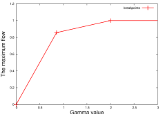
Figure 11. The value of the maximum flow, or equivalently the value of the minimum cut, as a function of $\gamma$ for the network in Figure 10.

In the following lemma we show that if there is any valid $\gamma$, then at least one breakpoint is valid.

Lemma 14.

Assume $\gamma^{*}\in(\gamma_{1},\gamma_{2})$ where $\gamma_{1},\gamma_{2}$ are two subsequent breakpoints of $\kappa(\gamma)$, or $\gamma_{1}=0$ and $\gamma_{2}$ is the first breakpoint, or $\gamma_{1}$ is the last breakpoint and $\gamma_{2}=\infty$. Assume $\gamma^{*}$ is valid for $\mathcal{N}(\gamma^{*})$, then, $\gamma$ is valid for $\mathcal{N}(\gamma)$ for all $\gamma\in[\gamma_{1},\gamma_{2}]$.

Proof 5.2.

Consider the network $\mathcal{N}(\gamma^{*})$. Assume that the maximum flow $f_{\gamma^{*}}$ is a valid maximum flow for $\mathcal{N}(\gamma^{*})$.

Assume first $\gamma^{\prime}\in(\gamma^{*},\gamma_{2}]$. We use the augmenting path algorithm [1] to obtain a maximum flow $f^{*}$ in the residual network $\mathcal{N}_{f_{\gamma^{*}}}(\gamma^{\prime})$, requiring that the augmenting path contains no cycles, which is a harmless restriction. Then, $f_{\gamma^{\prime}}:=f_{\gamma^{*}}+f^{*}$ is a maximum flow in $\mathcal{N}(\gamma^{\prime})$. Since $f_{\gamma^{*}}$ saturates edges from ${\mathord{\nnearrow}}$ to $MU_{1}$, $f_{\gamma^{\prime}}$ saturates edges from ${\mathord{\nnearrow}}$ to $MU_{1}$ as well , as flow along an augmenting path without cycles does not un-saturate edges to $MU_{1}$. We choose the minimum cut $(X,X^{\prime})$ for $\mathcal{N}(\gamma^{*})$ with respect to $f_{\gamma^{*}}$ such that $\overline{MU_{2}}\cap X^{\prime}=\emptyset$, or equivalently $\overline{MU_{2}}\subseteq X$. This is possible since $f_{\gamma^{*}}$ saturates all edges $(\overline{u}_{2},{\mathord{\ssearrow}})$ with $u_{2}\in MU_{2}$. The minimum cut for $f_{\gamma^{\prime}}$, then, can also be chosen as $(X,X^{\prime})$, as $(\gamma^{\prime},\kappa(\gamma^{\prime}))$ lies on the same line segment as $(\gamma^{*},\kappa(\gamma^{*}))$. Hence, $f_{\gamma^{\prime}}$ saturates the edges from $\overline{MU_{2}}$ to ${\mathord{\ssearrow}}$, which indicates that $f_{\gamma^{\prime}}$ is valid for $\mathcal{N}(\gamma^{\prime})$. Therefore, $\gamma^{\prime}$ is valid for $\mathcal{N}(\gamma^{\prime})$ for $\gamma^{\prime}\in(\gamma^{*},\gamma_{2}]$.

Now let $\gamma^{\prime}\in[\gamma_{1},\gamma^{*})$. For the valid maximum flow $f_{\gamma^{*}}$ we select the minimal cut $(X,X^{\prime})$ for $\mathcal{N}(\gamma^{*})$ such that $MU_{1}\cap X=\emptyset$. Let $d$ denote a valid distance function corresponding to $f_{\gamma^{*}}$. We replace $f_{\gamma^{*}}(\overline{v},{\mathord{\ssearrow}})$ by $\min\{f_{\gamma^{*}}(\overline{v},{\mathord{\ssearrow}}),c_{\gamma^{\prime}}(\overline{v},{\mathord{\ssearrow}})\}$ where $c_{\gamma^{\prime}}$ is the capacity function of $\mathcal{N}(\gamma^{\prime})$. The modified flow is a preflow for the network $\mathcal{N}(\gamma^{\prime})$. Moreover, $d$ stays a valid distance function as no new residual edges are introduced. Then, we apply the preflow algorithm to get a maximum flow $f_{\gamma^{\prime}}$ for the network $\mathcal{N}(\gamma^{\prime})$. Since no flow is pushed back from the sink, edges from $\overline{MU_{2}}$ to ${\mathord{\ssearrow}}$ are kept saturated. Since $(\gamma^{*},\kappa(\gamma^{*}))$ and $(\gamma^{\prime},\kappa(\gamma^{\prime}))$ are on the same line segment, the minimal cut for $f_{\gamma^{\prime}}$ can also be chosen as $(X,X^{\prime})$, which indicates that $f_{\gamma^{\prime}}$ saturates all edges to $MU_{1}$. This implies that $\gamma^{\prime}$ is valid for $\mathcal{N}(\gamma^{\prime})$ for $\gamma^{\prime}\in[\gamma_{1},\gamma^{*})$.

In Example 5.1.2, only one breakpoint is valid. In the following example we show that it is in general possible that more than one breakpoint is valid.

Figure 12. A network in which more than one breakpoint is valid.

Consider the network depicted in Figure 12. By a similar analysis as Example 5.1.2, we can compute that there are three breakpoints $\frac{1}{2}$, $1$ and $2$. Assuming that $MU_{1}=\{o_{1}\}$ and $MU_{2}=\{o_{2}\}$, we show that all $\gamma\in[\frac{1}{2},1]$ are valid. We send $\frac{\gamma}{4}$ amount of flow along the path ${\mathord{\nnearrow}},o_{1},\overline{o_{2}},{\mathord{\ssearrow}}$, and $\frac{1}{4}-\frac{\gamma}{4}$ amount of flow along the path ${\mathord{\nnearrow}},o_{1},\overline{v_{2}},{\mathord{\ssearrow}}$. If $\gamma\in[\frac{1}{2},1]$, then $0\leq\frac{1}{4}-\frac{\gamma}{4}\leq\frac{\gamma}{4}$ implying that the flow on edge $(\overline{v_{2}},{\mathord{\ssearrow}})$ satisfies the capacity constraints. Obviously this flow is feasible, and all $\gamma\in[\frac{1}{2},1]$ are valid for $\mathcal{N}(\gamma)$.

As we would expect now, it is sufficient to consider only the breakpoints of $\mathcal{N}(\gamma)$:

Lemma 15.

There exists a valid $\gamma$ for $\mathcal{N}(\gamma)$ iff one of the breakpoints of $\mathcal{N}(\gamma)$ is valid.

Proof 5.3.

If there exists a valid $\gamma$ for $\mathcal{N}(\gamma)$, Lemma 14 guarantees that one of the breakpoints of $\kappa(\gamma)$ is valid. The other direction is trivial.

For a given breakpoint, we need to solve one feasible flow problem to check whether it is valid. In the network $\mathcal{N}(\gamma)$ the capacities of the edges leading to the sink are increasing functions of a real-valued parameter $\gamma$. If we reverse $\mathcal{N}(\gamma)$, we get a parametric network that satisfies the conditions in [18]: The capacities emanating from ${\mathord{\nnearrow}}$ are non-decreasing functions of $\gamma$. So we can apply the breakpoint algorithm [18] to obtain all of the breakpoints of $\mathcal{N}(\gamma)$.

5.1.3. The Algorithm for DTMCs

Let $\mathcal{M}$ be a DTMC and let $\textnormal{SimRel}_{w}(\mathcal{M})$ denote the weak simulation algorithm, which is obtained by replacing line 6 of $\textnormal{SimRel}_{s}(\mathcal{M})$ in Algorithm 1 by: if $s_{1}\precapprox_{R}s_{2}$. The condition $s_{1}\precapprox_{R}s_{2}$ is checked in $\textnormal{Ws}(\mathcal{M},s_{1},s_{2},R)$, shown as Algorithm 8.

Algorithm 8: Algorithm to check whether $s_{1}\precapprox_{R}s_{2}$.

$\textnormal{Ws}(\mathcal{M},s_{1},s_{2},R)$

8.1:  if $\mathit{post}(s_{1})\subseteq R^{-1}(s_{2})$ then

8.2:        return $\mathbf{true}$

8.3:  if $\mathit{post}(s_{2})\subseteq R(s_{1})$ then

8.4:        $U_{1}\leftarrow\{s_{1}^{\prime}\in\mathit{post}(s_{1})\mid s_{1}^{\prime}\not\in R^{-1}(s_{2})\}$

8.5:        return ($\forall u_{1}\in U_{1}.\ \exists s\in\mathit{post}(reach(s_{2})\cap R(s_{1})).\ s\in R(u_{1})$)

8.6:  Compute all of the breakpoints $b_{1}<b_{2}<\ldots<b_{j}$ of $\mathcal{N}(\gamma)$

8.7:  return ($\exists i\in\{1,\ldots,j\}.\ b_{i}\mbox{ is valid for }\mathcal{N}(b_{i})$)

The first part of the algorithm is the preprocessing part. Line 1 tests for the case that $s_{1}$ could perform only stutter steps with respect to the current relation $R$. If line 5 is reached, $s_{1}$ has at least one visible step, and all successors of $s_{2}$ can simulate $s_{1}$ up to the current relation $R$. In this case we need to check the reachability Condition 3 of Definition 2.2.3, which is performed in line 5. Recall that $reach(s)$ denotes the set of states that are reachable from $s$ with positive probability. If the algorithm does not terminate in the preprocessing part, the breakpoints of the network $\mathcal{N}(\gamma)$ are computed. Then, corresponding to Lemma 15, we check whether one of the breakpoints is valid. We show the correctness of the algorithm Ws:

Lemma 16.

The algorithm $\textnormal{Ws}(\mathcal{M},s_{1},s_{2},R)$ returns true iff $s_{1}\precapprox_{R}s_{2}$.

Proof 5.4.

We first show the only if direction. Assume that $\textnormal{Ws}(\mathcal{M},s_{1},s_{2},R)$ returns true. We consider three possible cases:

1. The algorithm returns true at line 2. For this case we have that $\mathit{post}(s_{1})\subseteq R^{-1}(s_{2})$. We choose $U_{1}=\emptyset,V_{1}=\mathit{post}(s_{1})$, $U_{2}=\mathit{post}(s_{2})$ and $V_{2}=\emptyset$ to fulfill the conditions in Definition 2.2.3. Hence, $s_{1}\precapprox_{R}s_{2}$.

2. The algorithm returns true at line 5. If the algorithm reaches line 5, the following conditions hold: there exists a state $s_{1}^{\prime}\in\mathit{post}(s_{1})$ such that $s_{1}^{\prime}\not\in R^{-1}(s_{2})$ (line 1), and $\mathit{post}(s_{2})\subseteq R(s_{1})$ (line 3). Let $U_{1}=\{s_{1}^{\prime}\in\mathit{post}(s_{1})\mid s_{1}^{\prime}\not\in R^{-1}(s_{2})\}$, and define $\delta_{i}$ by: $\delta_{1}(s)=1$ if $s\in U_{1}$, and $0$ otherwise, $\delta_{2}(s)=0$ for all $s\in S$. By construction, to show $s_{1}\precapprox_{R}s_{2}$ we only need to show the reachability condition. Since the algorithm returns true at line 5, it holds that for each $u_{1}\in U_{1}$, there exists $s\in\mathit{post}(reach(s_{2})\cap R(s_{1}))$ such that $s\in R(u_{1})$. This is exactly the reachability condition required by weak simulation up to $R$, thus $s_{1}\precapprox_{R}s_{2}$.

3. The algorithm returns true at line 7. Thus, there exists breakpoint $b_{i}$ which is valid for $\mathcal{N}(b_{i})$. Then, there exists a state $s_{1}^{\prime}\in\mathit{post}(s_{1})$ such that $s_{1}^{\prime}\not\in R^{-1}(s_{2})$, and $s_{2}^{\prime}\in\mathit{post}(s_{2})$ such that $s_{2}^{\prime}\not\in R(s_{1})$. By Lemma 13, we have that $s_{1}\precapprox_{R}s_{2}$.

Now we show the if direction. Assume that Ws returns false. It is sufficient to show that $s_{1}\not\precapprox_{R}s_{2}$. We consider two cases:

1. The algorithm returns false at line 5. This implies that there exists a state $s_{1}^{\prime}\in\mathit{post}(s_{1})$ such that $s_{1}^{\prime}\not\in R^{-1}(s_{2})$ (line 1), and $\mathit{post}(s_{2})\subseteq R(s_{1})$ (line 3). All states $s_{1}^{\prime}\in\mathit{post}(s_{1})$ with $s_{1}^{\prime}\not\in R^{-1}(s_{2})$ must be put into $U_{1}$. However, since the algorithm returns false at line 5, it holds that there exists a state $u_{1}\in U_{1}$, such that there does not exist $s\in\mathit{post}(reach(s_{2})\cap R(s_{1}))$ with $s\in R(u_{1})$. Thus the reachability condition of Definition 2.2.3 is violated which implies that $s_{1}\not\precapprox_{R}s_{2}$.

2. The algorithm returns false at line 7. Then, there exists a state $s_{1}^{\prime}\in\mathit{post}(s_{1})$ such that $s_{1}^{\prime}\not\in R^{-1}(s_{2})$, and $s_{2}^{\prime}\in\mathit{post}(s_{2})$ such that $s_{2}^{\prime}\not\in R(s_{1})$. Moreover, for all breakpoints $b$ of $\mathcal{N}(\gamma)$, $b$ is not valid for $\mathcal{N}(b)$. By Lemma 15, there does not exist a valid $\gamma$ for $\mathcal{N}(\gamma)$. By Lemma 13, we have that $s_{1}\not\precapprox_{R}s_{2}$.∎

Now we state the correctness of the algorithm $\textnormal{SimRel}_{w}$ for DTMCs:

Theorem 17.

If $\textnormal{SimRel}_{w}(\mathcal{M})$ terminates, the returned relation $R$ equals $\precapprox_{\mathcal{M}}$.

Proof 5.5.

The proof follows exactly the lines of the proof of Theorem 2. Let iteration $k$ be the last iteration of Ws. Then, by Lemma 16, for each pair $(s_{1},s_{2})\in R_{k}$, it holds that $s_{2}$ weakly simulates $s_{1}$ up to $R_{k}$, so $R_{k}$ is a weak simulation. On the other hand, one can prove by induction that each $R_{i}$ is coarser than $\precapprox$.

Complexity.

For $(s_{1},s_{2})\in R$, we have shown that to check whether $s_{1}\precapprox_{R}s_{2}$ we could first compute the breakpoints of $\mathcal{N}(\gamma)$, then solve $\mathcal{O}(\left\lvert V\right\rvert)$ many maximum flow problems. To achieve a better bound, we first prove that applying a binary search method over the breakpoints, we only need to consider $\mathcal{O}(\log\left\lvert V\right\rvert)$ breakpoints, and thus solve $\mathcal{O}(\log\left\lvert V\right\rvert)$ maximum flow problems.

Assume that the sets $MU_{i}$ and $PV_{i}$ for $i=1,2$ are constructed as before for $\mathcal{N}(\gamma)$. Recall that a flow function $f$ of $\mathcal{N}(\gamma)$ is valid for $\mathcal{N}(\gamma)$ iff $f$ saturates all edges $({\mathord{\nnearrow}},u_{1})$ with $u_{1}\in MU_{1}$ and all edges $(\overline{u_{2}},{\mathord{\ssearrow}})$ with $u_{2}\in MU_{2}$. If $f$ is also a maximum flow, we say that $f$ is a valid maximum flow of $\mathcal{N}(\gamma)$. We first reformulate Lemma 13 using maximum flow.

Lemma 18.

There exists a valid flow $f$ for $\mathcal{N}(\gamma)$ iff there exists a valid maximum flow $f_{m}$ for $\mathcal{N}(\gamma)$.

Proof 5.6.

Assume there exists a valid flow $f$ for $\mathcal{N}(\gamma)$. We let $\mathcal{N}_{f}(\gamma)$ denote the residual network. We use the augmenting path algorithm to get a maximum flow $f^{\prime}$ in the residual network $\mathcal{N}_{f}(\gamma)$. Assume that the augmenting path contains no cycles, which is a harmless restriction. Let $f_{m}=f+f^{\prime}$. Obviously, $f_{m}$ is a maximum flow for $\mathcal{N}(\gamma)$, and it saturates all of the edges saturated by $f$. Hence, $f_{m}$ is valid for $\mathcal{N}(\gamma)$. The other direction is simple, since a valid maximum flow is also a valid flow for $\mathcal{N}(\gamma)$.

$s_{1}$$u_{1}$ $\frac{1}{2}$ $v_{1}$ $\frac{1}{2}$   $s_{1}$$u_{2}$ $\frac{1}{2}$ $v_{2}$ $\frac{1}{2}$          

Figure 13. A simple DTMC for illustrating that not all maximum flows are valid.

We first discuss how to get a valid maximum flow provided that $\gamma$ is valid. Observe that even if $\gamma$ is valid for $\mathcal{N}(\gamma)$, not all maximum flows for $\mathcal{N}(\gamma)$ are necessarily valid. Consider the DTMC on the left part of Figure 13. Assume that the relation $R$ is given by $\{(s_{1},s_{2}),$ $(s_{1},v_{2}),$ $(v_{1},s_{2}),$ $(u_{1},u_{2}),$ $(u_{1},v_{2})\}$ and consider the pair $(s_{1},s_{2})$. Thus, we have that $PV_{1}=\{v_{1}\},MU_{1}=\{u_{1}\},PV_{2}=\{v_{2}\},MU_{2}=\{u_{2}\}$. The network $\mathcal{N}(\gamma)$ is depicted on the right part of Figure 13. The maximum flow $f$ for $\mathcal{N}(1)$ has value $0.5$. If $f$ contains positive sub-flow along the path ${\mathord{\nnearrow}},u_{1},\overline{v_{2}},{\mathord{\ssearrow}}$, it does not saturate the edge $(\overline{u_{2}},{\mathord{\ssearrow}})$. On the contrary, the flow along the single path ${\mathord{\nnearrow}},u_{1},\overline{u_{2}},{\mathord{\ssearrow}}$ with value $0.5$ would be a valid maximum flow. This example gives us the intuition to use the augmenting path through edges between $MU_{1}$ and $\overline{MU_{2}}$ as much as possible. For this purpose we define a cost function $\mathit{cost}$ from edges in $\mathcal{N}(\gamma)$ to real numbers as follows: $\mathit{cost}(u_{1},\overline{u_{2}})=2$ for $u_{1}\in MU_{1}$ and $u_{2}\in MU_{2}$, $\mathit{cost}(u_{1},\overline{v_{2}})=1$ for $u_{1}\in MU_{1}$ and $v_{2}\in PV_{2}$, $\mathit{cost}(v_{1},\overline{u_{2}})=1$ for $v_{1}\in PV_{1}$ and $u_{2}\in MU_{2}$, $\mathit{cost}(s,s^{\prime})=0$ otherwise. The costs of edges starting from source, or ending at sink, or in $PV_{1}\times\overline{PV_{2}}$ are $0$. The cost of a flow $f$ is defined by $\mathit{cost}(f)=\sum_{e\in E}f(e)\mathit{cost}(e)$. By definition of the cost function, we have the property $\mathit{cost}(f)=f({\mathord{\nnearrow}},MU_{1})+f(\overline{MU_{2}},{\mathord{\ssearrow}})$, i.e., the cost equals the sum of the amount of flow from ${\mathord{\nnearrow}}$ into $MU_{1}$ and from $\overline{MU_{2}}$ into ${\mathord{\ssearrow}}$.

Lemma 19.

Assume that $\gamma>0$ is valid for $\mathcal{N}(\gamma)$. Let $f_{\gamma}$ denote a maximum flow over $\mathcal{N}(\gamma)$ with maximum cost. Then, $f_{\gamma}$ is valid for $\mathcal{N}(\gamma)$.

Proof 5.7.

By Lemma 18, provided $\gamma$ is valid for $\mathcal{N}(\gamma)$, there exists a valid maximum flow function $g$ for $\mathcal{N}(\gamma)$. Since $g$ saturates edges to $MU_{1}$ and from $MU_{2}$, obviously, $\mathit{cost}(g)=\mathbf{P}(s_{1},MU_{1})+\gamma\mathbf{P}(s_{2},MU_{2})$. Assume that $f_{\gamma}$ is not valid, which indicates that $f_{\gamma}$ does not saturate an edge $({\mathord{\nnearrow}},u_{1})$ with $u_{1}\in MU_{1}$ or an edge $(\overline{u_{2}},{\mathord{\ssearrow}})$ with $u_{2}\in\overline{MU_{2}}$. Then, $\mathit{cost}(f_{\gamma})=f({\mathord{\nnearrow}},MU_{1})+f(\overline{MU_{2}},{\mathord{\ssearrow}})<\mathbf{P}(s_{1},MU_{1})+\gamma\mathbf{P}(s_{2},MU_{2})=\mathit{cost}(g)$. This contradicts the assumption that $f_{\gamma}$ has maximum cost.

Let $\mathcal{N}_{U}(\gamma)$ denote the subnetwork of $\mathcal{N}(\gamma)$ where the set of vertices is restricted to $MU_{1},\overline{MU_{2}}$ and $\{{\mathord{\nnearrow}},{\mathord{\ssearrow}}\}$. The following lemma discusses how to construct a maximum flow with maximum cost.

Lemma 20.

Assume that $f^{*}$ is an arbitrary maximum flow of $\mathcal{N}_{U}(\gamma)$ and $\tilde{f}$ is an arbitrary maximum flow in the residual network $\mathcal{N}_{f^{*}}(\gamma)$ with the residual edges from $MU_{1}$ back to ${\mathord{\nnearrow}}$ removed, as well as the residual edges from ${\mathord{\ssearrow}}$ back to $\overline{MU_{2}}$. Then $f_{\gamma}=f^{*}+\tilde{f}$ is a maximum flow over $\mathcal{N}(\gamma)$ with maximum cost.

Proof 5.8.

Recall that the cost of $f_{\gamma}$ is equal to $\mathit{cost}(f_{\gamma})=f_{\gamma}({\mathord{\nnearrow}},MU_{1})+f_{\gamma}(\overline{MU_{2}},{\mathord{\ssearrow}})$. Assume that $\mathit{cost}(f_{\gamma})$ is not maximal for the sake of contradiction. Let $f$ be a maximum flow such that $\mathit{cost}(f_{\gamma})<\mathit{cost}(f)$. Without loss of generality, we assume that $f_{\gamma}({\mathord{\nnearrow}},MU_{1})<f({\mathord{\nnearrow}},MU_{1})$. It holds that $f_{\gamma}=f^{*}+\tilde{f}$ where $f^{*}$ is a maximum flow of $\mathcal{N}_{U}(\gamma)$, and $\tilde{f}$ is a maximum flow in the residual network $\mathcal{N}_{f^{*}}(\gamma)$ with the residual edges from $MU_{1}$ back to ${\mathord{\nnearrow}}$ removed, as well as the residual edges from ${\mathord{\ssearrow}}$ back to $\overline{MU_{2}}$. On the one hand, $f^{*}$ sends as much flow as possible along $MU_{1}$ in $\mathcal{N}_{U}(\gamma)$. Since in the residual network $\mathcal{N}_{f^{*}}(\gamma)$ edges from $MU_{1}$ back to ${\mathord{\nnearrow}}$ are removed, this guarantees that no flow can be sent back to ${\mathord{\nnearrow}}$ from $MU_{1}$. On the other hand, $\tilde{f}$ sends as much flow as possible from $MU_{1}$ to $\overline{PV_{2}}$ (and also from $PV_{1}$ to $\overline{MU_{2}}$) in $\mathcal{N}_{f^{*}}(\gamma)$. Thus, $f_{\gamma}({\mathord{\nnearrow}},MU_{1})$ must be maximal which contradicts the assumption $f_{\gamma}({\mathord{\nnearrow}},MU_{1})<f({\mathord{\nnearrow}},MU_{1})$.

Assume that $\gamma^{*}$ is not valid. The following lemma determines, provided a valid $\gamma$ exists, whether it is greater or smaller than $\gamma^{*}$:

Lemma 21.

Let $\gamma^{*}\in[0,\infty)$, and let $f$ be a maximum flow function with maximum cost for $\mathcal{N}(\gamma^{*})$, as described in Lemma 20. Then,

1. If $f$ saturates all edges $({\mathord{\nnearrow}},u_{1})$ with $u_{1}\in MU_{1}$ and $(\overline{u_{2}},{\mathord{\ssearrow}})$ with $u_{2}\in MU_{2}$, $\gamma^{*}$ is valid for $\mathcal{N}(\gamma^{*})$.

2. Assume that $\exists u_{1}\in MU_{1}$ such that $({\mathord{\nnearrow}},u_{1})$ is not saturated by $f$, and all edges $(\overline{u_{2}},{\mathord{\ssearrow}})$ with $u_{2}\in MU_{2}$ are saturated by $f$. Then, $\gamma^{*}$ is not valid. If there exists a valid $\gamma$, $\gamma>\gamma^{*}$.

3. Assume that all edges $({\mathord{\nnearrow}},u_{1})$ with $u_{1}\in MU_{1}$ are saturated by $f$, and $\exists u_{2}\in MU_{2}$ such that $(\overline{u_{2}},{\mathord{\ssearrow}})$ is not saturated by $f$. Then, $\gamma^{*}$ is not valid. If there exists a valid $\gamma$, $\gamma<\gamma^{*}$.

4. Assume that $\exists u_{1}\in MU_{1}$ and $\exists u_{2}\in MU_{2}$ such that $({\mathord{\nnearrow}},u_{1})$ and $(\overline{u_{2}},{\mathord{\ssearrow}})$ are not saturated by $f$. Then, there does not exist a valid $\gamma$.

Proof 5.9.

$1:$ Follows directly from the definition. $2:$ In this case, $f({\mathord{\nnearrow}},u_{1})<\mathbf{P}(s_{1},u_{1})$ for some $u_{1}\in MU_{1}$. To saturate $({\mathord{\nnearrow}},u_{1})$, without un-saturating other edges from ${\mathord{\nnearrow}}$ to $MU_{1}$, we have to increase the capacities of edges leading to ${\mathord{\ssearrow}}$, thus increase $\gamma^{*}$. $3:$ Similar to the previous case. $4:$ Combining $2$ and $3$.

According to the above lemma, we can use the binary search method over the breakpoints to check whether there exists a valid breakpoint for $\mathcal{N}(\gamma)$. Since there are at most $\mathcal{O}(\left\lvert V\right\rvert)$ breakpoints, we invoke the maximum flow algorithm at most $\mathcal{O}(\log\left\lvert V\right\rvert)$ times where $\left\lvert V\right\rvert$ is the number of vertices of $\mathcal{N}(\gamma)$.

Theorem 22.

The algorithm $\textnormal{SimRel}_{w}(\mathcal{M})$ runs in time $\mathcal{O}(m^{2}n^{3})$ and in space $\mathcal{O}(n^{2})$. If the fanout $g$ is bounded by a constant, the time complexity is $\mathcal{O}(n^{5})$.

Proof 5.10.

First, we consider a pair $(s_{1},s_{2})$ out of the current relation $R_{i}$. Look at a single call of $\textnormal{Ws}(\mathcal{M},s_{1},s_{2},R_{i})$. By saving the current relation sets $R$ and $R^{-1}$ in a two dimensional array, the conditions $s\in R(s^{\prime})$ or $s\in R^{-1}(s^{\prime})$ can be checked in constant time. Hence, line 1 takes time $\left\lvert\mathit{post}(s_{1})\right\rvert$. To construct the set $reach(s)$ for a state $s$, BFS can be used, which has complexity $\mathcal{O}(m)$. The size of the set $reach(s)$ is bounded by $n$. Therefore, we need $\mathcal{O}(\left\lvert\mathit{post}(s_{1})\right\rvert n)$ time at lines 3–5.

The algorithm computes all breakpoints of the network $\mathcal{N}(\gamma)$ (with respect to $s_{1},s_{2}$ and $R$) using the breakpoint algorithm [18, p. 37–42]. Assume the set of vertices of $\mathcal{N}(\gamma)$ is partitioned into subsets $V_{1}$ and $V_{2}$ similar to the network described in Section 4.1. The number of edges of the network is at most $\left\lvert E\right\rvert:=\left\lvert V_{1}\right\rvert\left\lvert V_{2}\right\rvert-1$. Let $\left\lvert V\right\rvert:=\left\lvert V_{1}\right\rvert+\left\lvert V_{2}\right\rvert$, and, without loss of generality, we assume that $\left\lvert V_{1}\right\rvert\leq\left\lvert V_{2}\right\rvert$. For our bipartite networks, the time complexity [18, p. 42] for computing the breakpoints is $\mathcal{O}(\left\lvert V_{1}\right\rvert\left\lvert E\right\rvert\log(\frac{\left\lvert V_{1}\right\rvert^{2}}{\left\lvert E\right\rvert}+2))$ which can be simplified to $\mathcal{O}(\left\lvert V_{1}\right\rvert^{2}\left\lvert V_{2}\right\rvert)$. Then, the binary search can be applied over all of the breakpoints to check whether at least one breakpoint is valid, for which we need to solve at most $\mathcal{O}(\log\left\lvert V\right\rvert)$ many maximum flow problems. For our network $\mathcal{N}(\gamma)$, the best known complexity of the maximum flow problem is $\mathcal{O}(\left\lvert V\right\rvert^{3}/\log\left\lvert V\right\rvert)$ [14]. As indicated in the proof of Lemma 4, the distance function is bounded by $4\left\lvert V_{1}\right\rvert$ for our bipartite network. Applying this fact in the complexity analysis in [14], we get the corresponding complexity for computing maximum flow for bipartite networks $\mathcal{O}(\left\lvert V_{1}\right\rvert\left\lvert V\right\rvert^{2}/\log\left\lvert V\right\rvert)$. Hence, the complexity for the $\mathcal{O}(\log|V|)$-invocations of the maximum flow algorithm is bounded by $\mathcal{O}(\left\lvert V_{1}\right\rvert\left\lvert V\right\rvert^{2})$. As $\left\lvert V\right\rvert\leq 2\left\lvert V_{2}\right\rvert$, the complexity is equal to $\mathcal{O}(\left\lvert V_{1}\right\rvert\left\lvert V_{2}\right\rvert^{2})$. Summing over all $(s_{1},s_{2})$ over all $R_{i}$, we get the overall complexity of $\textnormal{SimRel}_{w}(\mathcal{M})$:

$$\sum_{i=1}^{k}\sum_{(s_{1},s_{2})\in R_{i}}(\left\lvert\mathit{post}(s_{1})\right\rvert+m+\left\lvert\mathit{post}(s_{1})\right\rvert n+\left\lvert V_{1}\right\rvert\left\lvert V_{2}\right\rvert^{2})\leq 4knm^{2}$$ (13)

Recall that in the algorithm $\textnormal{SimRel}_{w}(\mathcal{M})$, the number of iterations $k$ is at most $n^{2}$. Hence, the time complexity amounts to $\mathcal{O}(m^{2}n^{3})$. The space complexity is $\mathcal{O}(n^{2})$ because of the representation of $R$. If the fanout is bounded by a constant $g$, we have $m\leq gn$, and get the complexity $\mathcal{O}(n^{5})$.

5.1.4. An Improvement

The algorithm $\textnormal{Ws}(\mathcal{M},s_{1},s_{2},R)$ is dominated by the part in which all breakpoints ($\mathcal{O}(n)$ many) must be computed, and a binary search is applied to the breakpoints, with $\mathcal{O}(\log n)$ many feasible flow problems. In this section we discuss how to achieve an improved algorithm if the network $\mathcal{N}(\gamma)$ can be partitioned into sub-networks.

Let $H$ denote the sub-relation $R\cap[(\mathit{post}(s_{1})\cup\{s_{1}\})\times(\mathit{post}(s_{2})\cup\{s_{2}\})]$, which is the local fragment of the relation $R$. Now let $A_{1},A_{2},\ldots A_{\mathit{h}}$ enumerate the classes of the equivalence relation $(H\cup H^{-1})^{*}$ generated by $H$, where $\mathit{h}$ denotes the number of classes. W. l. o. g., we assume in the following that $A_{\mathit{h}}$ is the equivalence class containing $s_{1}$ and $s_{2}$, i. e., $s_{1},s_{2}\in A_{\mathit{h}}$. The following lemma gives some properties of the sets $A_{i}$ provided that $s_{1}\precapprox_{R}s_{2}$:

Lemma 23.

For $(s_{1},s_{2})\in R$, assume that there exists a state $s_{1}^{\prime}\in\mathit{post}(s_{1})$ such that $s_{1}^{\prime}\not\in R^{-1}(s_{2})$, and $s_{2}^{\prime}\in\mathit{post}(s_{2})$ such that $s_{2}^{\prime}\not\in R(s_{1})$. Let $A_{1},\ldots,A_{\mathit{h}}$ be the sets constructed for $(s_{1},s_{2})$ as above. If $s_{1}\precapprox_{R}s_{2}$, the following hold:

1. $\mathbf{P}(s_{1},A_{i})>0$ and $\mathbf{P}(s_{2},A_{i})>0$ for all $i<\mathit{h}$,

2. $\gamma_{i}={K_{1}}/{K_{2}}$ for all $i<\mathit{h}$ where $\gamma_{i}={\mathbf{P}(s_{1},A_{i})}/{\mathbf{P}(s_{2},A_{i})}$

Proof 5.11.

Since $s_{1}\precapprox_{R}s_{2}$, we let $\delta_{i},U_{i},V_{i},\Delta$ (for $I=1,2$) as described in Definition 2.2.3. Because of states $s_{1}^{\prime}$ and $s_{2}^{\prime}$, we have $K_{1}>0,K_{2}>0$. Let $\mathit{post}_{i}(s_{j})=A_{i}\cap\mathit{post}(s_{j})$ for $i=1,\ldots,\mathit{h}$ and $j=1,2$. We prove the first part. For $i<\mathit{h}$, the set $A_{i}$ does not contain $s_{1}$ nor $s_{2}$, but only (some of) their successors, so it is impossible that both $\mathbf{P}(s_{1},A_{i})=0$ and $\mathbf{P}(s_{2},A_{i})=0$. W. l. o. g., assume that $\mathbf{P}(s_{1},A_{i})>0$. There exists $t\in\mathit{post}_{i}(s_{1})$ such that $\mathbf{P}(s_{1},t)>0$. Obviously $\delta_{1}(t)=1$, thus: $0<\mathbf{P}(s_{1},t)=(K_{1}\Delta(t,U_{2}))/\delta_{1}(t)=K_{1}\Delta(t,U_{2})$ which implies that $\exists u_{2}\in A_{i}$ with $\Delta(t,u_{2})>0$. Hence, $\mathbf{P}(s_{2},u_{2})=K_{2}\Delta(U_{1},u_{2})\geq K_{2}\Delta(t,u_{2})>0.$ Now we prove the second part. It holds that:

$$\mathbf{P}(s_{1},A_{i})=\sum_{a_{i}\in A_{i}}\mathbf{P}(s_{1},a_{i})=\sum_{a_{i}\in\mathit{post}_{i}(s_{1})}\mathbf{P}(s_{1},a_{i})\stackrel{{\scriptstyle(*)}}{{=}}\sum_{a_{i}\in\mathit{post}_{i}(s_{1})}\frac{K_{1}\Delta(a_{i},U_{2})}{\delta_{1}(a_{i})}\\ \stackrel{{\scriptstyle(!)}}{{=}}K_{1}\cdot\sum_{a_{i}\in\mathit{post}_{i}(s_{1})}\Delta(a_{i},U_{2})\stackrel{{\scriptstyle({\dagger})}}{{=}}K_{1}\cdot\sum_{a_{i}\in\mathit{post}_{i}(s_{1})}\Delta(a_{i},A_{i})=K_{1}\cdot\sum_{a_{i}\in A_{i}}\Delta(a_{i},A_{i})$$

where $(*)$ follows from Condition 2b of Definition 2.2.3, $(!)$ follows from the equation $\delta_{1}(a_{i})=1$ for all $a_{i}\in\mathit{post}_{i}(a_{1})$ with $i<n$, and $({\dagger})$ follows from the fact that if $a\in\mathit{post}_{i}(s_{1})$, then $\Delta(a,b)=0$ for $b\in U_{2}\backslash\mathit{post}_{i}(s_{2})$. In the same way, we get $\mathbf{P}(s_{2},A_{i})=K_{2}\cdot\sum_{a_{i}\in A_{i}}\Delta(A_{i},a_{i})$. Therefore, $\gamma_{i}={K_{1}}/{K_{2}}$ for $1\leq i<\mathit{h}$.

Algorithm 9: Algorithm to check whether $s_{1}\precapprox_{R}s_{2}$ tailored to DTMCs.

$\textnormal{WsImproved}(\mathcal{M},s_{1},s_{2},R)$

9.1:  Construct the partition $A_{1},\ldots,A_{\mathit{h}}$ (* Assume that $h>1$ *)

9.2:  for all $i\leftarrow 1,2,\ldots\mathit{h}-1$ do

9.3:        if $\mathbf{P}(s_{1},A_{i})=\mathbf{P}(s_{2},A_{i})=0$ then

9.4:              raise error

9.5:        else if $\mathbf{P}(s_{1},A_{i})=0$ or $\mathbf{P}(s_{2},A_{i})=0$ then

9.6:              return $\mathbf{false}$

9.7:        else

9.8:              $\gamma_{i}\leftarrow\frac{\mathbf{P}(s_{1},A_{i})}{\mathbf{P}(s_{2},A_{i})}$

9.9:  if $\gamma_{i}\not=\gamma_{j}$ for some $i,j<\mathit{h}$ then

9.10:        return $\mathbf{false}$

9.11:  return ($\gamma_{1}$ is valid for $\mathcal{N}(\gamma_{1})$)

For the case $\mathit{h}>1$, the above lemma allows to check whether $s_{1}\precapprox_{R}s_{2}$ efficiently. For this case we replace lines 6–7 of Ws by the sub-algorithm WsImproved in Algorithm 9. The partition $A_{1},\ldots,A_{\mathit{h}}$ is constructed in line 1. Lines 2–10 follow directly from Lemma 23: if $\gamma_{i}\neq\gamma_{j}$ for some $i,j<h$, we conclude from Lemma 23 that $s_{1}\not\precapprox_{R}s_{2}$. Line 11 follows from the following lemma, which is the counterpart of Lemma 13:

Lemma 24.

For $(s_{1},s_{2})\in R$, assume that there exists a state $s_{1}^{\prime}\in\mathit{post}(s_{1})$ such that $s_{1}^{\prime}\not\in R^{-1}(s_{2})$, and $s_{2}^{\prime}\in\mathit{post}(s_{2})$ such that $s_{2}^{\prime}\not\in R(s_{1})$. Assume that $\mathit{h}>1$, and assume $\textnormal{WsImproved}(\mathcal{M},s_{1},s_{2},R)$ reaches line 11. Then, $s_{1}\precapprox_{R}s_{2}$ iff $\gamma_{1}$ is valid for $\mathcal{N}(\gamma_{1})$.

Proof 5.12.

First, assume that $s_{1}\precapprox_{R}s_{2}$. According to Lemma 13, there exists a valid $\gamma^{*}$ for $\mathcal{N}(\gamma^{*})$. As in the proof of Lemma 13, $\gamma^{*}={K_{1}}/{K_{2}}$ is valid for $\mathcal{N}(\gamma^{*})$. If Ws reaches line 11, by Lemma 23, we have $\gamma_{1}={K_{1}}/{K_{2}}$, hence, $\gamma_{1}$ is valid for $\mathcal{N}(\gamma_{1})$. The other direction follows directly from Lemma 13.

Consider the DTMC in Figure 8 together with the relation $R=\{(s_{1},s_{2})$, $(s_{1},v_{2}),(v_{1},s_{2}),(u_{1},u_{2}),(o_{1},o_{2}),(o_{1},v_{2}),(v_{1},o_{3}),(v_{1},v_{2}),(o_{2},o_{1})\}$. We obtain the relation $H=R\backslash\{(o_{2},o_{1})\}$. We get two partitions $A_{1}=\{u_{1},u_{2}\}$ and $A_{2}=\{s_{1},s_{2},v_{1},v_{2},o_{1},o_{2},o_{3}\}$. In this case we have $\mathit{h}=2$. Recall that $MU_{1}=\{u_{1},o_{1}\}$, $MU_{2}=\{u_{2},o_{2},o_{3}\}$, $PV_{1}=\{v_{1}\}$, $PV_{2}=\{v_{2}\}$. We have $\mathbf{P}(s_{1},A_{1})=\frac{1}{4}$ and $\mathbf{P}(s_{2},A_{1})=\frac{1}{8}$. Hence, $\gamma_{1}={\mathbf{P}(s_{1},A_{1})}/{\mathbf{P}(s_{2},A_{1})}=2$. As we have shown in Example 5.1.1, $2$ is valid for the network $\mathcal{N}(2)$. Hence, $s_{1}\precapprox_{R}s_{2}$.

Assume that $(s_{1},s_{2})\in R_{1}$ such that $h>1$ in the first iteration of $\textnormal{SimRel}_{w}$. We consider the set $A_{1}$ and let $\gamma_{1}={\mathbf{P}(s_{1},A_{1})}/{\mathbf{P}(s_{2},A_{1})}$. If $A_{1}$ is not split in the next iteration, $\gamma_{1}$ would not change, and hence, we can reuse the network constructed in the last iteration. Assume that in the next iteration $A_{1}$ is split into two sets $A_{1}^{a}$ and $A_{1}^{b}$. There are two possibilities:

1. either ${\mathbf{P}(s_{1},A_{1}^{a})}/{\mathbf{P}(s_{2},A_{1}^{b})}={\mathbf{P}(s_{1},A_{1}^{a})}/{\mathbf{P}(s_{2},A_{1}^{b})}$. This implies that both of them are equal to $\gamma_{1}$. If all $A_{i}$ are split like $A_{1}$, we just check whether $\gamma_{1}$ is valid for $\mathcal{N}(\gamma_{1})$.

2. or ${\mathbf{P}(s_{1},A_{1}^{a})}/{\mathbf{P}(s_{2},A_{1}^{b})}\not={\mathbf{P}(s_{1},A_{1}^{a})}/{\mathbf{P}(s_{2},A_{1}^{b})}$. This case is simple, we conclude $s_{1}\not\precapprox_{R}s_{2}$ because of Lemma 23.

This indicates that once in the first iteration $\gamma_{1}$ is determined for $(s_{1},s_{2})$, either it does not change throughout the iterations, or we conclude that $s_{1}\not\precapprox_{R}s_{2}$ directly. The above analysis can be generalised to the case in which $A_{1}$ is split into more than two sets. As the network $\mathcal{N}(\gamma_{1})$ is fixed, we can apply an algorithm similar to Smf, which solves the maximum flow problems during all subsequent iterations using only one parametric maximum flow, as for strong simulation.

The above analysis implies that if $h>1$ for all $(s_{1},s_{2})$ in the initial $R_{1}$, we could even establish the time bound $\mathcal{O}(m^{2}n)$, the same as for strong simulation. Since in the worst case it could be the case that $h=1$ for all $(s_{1},s_{2})\in R$, the algorithm WsImproved does not improve the worst case complexity.

Since the case that the network cannot be partitioned ($\mathit{h}=1$) is the one that requires most of our attention, we suggest a heuristic approach that can reduce the number of occurrences of this case. We may choose to run some iterations incompletely (as long as the last iteration is run completely). If iteration $i$ is incomplete, we first check for each pair $(s_{1},s_{2})\in R_{i}$ whether the corresponding $\mathit{h}_{i}$ is greater than $1$. If not, we skip the test and just add $(s_{1},s_{2})$ to $R_{i+1}$. The intuition is that in the next complete iteration $i^{\prime}>i$, for each such pair $(s_{1},s_{2})$ we hope to get $h_{i^{\prime}}>1$ because some other elements of $R_{i}$ have been eliminated from it. We only perform the expensive computation if an incomplete iteration does no longer refine the relation.

5.2. An Algorithm for CTMCs

Let $\mathcal{M}=(S,\mathbf{R},L)$ be a CTMC. We now discuss how to handle CTMCs. Recall that in Definition 5, we have the rate condition $\ref{ws:reachability}^{\prime}$: $K_{1}\mathbf{R}(s_{1},S)\leq K_{2}\mathbf{R}(s_{2},S)$. To determine $\precapprox_{\mathcal{M}}$, we simplify the algorithm for DTMCs. If $K_{1}>0$ and $K_{2}=0$, $s_{1}\not\precapprox_{R}s_{2}$ because of the rate condition. Hence, we do not need to check the reachability condition, and lines 3–5 of the algorithm $\textnormal{Ws}(\mathcal{M},s_{1},s_{2},R)$ can be skipped. For states $s_{1},s_{2}$ and relation $R$, we use $\mathcal{N}(\gamma)$ to denote the network defined in the embedded DTMC $emb(\mathcal{M})$. To check the additional rate condition we use the following lemma:

Lemma 25.

Let $s_{1}\ R\ s_{2}$. Assume that there exists $s_{1}^{\prime}\in post(s_{1})$ such that $s_{1}^{\prime}\not\in R^{-1}(s_{2})$. Then, $s_{1}\precapprox_{R}s_{2}$ in $\mathcal{M}$ iff there exists $\gamma\leq{\mathbf{R}(s_{2},S)}/{\mathbf{R}(s_{1},S)}$ such that $\gamma$ is valid for $\mathcal{N}(\gamma)$.

Proof 5.13.

Assume first $s_{1}\precapprox_{R}s_{2}$ in $\mathcal{M}$. Let $\delta_{i},U_{i},V_{i},K_{i},\Delta$ (for $i=1,2$) as described in Definition 5. Obviously, $s_{1}^{\prime}$ must be in $U_{1}$, implying that $K_{1}>0$. Because of the rate condition it holds that $K_{1}\mathbf{R}(s_{1},S)\leq K_{2}\mathbf{R}(s_{2},S)$, which implies that $K_{2}>0$. It is sufficient to show that $\gamma:={K_{1}}/{K_{2}}$ is valid for $\mathcal{N}(\gamma)$. Exactly as in the proof of Lemma 13 (the only if direction), we can construct a valid flow $f$ for $\mathcal{N}(\gamma)$. Thus, $\gamma$ is valid for $\mathcal{N}(\gamma)$ and $\gamma\leq{\mathbf{R}(s_{2},S)}/{\mathbf{R}(s_{1},S)}$.

Now we show the other direction. By assumption, $\gamma$ is valid for $\mathcal{N}(\gamma)$. We may assume that there exists a valid flow function $f$ for $\mathcal{N}(\gamma)$. We define $\delta_{i},V_{i},U_{i},K_{i},\Delta$ (for $i=1,2$) as in the proof (the if direction) of Lemma 13. Recall that $s_{1}^{\prime}$ must be in $U_{1}$, implying that $f({\mathord{\nnearrow}},s_{1}^{\prime})>0$. Thus, there must be a node $\overline{s}$ in $\mathcal{N}(\gamma)$ with $f(\overline{s},{\mathord{\ssearrow}})>0$, which implies that $s\in U_{2}$. Thus we have $K_{2}>0$. Using the proof (the if direction) of Lemma 13, it holds that $s_{1}\precapprox_{R}s_{2}$ in $emb(\mathcal{M})$, moreover, it holds that $\gamma={K_{1}}/{K_{2}}$. By assumption it holds that $\gamma\leq\mathbf{R}(s_{2},S)/\mathbf{R}(s_{1},S)$ which is exactly the rate condition.

To check the rate condition for the case $\mathit{h}>1$, we replace line 11 of the algorithm WsImproved by:

$$\textbf{return }\left(\gamma_{1}\leq\gamma^{*}\wedge\gamma_{1}\text{ is valid for }\mathcal{N}(\gamma_{1})\right)$$

where $\gamma^{*}=\mathbf{R}(s_{2},S)/\mathbf{R}(s_{1},S)$ can be computed directly. In case $\mathit{h}=1$, we replace line 7 of Ws by:

$$\textbf{return }\left(\exists i\in\{1,\ldots,j\}.\ b_{i}\leq\gamma^{*}\wedge b_{i}\text{ is valid for }\mathcal{N}(b_{i})\right)$$

to check the rate condition. Or, equivalently, we can check whether the minimal valid breakpoint $\gamma_{m}$ is smaller than or equal to $\gamma^{*}$. The binary search algorithm introduced for DTMCs can also be modified slightly to find the minimal valid breakpoint. The idea is that, if we find a valid breakpoint, we first save it, and then continue the binary search on the left side. If another breakpoint is valid, we save the smaller one. As the check for the reachability condition disappears for CTMCs, we get better bound for sparse CTMCs:

Theorem 26.

If the fanout $g$ of $\mathcal{M}$ is bounded by a constant, the time complexity for CTMC is $\mathcal{O}(n^{4})$.

Proof 5.14.

In the proof of Theorem 22 we have shown that Ws has complexity $\mathcal{O}(\left\lvert V_{1}\right\rvert\left\lvert V_{2}\right\rvert^{2})$. As we do not need to check the reachability condition, the overall complexity of the algorithm $\textnormal{SimRel}_{w}(\mathcal{M})$ (see Inequality 13) is $\sum_{s_{1}\in S}\sum_{s_{2}\in S}\sum_{i=1}^{l}\left(\left\lvert\mathit{post}(s_{1})\right\rvert+\left\lvert V_{1}\right\rvert\left\lvert V_{2}\right\rvert^{2}\right)$ which is bounded by $2kgm^{2}$. Since $k$ is bounded by $n^{2}$, the time complexity is bounded by $4gm^{2}n^{2}$. If $g$ is a constant, we have $m\leq gn$, hence, the time complexity is $4g^{3}n^{4}\in\mathcal{O}(n^{4})$.

6. Conclusion and Future Work

In this paper we have proposed efficient algorithms deciding simulation on Markov models with complexity $\mathcal{O}(m^{2}n)$. For sparse models where the fanout is bounded by a constant, we achieve for strong simulation the complexity $\mathcal{O}(n^{2})$ and for weak simulation $\mathcal{O}(n^{4})$ on CTMCs and $\mathcal{O}(n^{5})$ for DTMCs. We extended the algorithms for computing simulation preorders to handle PAs with the complexity $\mathcal{O}(m^{2}n)$ for strong simulation. For strong probabilistic simulation, we have shown that the preorder can be determined by solving LP problems. We also considered their continuous-time analogon, CPAs, and arrived at an algorithm with same complexities as for PAs.

References

- [1] R. K. Ahuja, T. L. Magnanti, and J. B. Orlin. Network Flows: theory, algorithms, and applications. Prentice Hall, 1993.
- [2] R. K. Ahuja, J. B. Orlin, C. Stein, and R. E. Tarjan. Improved algorithms for bipartite network flow. SIAM J. Comput., 23(5):906–933, 1994.
- [3] C. Baier, B. Engelen, and M. E. Majster-Cederbaum. Deciding bisimilarity and similarity for probabilistic processes. J. Comput. Syst. Sci., 60(1):187–231, 2000.
- [4] C. Baier, B. Haverkort, H. Hermanns, and J.-P. Katoen. Model-checking algorithms for continuous-time Markov chains. IEEE Trans. Software Eng., 29(6):524–541, 2003.
- [5] C. Baier and H. Hermanns. Weak bisimulation for fully probabilistic processes. In Computer Aided Verification, volume 1254 of LNCS, pages 119–130. Springer, 1997.
- [6] C. Baier, H. Hermanns, and J.-P. Katoen. Probabilistic weak simulation is decidable in polynomial time. Information processing letters, 89(3):123–130, 2004.
- [7] C. Baier, H. Hermanns, J.-P. Katoen, and B. R. Haverkort. Efficient computation of time-bounded reachability probabilities in uniform continuous-time Markov decision processes. Theor. Comput. Sci., 345(1):2–26, 2005.
- [8] C. Baier, J.-P. Katoen, H. Hermanns, and B. Haverkort. Simulation for continuous-time Markov chains. In Concurrency, volume 2421 of LNCS, pages 338–354. Springer, 2002.
- [9] C. Baier, J.-P. Katoen, H. Hermanns, and V. Wolf. Comparative branching-time semantics for Markov chains. Information and computation, 200(2):149–214, 2005.
- [10] B. Bloom and R. Paige. Transformational design and implementation of a new efficient solution to the ready simulation problem. Sci. Comput. Program., 24(3):189–220, 1995.
- [11] H. C. Bohnenkamp, P. van der Stok, H. Hermanns, and F. W. Vaandrager. Cost-optimization of the IPv4 zeroconf protocol. In Dependable Systems and Networks, pages 531–540. IEEE Computer Society, 2003.
- [12] S. Cattani and R. Segala. Decision algorithms for probabilistic bisimulation. In Concurrency, volume 2421 of LNCS, pages 371–385. Springer, 2002.
- [13] K. Chatterjee, L. de Alfaro, R. Majumdar, and V. Raman. Algorithms for game metrics (full version). In Foundations of Software Technology and Theoretical Computer Science, 2008.
- [14] J. Cheriyan, T. Hagerup, and K. Mehlhorn. Can a maximum flow be computed in time? In Automata, languages and programming, volume 443 of LNCS, pages 235–248. Springer, 1990.
- [15] J. Cheriyan and K. Mehlhorn. An analysis of the highest-level selection rule in the preflow-push max-flow. Inf. Process. Lett., 69(5):239–242, 1999.
- [16] E. M. Clarke, O. Grumberg, and D. E. Long. Model checking and abstraction. ACM Transactions on Programming Languages and Systems, 16(5):1512–1542, 1994.
- [17] S. Derisavi, H. Hermanns, and W. H. Sanders. Optimal State-Space Lumping in Markov Chains. Inf. Process. Lett., 87(6):309–315, 2003.
- [18] G. Gallo, M. D. Grigoriadis, and R. E. Tarjan. A fast parametric maximum flow algorithm and applications. SIAM J. Comput., 18(1):30–55, 1989.
- [19] A. V. Goldberg. Recent developments in maximum flow algorithms. In Scandinavian Workshop on Algorithm Theory, volume 1432 of LNCS, pages 1–10. Springer, 1998.
- [20] A. V. Goldberg and R. E. Tarjan. A new approach to the maximum-flow problem. J. ACM, 35(4):921–940, 1988.
- [21] C. Groß, H. Hermanns, and R. Pulungan. Does clock precision influence zigbee’s energy consumptions? In International Conference on Principles of Distributed Systems, volume 4878 of LNCS, pages 174–188. Springer, 2007.
- [22] D. Gusfield and É. Tardos. A faster parametric minimum-cut algorithm. Algorithmica, 11(3):278–290, 1994.
- [23] M. R. Henzinger, T. A. Henzinger, and P. W. Kopke. Computing simulations on finite and infinite graphs. In Foundations of Computer Science, pages 453–462. IEEE Computer Society, 1995.
- [24] H. Hermanns. Interactive Markov Chains: The Quest for Quantified Quality, volume 2428 of LNCS. Springer, 2002.
- [25] D. T. Huynh and L. Tian. On some equivalence relations for probabilistic processes. Fundam. Inform., 17(3):211–234, 1992.
- [26] B. Jonsson and K. G. Larsen. Specification and refinement of probabilistic processes. In Logic in Computer Science, pages 266–277. IEEE Computer Society, 1991.
- [27] N. Karmarkar. A new polynomial-time algorithm for linear programming. Combinatorica, 4(4):373–396, 1984.
- [28] V. King, S. Rao, and R. E. Tarjan. A faster deterministic maximum flow algorithm. J. Algorithms, 17(3):447–474, 1994.
- [29] R. Knast. Continuous-time probabilistic automata. Information and Control, 15(4):335–352, 1969.
- [30] K. G. Larsen and A. Skou. Bisimulation through probabilistic testing. Information and Computation, 94(1):1–28, 1991.
- [31] S. Mangold, Z. Zhong, G. R. Hiertz, and B. Walke. IEEE 802.11e/802.11k wireless LAN: spectrum awareness for distributed resource sharing. Wireless Communications and Mobile Computing, 4(8):881–902, 2004.
- [32] M. A. Marsan, G. Balbo, G. Conte, S. Donatelli, and G. Franceschinis. Modelling with generalized stochastic petri nets. SIGMETRICS Performance Evaluation Review, 26(2):2, 1998.
- [33] R. Milner. An algebraic definition of simulation between programs. In IJCAI, pages 481–489, 1971.
- [34] R. Milner. A Calculus of Communicating Systems, volume 92 of LNCS. Springer, 1980.
- [35] D. Park. Concurrency and automata on infinite sequences. In Theor. Comput. Sci., pages 167–183, 1981.
- [36] M. L. Puterman. Markov Decision Processes: Discrete Stochastic Dynamic Programming. Wiley, New York, 1994.
- [37] W. H. Sanders and J. F. Meyer. Reduced base model construction methods for stochastic activity networks. IEEE Journal on Selected Areas in Communications, 9(1):25–36, 1991.
- [38] A. Schrijver. Theory of Linear and Integer Programming. Wiley, 1986.
- [39] R. Segala. Modeling and Verification of Randomized Distributed Realtime Systems. PhD thesis, MIT, 1995.
- [40] R. Segala and N. Lynch. Probabilistic simulations for probabilistic processes. Nordic Journal of Computing, 2(2):250–273, 1995.
- [41] W. J. Steward. Introduction to the Numerical Solution of Markov Chains. Princeton University Press, 1994.
- [42] N. Wolovick and S. Johr. A characterization of meaningful schedulers for continuous-time Markov decision processes. In Formal Modeling and Analysis of Timed Systems, volume 4202 of LNCS, pages 352–367. Springer, 2006.
- [43] L. Zhang. Decision Algorithms for Probabilistic Simulations. PhD thesis, Universität des Saarlandes, 2008.
- [44] L. Zhang and H. Hermanns. Deciding simulations on probabilistic automata. In Automated Technology for Verification and Analysis, volume 4762 of LNCS, pages 207–222. Springer, 2007.
- [45] L. Zhang, H. Hermanns, F. Eisenbrand, and D. N. Jansen. Flow faster: Efficient decision algorithms for probabilistic simulations. In Tools and Algorithms for the Construction and Analysis of Systems, volume 4424 of LNCS, pages 155–169. Springer, 2007.