Study of intermediate two-body decays in $\bar{B}^{0}\to\Sigma_{c}(2455)^{0}\bar{p}\pi^{+}$

Abstract

We present results of a detailed study of the three-body $\bar{B}^{0}\to\Sigma_{c}(2455)^{0}\bar{p}\pi^{+}$ decay. A significant enhancement of signal events is observed in the $\bar{p}\pi^{+}$ mass system near $1.5\,{\rm GeV}/c^{2}$ that is consistent with the presence of an intermediate baryonic resonance $\bar{N}^{0}$, where $\bar{N}^{0}$ is the $\bar{N}(1440)^{0}P_{11}$ or $\bar{N}(1535)^{0}S_{11}$ state, or an admixture of the two states. We measure the product ${\cal B}(\bar{B}^{0}\to\Sigma_{c}(2455)^{0}\bar{N}^{0})\times{\cal B}(\bar{N}^{0}\to\bar{p}\pi^{+})$=($0.80\pm 0.15\rm{(stat.)}\pm 0.14\rm{(syst.)}\pm 0.21$)$\times 10^{-4}$, where the last error is due to the uncertainty in ${\cal B}(\Lambda_{c}^{+}\to pK^{-}\pi^{+})$. The significance of the signal is 6.1 standard deviations. This analysis is based on a data sample of 357 fb^-1, accumulated at the $\Upsilon(4S)$ resonance with the Belle detector at the KEKB asymmetric-energy $e^{+}e^{-}$ collider.

Belle Preprint 2008-23

KEK Preprint 2008-23

, , , , , , , , , , , , , , , , , , , , , , , , , , , , , , , , , , , , , , , , , , , , , , , , , , , , , , , , , , , , , , , , , , , , , , , , , , , , , , , , , , , , , , , , , , , , , , , , , , , , , , , , , , , , , , , , , , , and ,

Various charmed baryonic $B$ decays into four-, three- and two-body final states have been reported  [1, 2, 3, 4, 5, 6, 7], and the measured branching fractions show clearly that the branching fraction increases with the multiplicity of the final state [8, 3]. To understand this hierarchy, it is interesting to study decays of $\bar{B}^{0}\to\Lambda_{c}^{+}{\bar{p}}\pi^{+}\pi^{-}$ into three- and two-body final states. The branching fractions are predicted from CKM matrix elements [9], while the form factors of the decay vertices depend on the decay mechanism. Experimental studies provide stringent constraints on the theoretical models  [10, 11, 12].

In this report, we perform a detailed study of the intermediate three-body decay $\bar{B}^{0}\to\Sigma_{c}(2455)^{0}\bar{p}\pi^{+}$ observed in the previous analysis of $\bar{B}^{0}\to\Lambda_{c}^{+}\bar{p}\pi^{+}\pi^{-}$ [1], using a data sample of $388\times 10^{6}$ $B\bar{B}$ events, corresponding to 357 fb^-1 accumulated at the $\Upsilon(4S)$ resonance with the Belle detector at the KEKB asymmetric-energy $e^{+}e^{-}$ collider [13].

The Belle detector is a large-solid-angle spectrometer based on a 1.5 Tesla superconducting solenoid magnet. It consists of a silicon vertex detector (SVD) (a three-layer SVD for the first sample of $(152.0\pm 1.2)\times 10^{6}$ $B\bar{B}$ events and a four-layer SVD for the latter $(235.8\pm 3.6)\times 10^{6}$ $B\bar{B}$ events), a 50-layer central drift chamber (CDC), an array of aerogel threshold Cherenkov counters (ACC), a barrel-like arrangement of time-of-flight scintillation counters (TOF), and an electromagnetic calorimeter (ECL) comprised of CsI (Tl) crystals located inside the superconducting solenoid coil. An iron flux return located outside the coil is instrumented to detect $K_{L}^{0}$ mesons and to identify muons (KLM). The detector is described in detail elsewhere [14]. We simulate the detector response and estimate the efficiency for signal reconstruction by Monte Carlo simulation (MC). We use the EvtGen program [15] for signal event generation and a GEANT-based [16] detector simulation program to model the Belle detector response for the signal.

We first describe briefly the previous analysis of ${\bar{B}}^{0}\to\Lambda_{c}^{+}{\bar{p}}\pi^{+}\pi^{-}$ [1], We select $\bar{B}^{0}\to\Lambda_{c}^{+}\bar{p}\pi^{+}\pi^{-}$ events by reconstructing $\Lambda_{c}^{+}\to pK^{-}\pi^{+}$ decays, using charged tracks reconstructed by the SVD and CDC, and hadron identification information (such as protons, kaons and pions) provided from the CDC $dE/dx$, TOF and ACC (PID) [17], and ECL and KLM information to veto electron and $\mu$ tracks. Charge-conjugate modes are implicitly included throughout this paper unless noted otherwise. After the event selection, we fit the $\Delta{E}$ distribution for the $B$ candidate events with $5.27\,{\rm GeV}/c^{2}<M_{\rm bc}<5.29\,{\rm GeV}/c^{2}$, with a double Gaussian fixed to the signal MC shape ($\sigma_{\rm core}=7\,{\rm MeV}/c^{2}$, $\sigma_{\rm tail}=16\,{\rm MeV}/c^{2}$) plus a linear background. The variable $\Delta{E}=E_{B}-E_{\rm{beam}}$ is the difference between the reconstructed $B$ meson energy ($E_{B}$) and the beam energy ($E_{\rm beam}$) evaluated in the center-of-mass system (CMS), while $M_{\rm bc}=\sqrt{E_{\rm beam}^{2}-P_{B}^{2}}$ is the beam-energy-constrained $B$ meson mass and ${P_{B}}$ is the momentum of the $B$ meson also evaluated in the CMS. We obtain a $B$ signal of $1400\pm 49$ events for ${\bar{B}}^{0}\to\Lambda_{c}^{+}{\bar{p}}\pi^{+}\pi^{-}$. Figure 1 shows the $\Lambda_{c}^{+}\pi^{+}$ and $\Lambda_{c}^{+}\pi^{-}$ mass distributions for the events in the $B$ signal region $|\Delta{E}|<0.03{\,\rm GeV}$ ($\pm 4\sigma$) and $5.27{\,\rm GeV}/c^{2}<M_{\rm bc}<5.29{\,\rm GeV}/c^{2}$ ($\pm 4\sigma$). We focus our discussion on the $\Sigma_{c}(2455)^{++}$ and $\Sigma_{c}(2455)^{0}$ resonances clearly observed in figure [1]; $(182\pm 15)$ events for $\bar{B}^{0}\rightarrow\Sigma_{c}(2455)^{++}\bar{p}\pi^{-}$ and $(122\pm 14)$ events for $\bar{B}^{0}\rightarrow\Sigma_{c}(2455)^{0}\bar{p}\pi^{+}$, corresponding to branching fractions of ($2.1\pm 0.2\rm{(stat.)}\pm 0.3\rm{(syst.)}\pm 0.5$)$\times 10^{-4}$ and ($1.4\pm 0.2\rm{(stat.)}\pm 0.2\rm{(syst.)}\pm 0.4$)$\times 10^{-4}$, respectively. Hereafter, we denote $\Sigma_{c}(2455)$ as $\Sigma_{c}$.

Figure 1: The mass distributions of (a) $\Lambda_{\mathrm{c}}^{+}\pi^{+}$ and (b) $\Lambda_{\mathrm{c}}^{+}\pi^{-}$ in $\bar{B}^{0}\rightarrow\Lambda_{\mathrm{c}}^{+}\bar{p}\pi^{+}\pi^{-}$. The points with error bars show the mass distribution for the events in the $B$ signal box, and the shaded histogram indicates that for the background. The solid and dashed curves represent the signal and the background, respectively, obtained from a simultaneous binned likelihood fit.

Figure 2 shows (a) the Dalitz plot and (b) the $M^{2}(\bar{p}\pi^{-})$ distribution for the $\bar{B}^{0}\to\Sigma_{c}^{++}\bar{p}\pi^{-}$ events, and (c) the Dalitz plot and (d) the $M^{2}(\bar{p}\pi^{+})$ distribution for the $\bar{B}^{0}\to\Sigma_{c}^{0}\bar{p}\pi^{+}$ events. Here we require the $\Sigma_{c}$ candidates satisfy the invariant mass requirement $2.447\,{\rm GeV}/c^{2}<M(\Lambda_{c}^{+}\pi^{\pm})<2.461\,{\rm GeV}/c^{2}$ ($\pm 2\sigma$). We find that the $M^{2}(\bar{p}\pi^{-})$ distribution for $\bar{B}^{0}\rightarrow\Sigma_{c}^{++}{\bar{p}}\pi^{-}$ is consistent with three-body phase space, while the $M^{2}(\bar{p}\pi^{+})$ distribution for $\bar{B}^{0}\to\Sigma_{c}^{0}\bar{p}\pi^{+}$ has a significant peak. In what follows, we present a detailed study of the $\bar{B}^{0}\to\Sigma_{c}^{0}\bar{p}\pi^{+}$ decay.

Figure 3 shows the $\Delta{E}$ distribution for the $\bar{B}^{0}\to\Sigma_{c}^{0}\bar{p}\pi^{+}$ events, which are selected from the $\bar{B}^{0}\to\Lambda_{c}^{+}\bar{p}\pi^{+}\pi^{-}$ sample with the additional requirement that the $\Lambda_{c}^{+}\pi^{-}$ mass be consistent with the $\Sigma_{c}^{0}$. The curves show fits to the data with a double Gaussian function with shape parameters fixed to the values from signal MC and a linear background. We obtain a $B$ signal yield of $(102\pm 11)$ events and a background of $(17\pm 3)$ events. The signal reduction of 16% is consistent with the MC estimation of the effect due to the ${\Sigma_{c}^{0}}$ mass requirement. We estimate a non-$\Sigma_{c}^{0}$ background of $(8\pm 4)$ events from a fit to the $\Delta{E}$ distribution in the $\Sigma_{c}$ mass sideband $2.435{\,\rm GeV}/c^{2}<M(\Lambda_{c}^{+}\pi^{-})<2.442{\,\rm GeV}/c^{2}$ and $2.466{\,\rm GeV}/c^{2}<M(\Lambda_{c}^{+}\pi^{-})<2.473{\,\rm GeV}/c^{2}$. This can be compared with $(2.5\pm 0.5)$ events estimated from MC simulation of $\bar{B}^{0}\rightarrow\Lambda_{c}^{+}\bar{p}\pi^{+}\pi^{-}$ decay with four-body phase space normalized to the total of 1400 events [1]. Here the error is due to the statistics of the simulation. We do not take into account the non-$\Sigma_{c}^{0}$ background in the analysis that follows.

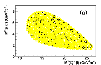
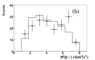
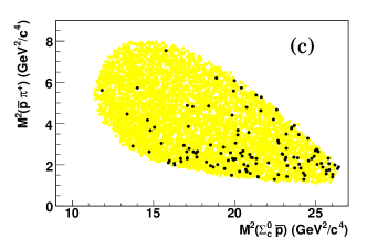
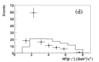
Figure 2: (a) Dalitz plot and (b) $M^{2}(\bar{p}\pi^{-})$ distribution for $\bar{B}^{0}\to\Sigma_{c}^{++}\bar{p}\pi^{-}$. (c) Dalitz plot and (d) $M^{2}(\bar{p}\pi^{+})$ distribution for $\bar{B}^{0}\to\Sigma_{c}^{0}\bar{p}\pi^{+}$. Points with error bars indicate the data, and histograms are the decays simulated according to three-body phase space.

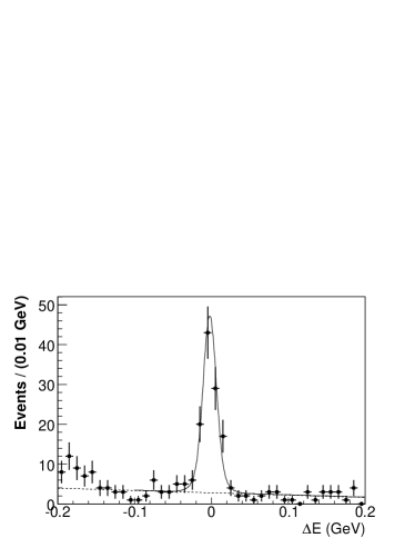
Figure 3: $\Delta{E}$ distribution for the $\bar{B}^{0}\to\Lambda_{c}^{+}\bar{p}\pi^{+}\pi^{-}$ events in the $M_{\rm bc}$ signal region with $2.447\,\rm{GeV}/c^{2}<M(\Lambda_{c}^{+}\pi^{\pm})<2.461\,\rm{GeV}/c^{2}$. The curves indicate the fit with a double Gaussian for the signal and a linear background.

Figure 4 shows (a) the $\bar{p}\pi^{+}$ mass, (b) $\cos\theta_{p}$ and (c) $\Sigma_{c}^{0}\pi^{+}$ mass distributions for the selected $\bar{B}^{0}\to\Sigma_{c}^{0}\bar{p}\pi^{+}$ events. Here, $\cos\theta_{p}$ is the cosine of the angle between the $\bar{p}$ momentum and the direction opposite to the $B$ momentum in the $\bar{p}\pi^{+}$ rest frame. The shaded histograms indicate the distributions for the background discussed above. The background shapes are obtained by fits to the data in the sideband region $|\Delta{E}|<0.1\,{\rm GeV}$ and $5.26\,{\rm GeV}/c^{2}<M_{\rm bc}<5.29\,{\rm GeV}/c^{2}$ outside the $B$ signal region, and the yield is fixed to 17 events. Here, the $M(\bar{p}\pi^{+})$ distribution is parameterized by the function $P_{\rm bkg}(M)=c\cdot\sqrt{t_{\rm min}\cdot t_{\rm max}}\cdot(1+c_{1}\cdot t_{\rm min})(1+c_{2}\cdot t_{\rm max})$ with $t_{\rm min}=(M^{2}-M^{2}_{\rm min})$ and $t_{\rm max}=(M^{2}_{\rm max}-M^{2})$. $M_{\rm min}$ and $M_{\rm max}$ are the minimum and maximum masses. The variable $c$ is a normalization constant, and $c_{1}$ and $c_{2}$ are shape parameters. The $\cos\theta_{p}$ distribution is modeled by a second-order Chebyshev polynomial.

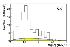
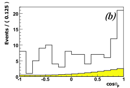
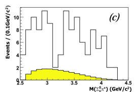
Figure 4: Data distributions for (a) $M(\bar{p}\pi^{+})$, (b) $\cos\theta_{p}$ and (c) $M(\Sigma_{c}^{0}\pi^{+})$. The shaded histograms indicate the normalized background.

We find a significant structure in the $\bar{p}\pi^{+}$ mass distribution, and a forward peak in the $\cos\theta_{p}$ distribution, and a low mass $\Sigma_{c}^{0}\pi^{+}$ enhancement, denoted as $(\Sigma_{c}^{0}\pi^{+})_{\rm X}$. The $\bar{p}\pi^{+}$ mass structure has a mass near $1.5\,{\rm GeV}/c^{2}$ and a width of about $0.3\,{\rm GeV}$. We denote it as $\bar{N}^{0}$, and investigate its characteristics in detail. In order to describe the $\bar{p}\pi^{+}$ mass structure, which is not explained by a simple phase space non-resonant $\bar{B}^{0}\to\Sigma_{c}^{0}\bar{p}\pi^{+}$ decay, we consider an intermediate two-body decay $\bar{B}^{0}\to\Sigma_{c}^{0}\bar{N}^{0}$ with a resonant state ${\bar{N}}^{0}\to{\bar{p}}\pi^{+}$. However, we still cannot reproduce the forward $\cos\theta_{p}$ peak and the $\Sigma_{c}^{0}\pi^{+}$ low mass structure with these two modes only. Therefore, we introduce one additional mode $\bar{B}^{0}\to(\Sigma^{0}_{c}\pi^{+})_{\rm X}\,\bar{p}$ to account for the observed features. As the low mass $\Sigma_{c}^{0}\pi^{+}$ structure is close to threshold, it produces a forward peak in the $\cos\theta_{p}$ distribution. In the low $\Sigma_{c}^{0}\pi^{+}$ mass region, we search for known $\Sigma_{c}^{0}\pi^{+}$ resonant states [18] in finer mass bins, but find no signals. So far, there is no good candidate to interpret this broad structure as a resonance. Therefore we assume that there is a threshold mass enhancement with a mass of $2800\,{\rm MeV/}c^{2}$ and a width of $350\,{\rm MeV}$ obtained from a fit to the $\Sigma_{c}^{0}\pi^{+}$ mass distribution using a relativistic Breit-Wigner (S-wave) function.

Figure 5 compares binned Probability Density Functions (PDF) of the MC simulated events for the three assumed decay modes. The histograms show the PDFs for (a) the $M(\bar{p}\pi^{+})$, (b) $\cos\theta_{p}$ and (c) the $M(\Sigma_{c}^{0}\pi^{+})$ distributions. The solid histograms show the distributions of the mode $\bar{B}^{0}\to\Sigma_{c}^{0}\bar{N}^{0}$, assuming a P-wave relativistic Breit-Wigner amplitude with a mass of $1530\,{\rm MeV/}c^{2}$ and a width of $340\,{\rm MeV}$.

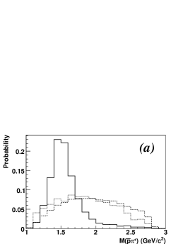
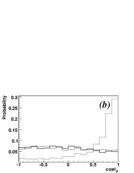
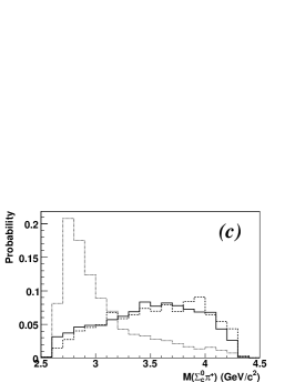
Figure 5: Binned probability distributions of (a) $M(\bar{p}\pi^{+})$, (b) $\cos\theta_{p}$ and (c) $M(\Sigma_{c}^{0}\pi^{+})$, where we compare MC simulated distributions for $\bar{B}^{0}\to\Sigma_{c}^{0}\bar{N}^{0}$ (solid lines), $\bar{B}^{0}\to\Sigma_{c}^{0}\bar{p}\pi^{+}$ (dashed lines), and $\bar{B}^{0}\to(\Sigma^{0}_{c}\pi^{+})_{\rm X}\,\bar{p}$ (dotted lines). We make a simultaneous fit to the distributions in (a) and (b).

To determine the $N^{0}$ mass, width and the yields of the three modes, we perform a maximum likelihood fit to the observed $M({\bar{p}}\pi^{+})$ and $\cos\theta_{p}$ distributions shown in Fig. 4. These two distributions are sufficient to fully describe the three-body decay $\bar{B}^{0}\to\Sigma_{c}^{0}\bar{p}\pi^{+}$. To model the observed distribution, we construct a function $F(M(\bar{p}\pi^{+}),\cos\theta_{p})$ from the sum of PDFs of the three decay modes and the background.

$$\begin{split}F=\nu_{1}P_{\bar{B}^{0}\to\Sigma_{c}^{0}\bar{N}^{0}}+\nu_{2}P_{\bar{B}^{0}\to(\Sigma_{c}^{0}\pi^{+})_{\rm X}\,\bar{p}}\\ +\nu_{3}P_{\bar{B}^{0}\to\Sigma_{c}^{0}\bar{p}\pi^{+}}+\nu_{4}P_{\rm bkg},\end{split}$$

where $P_{i}$ denotes a product of the normalized PDFs, $Q_{i}(M(\bar{p}\pi^{+}))$ (20 bins) and $R_{i}(\cos\theta_{p})$ (16 bins), and $\nu_{i}$ stands for the yield of the $i$-th mode. We plot $Q(M(\bar{p}\pi^{+}))$ and $R(\cos\theta_{p})$ distributions from the detector MC simulation for $\bar{B}^{0}\to(\Sigma^{0}_{c}\pi^{+})_{\rm X}\,\bar{p}$ and $\bar{B}^{0}\to\Sigma_{c}^{0}\bar{p}\pi^{+}$ modes, as shown in Figs 5(a) and (b), respectively. For the $\bar{B}^{0}\to\Sigma_{c}^{0}\bar{N}^{0}$ mode, we use the MC simulated $R(\cos\theta_{p})$ distribution and a Breit-Wigner for $Q(M({\bar{p}}\pi^{+}))$ with the ${\bar{N}}^{0}$ mass and width ($m_{R}$, $\Gamma$) as free parameters. A small systematic error due to the use of the $Q(M({\bar{p}}\pi^{+}))$ distribution without the MC detector simulation is discussed later. We use a P-wave (S-wave) relativistic Breit-Wigner shape.

$$BW_{P}(m^{2})=\frac{p^{2}}{(m^{2}-m_{R}^{2})^{2}+m_{R}^{2}{\Gamma^{2}(m)}}{\left[\frac{B(p)}{B(p_{0})}\right]}^{2},$$

$$BW_{S}(m^{2})=\frac{m_{R}\Gamma(m)}{[(m^{2}-{m_{R}}^{2})^{2}+{m_{R}}^{2}\Gamma^{2}(m)]},$$

$$\Gamma(m)=\left(\frac{p}{p_{0}}\right)^{2L+1}\left(\frac{m_{R}}{m}\right)\Gamma_{0}{\left[\frac{B(p)}{B(p_{0})}\right]^{2}}.$$

Here $m$ is the mass of the $\bar{p}\pi^{+}$ system, and $m_{R}$ is the nominal $\bar{N}^{0}$ mass, and $\Gamma(m)$ is the width. The variable $p$ is the momentum of a daughter particle in the $\bar{N}^{0}$ rest frame, and $p_{0}$ is that for the nominal $\bar{N}^{0}$ mass. $B(p)=1/{\sqrt{1+(Rp)^{2}}}$ is the Blatt-Weisskopf form factor [19]. The value $R$, called the centrifugal barrier penetration factor, is set to $3\,{\rm(GeV}/c)^{-1}$ for a P-wave, and is zero for an S-wave. $L$ indicates the orbital angular momentum. For the S-wave Breit-Wigner amplitude [20] we use $\Gamma(m)$ with $m=m_{R}$ and $L=0$ to parameterize the smooth shape near the mass threshold.

We define an extended unbinned likelihood with coarse bins, and carry out a maximum likelihood fit.

$$L=\frac{e^{-(\nu_{1}+\nu_{2}+\nu_{3}+\nu_{4})}}{N!}\prod F(m_{R},\Gamma,\nu_{1},\nu_{2},\nu_{3},\nu_{4})$$

We fit the ${\bar{N}}^{0}$ mass and width $(m_{R},\Gamma)$ and the yields $\nu_{1},\nu_{2}$ and $\nu_{3}$ as free parameters, while the background yield $\nu_{4}$ is fixed to 17 events. Table 1 summarizes the fit results with various model assumptions. We calculate the statistical significance from the quality -2${\rm ln}({L}_{0}/{L}_{\rm max})$, where $L_{\max}$ is the maximum likelihood returned from the fit, and $L_{0}$ is the likelihood with the signal yield fixed to zero, and taking into account the reduction of the degrees of freedom. We obtain a significance of 7.0$\,\sigma$ for the $\bar{B}^{0}\to\Sigma_{c}^{0}\bar{N}^{0}$ contribution. The signal in the mode $\bar{B}^{0}\to(\Sigma^{0}_{c}\pi^{+})_{\rm X}\,\bar{p}$ has a statistical significance of 4.6$\,\sigma$, while that for $\bar{B}^{0}\to\Sigma_{c}^{0}\bar{p}\pi^{+}$ is not significant (0.8 $\sigma$). Here, we calculate the goodness-of-fit from the likelihood ratio $\lambda$ [18],

$$\begin{split}\chi^{2}\approx-2{\rm ln}\lambda=2\sum_{j=1}^{36}[{\cal F}_{j}(m_{R},\Gamma,\nu_{1},\nu_{2},\nu_{3},\nu_{4})-F_{j}\\ +F_{j}{\rm ln}(\frac{F_{j}}{{\cal F}_{j}(m_{R},\Gamma,\nu_{1},\nu_{2},\nu_{3},\nu_{4})})],\end{split}$$

where $F_{j}$ and ${\cal F}_{j}$ are the observed and the fitted yields, respectively, in the $j$-th bin: $j=1,20$ for 20 bins in $Q(M(\bar{p}\pi^{+}))$ and $j=21,36$ for 16 bins in $R(cos\theta_{p})$.

The small contribution ($\nu_{3}=-11\pm 10$) can be understood from Fig. 5. The mode $\bar{B}^{0}\to\Sigma_{c}^{0}\bar{p}\pi^{+}$ has a broad $\bar{p}\pi^{+}$ mass distribution similar to $\bar{B}^{0}\to(\Sigma^{0}_{c}\pi^{+})_{\rm X}\,\bar{p}$, while it does not reproduce the forward $\cos\theta_{\bar{p}}$ peak. On the other hand, the $\bar{B}^{0}\to\Sigma_{c}^{0}\bar{N}^{0}$ mode can reproduce the ${\bar{p}}\pi^{+}$ mass bump structure and the uniform $\cos\theta_{\bar{p}}$ distribution. Hence, we fix $\nu_{3}=0$ in the subsequent fit and the uncertainty of this contribution is taken into account in the systematic error.

Table 1: Summary of the simultaneous fits to the $M(\bar{p}\pi^{+})$ and $\cos\theta_{\bar{p}}$ distributions with the three decay modes $\bar{B}^{0}\to\Sigma_{c}^{0}\bar{N}^{0}$, $\bar{B}^{0}\to\Sigma_{c}^{0}\bar{p}\pi^{+}$ and $\bar{B}^{0}\to(\Sigma^{0}_{c}\pi^{+})_{\rm X}\,\bar{p}$. (a) - (d) represent fits with various assumed contributions. Here, we show the fit results with the P-wave assumption, as we find no significant difference from the S-wave assumption.

Decay mode	(a)	(b)	(c)	(d)	Signif.
$\bar{B}^{0}\to\Sigma_{c}^{0}\bar{N}^{0}$	free	free	free	0	7.0
$\bar{B}^{0}\to(\Sigma^{0}_{c}\pi^{+})_{\rm X}\,\bar{p}$	free	free	0	free	4.6
$\bar{B}^{0}\to\Sigma_{c}^{0}\bar{p}\pi^{+}$	free	0	free	free	0.8
$\chi^{2}$/ndf	31.7/31	32.4/32	52.8/32	88.4/34

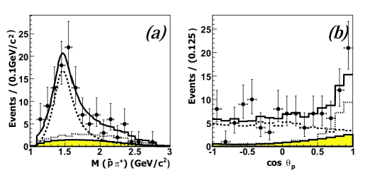
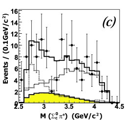
Figure 6: Simultaneous fit to (a) $M({\bar{p}}\pi^{+})$ and (b) $\cos\theta_{p}$ distributions with a P-wave Breit-Wigner. The points with error bars are the data, and the curves are the contributions from $\bar{B}^{0}\to\Sigma_{c}^{0}\bar{N}^{0}$ (dashed), $\bar{B}^{0}\to(\Sigma^{0}_{c}\pi^{+})_{\rm X}\,\bar{p}$ (dotted), the background (shaded) and their sum (solid). (c) $M(\Sigma_{c}^{0}\pi^{+})$ distribution, where the curves represent their contributions obtained by the fit to (a) and (b).

Figure 6 shows the results of a fit to (a) the $M({\bar{p}}\pi^{+})$ and (b) $\cos\theta_{\bar{p}}$ distributions under the P-wave assumption. The data are the points with error bars. The curves are the contributions from $\bar{B}^{0}\to\Sigma_{c}^{0}\bar{N}^{0}$ (dashed), $\bar{B}^{0}\to(\Sigma^{0}_{c}\pi^{+})_{\rm X}\,\bar{p}$ (dotted), the background (shaded) and their sum (solid). We obtain yields of ($70\pm 11$) and ($32\pm 9$) for the modes $\bar{B}^{0}\to\Sigma_{c}^{0}\bar{N}^{0}$ and $\bar{B}^{0}\to(\Sigma^{0}_{c}\pi^{+})_{\rm X}\,\bar{p}$, respectively. Figure 6(c) shows that the $M(\Sigma_{c}^{0}\pi^{+})$ distribution is consistently represented by the fitted parameters even though the $M(\Sigma_{c}^{0}\pi^{+})$ distribution is not included in the fit.

Table 2: The fitted ${\bar{N}}^{0}$ mass and width with relativistic S-wave and P-wave Breit-Wigners. The first errors are statistical and the second are systematic including the uncertainties in the yields of $\bar{B}^{0}\to\Sigma_{c}^{0}\bar{p}\pi^{+}$ and the background, and the assumption of a low mass $(\Sigma_{c}^{0}\pi^{+})_{\rm X}$ structure.

Item	Yield	Mass	$\Gamma$	$\chi^{2}$/ndf
	Events	$\rm{MeV}/c^{2}$	$\rm{MeV}$
S-wave	$71\pm 11\pm 10$	$1473\pm 31\pm 2$	$315\pm 72\pm 53$	32.9/32
P-wave	$70\pm 11\pm 10$	$1516\pm 29\pm 14$	$365\pm 97\pm 90$	32.4/32
$\Sigma_{c}^{0}\pi^{+}$ sys.	$\pm 5$	$\pm 8$	$\pm 50$

Table 2 compares the fit results for the ${\bar{N}}^{0}$ yield, mass and width with P-wave and S-wave assumptions. The fitted yields are found to be comparable with each other, while the mass and width show a systematic difference. We estimate systematic errors by varying the fitted yields by $\pm\sigma$ for the background ($\pm 3$) and $\bar{B}^{0}\to\Sigma_{c}^{0}\bar{p}\pi^{+}$ ($\pm 11$), and by taking into account the uncertainty in modeling the low mass $(\Sigma_{c}^{0}\pi^{+})_{\rm X}$ structure as discussed in the following.

The simulated $R(\cos\theta_{p})$ distribution for $\bar{B}^{0}\to\Sigma_{c}^{0}\bar{N}^{0}$ is almost flat, as the generated $\cos\theta_{p}$ distribution is uniform for $P$- and $S$-waves. However, the $R(cos\theta_{p})$ distribution is slightly affected by the assumed BW parameters due to efficiency changes in $\cos\theta_{p}$. We study the systematics of the fitted ${\bar{N}}^{0}$ mass and width due to the assumption on $R(\cos\theta_{p})$, by changing the mass and the width in EvtGen in ranges between $1400\,{\rm MeV}/c^{2}$ and $1620\,{\rm MeV}/c^{2}$, and between $200\,{\rm MeV}$ and $450\,{\rm MeV}$, respectively. We find variations of $\pm 1\,{\rm MeV}/c^{2}$ in the fitted mass and $\pm 5\,{\rm MeV}/c^{2}$ in the width. We also study the systematic errors due to the parameterization of the $(\Sigma_{c}^{0}\pi^{+})$ low mass structure. Instead of assuming a model with a single Breit-Wigner $(\Sigma_{c}^{0}\pi^{+})_{\rm X}$, we consider a combination of known states $\Lambda_{c}^{*}\to\Sigma_{c}(2455)^{0}\pi^{+}$; $\Lambda_{c}^{+}(2625)$ ($\Gamma_{\rm total}<1.9\,{\rm MeV}$) [18], $\Lambda_{c}^{+}(2765)\to\Lambda_{c}^{+}\pi^{+}\pi^{-}$ ($\Gamma\sim 50\,{\rm MeV}/c^{2}$), $\Lambda_{c}^{+}(2880)$ ($\Gamma=5.8\pm 1.3\,{\rm MeV}$), and $\Lambda_{c}^{+}(2940)$ ($\Gamma=13^{+28}_{-9}\,{\rm MeV}$). Here we use the partial widths for $\Sigma_{c}^{0}\pi^{+}$ decay of the last three states given by Ref. [21]. We make a fit to the $\bar{N}^{0}$ mass, width and the yield of $\bar{B}^{0}\to\Sigma_{c}^{0}\bar{N}^{0}$ with the individual $\Lambda_{c}^{*+}$ yields floated and with the background fixed as mentioned previously. We obtain $N({\bar{p}}\pi^{+})$ mass and width values in good agreement with those obtained by the fit with the $\bar{B}^{0}\to(\Sigma^{0}_{c}\pi^{+})_{\rm X}\,\bar{p}$ model.

The branching fraction product ${\cal B}$($\bar{B}^{0}\to\Sigma_{c}^{0}\bar{N}^{0}$)$\times{\cal B}(\bar{N}^{0}\to\bar{p}\pi^{+})$ is calculated as $N_{s}/(N_{B\bar{B}}\cdot\epsilon\cdot CF\cdot{\cal B}_{\Lambda_{c}^{+}\to pK^{-}\pi^{+}})$ assuming $N_{B^{+}B^{-}}=N_{B^{0}\bar{B}^{0}}$. For $N_{s}$ we use the P-wave yield in Table 2 as it gives a better confidence level than an S-wave fit. We use $N_{B\bar{B}}=(387.7\pm 4.8)\times 10^{6}$ for the integrated luminosity of 357 fb^-1, and the signal efficiency $\epsilon=(5.18\pm 0.13$)% from the MC simulation of $\bar{B}^{0}\to\Sigma_{c}^{0}\bar{N}^{0}$. We apply a correction factor $CF=(86.7\pm 7.9)$%, which takes into account the systematic difference in particle identification (PID) between data and MC simulation. Correction factors for proton, kaon and pion tracks are determined from a comparison of data and MC simulation for large samples of $D^{*+}\to D^{0}(K\pi)\pi^{+}$ and $\Lambda\to p\pi^{-}$ decays. The overall PID correction factor is then calculated as a linear sum over the six tracks for the selected $B$ signal events. We assign an error of 7.2% due to track reconstruction efficiency for the six charged tracks in the final state. The systematic error on the branching fraction arising from a quadratic sum of the uncertainties on $N_{B\bar{B}}$, the signal efficiency $\epsilon$, and particle identification $CF$ and track reconstruction, is found to be 12%. Including the systematic error in the $\bar{B}^{0}\to\Sigma_{c}^{0}\bar{N}^{0}$ yield, we arrive at the total systematic uncertainty in the branching fraction of 17.6 %. Thus, we obtain the branching fraction product of ${\cal B}(\bar{B}^{0}\to\Sigma_{c}(2455)^{0}\bar{N}^{0})\times{\cal B}(\bar{N}^{0}\to\bar{p}\pi^{+})$=($0.80\pm 0.15\rm{(stat.)}\pm 0.14\rm{(syst.)}\pm 0.21$)$\times 10^{-4}$, and a significance of 6.1 standard deviations including systematics. The last error is due to an uncertainty in ${\cal B}(\Lambda_{c}^{+}\to pK^{-}\pi^{+})=(5.0\pm 1.3)\%$ [18].

Next, we investigate goodness-of-fits with the masses and widths fixed to representative values for $N({\bar{p}}\pi^{+})$ states [18], and by floating the yields for $\bar{B}^{0}\to\Sigma_{c}^{0}\bar{N}^{0}$ and $\bar{B}^{0}\to(\Sigma^{0}_{c}\pi^{+})_{\rm X}\,\bar{p}$. The fit results are summarized in Table 3. Here $L_{2I,2S}$ stands for a resonance of isospin $I$ and spin $S$ with an orbital angular momentum of $L$=S, P and D for $L$=0, 1 and 2, respectively. We exclude $\Delta$ states such as $\Delta(1600)P_{33}$ and $\Delta(1620)S_{31}$, as we have no significant structure in the $\bar{p}\pi^{-}$ mass distribution in $\bar{B}^{0}\to\Sigma_{c}^{++}\bar{p}\pi^{-}$ decay. The fits favor $N(1440)P_{11}$ and $N(1535)S_{11}$, while they disfavor $N(1520)D_{13}$ and $N(1650)S_{11}$. In the decay $\bar{B}^{0}\to\Sigma^{0}_{c}\bar{N}^{0}$ (assuming $S(\Sigma^{0}_{c})=\frac{1}{2}$), one expects a uniform $\cos\theta_{p}$ distribution for the $N(1440)P_{11}$ state, $N(1535)S_{11}$ state and $N(1650)S_{11}$ state, and a $(1+3\cos^{2}\theta)$ distribution for the $N(1520)D_{13}$ state. As shown in Fig. 6(b), the distribution has a peak only in the forward direction, which is well reproduced by the mode $\bar{B}^{0}\to(\Sigma^{0}_{c}\pi^{+})_{\rm X}\,\bar{p}$. The remaining uniform distribution is due to $\bar{B}^{0}\to\Sigma_{c}^{0}\bar{N}^{0}$. Thus, the observed $\cos\theta_{\bar{p}}$ distribution is consistent with both, $\bar{N}(1440)P_{11}$ and $\bar{N}(1535)S_{11}$ states, with a preference for the former due to the width of the state.

Table 3: Results of the fits using the parameters of known $N({\bar{p}}\pi^{+})$ resonances [18].

States		Mass	$\Gamma$	$\Sigma_{c}^{0}\bar{N}^{0}$	$(\Sigma_{c}^{0}\pi^{+})_{X}\bar{p}$	$\chi^{2}$/ndf
		${\rm MeV}/c^{2}$	$~{}{\rm MeV}$	Events	Events
N(1440)	$P_{11}$	1440	300	$65\pm 10$	$39\pm 9$	37.6/34
N(1520)	$D_{13}$	1520	115	$46\pm 9$	$53\pm 10$	53.5/34
N(1535)	$S_{11}$	1535	150	$58\pm 10$	$43\pm 10$	40.1/34
N(1650)	$S_{11}$	1655	165	$44\pm 10$	$55\pm 11$	74.2/34

Finally, we try to perform a fit with an incoherent sum of the two Breit-Wigners, as we find that the fit results favor $N(1440)P_{11}$ and $N(1535)S_{11}$, and both give a distribution uniform in $\cos\theta_{p}$. Figure 7 shows the result of a fit to (a) the $M(\bar{p}\pi^{+})$ and (b) $\cos{\theta}_{\bar{p}}$ distributions, where the $N$ masses and widths are fixed to the values in Ref. [18], and the individual yields are floated. The histograms show the contributions from $N(1440)$ (solid), $N(1535)$ (dashed) states, $\bar{B}^{0}\to(\Sigma^{0}_{c}\pi^{+})_{\rm X}\,\bar{p}$ (dotted), and the background (shaded). The yields are $(37\pm 12)$ for the $N(1440)$ and $(30\pm 11)$ for the $N(1535)$, while the $\bar{B}^{0}\to(\Sigma^{0}_{c}\pi^{+})_{\rm X}\,\bar{p}$ yield is $(35\pm 9)$. We obtain the goodness of fit $\chi^{2}$/ndf=30.3/33, which indicates a slight preference (by 2.7 $\sigma$) for a mixed state of $N(1440)$ and $N(1535)$ [18].

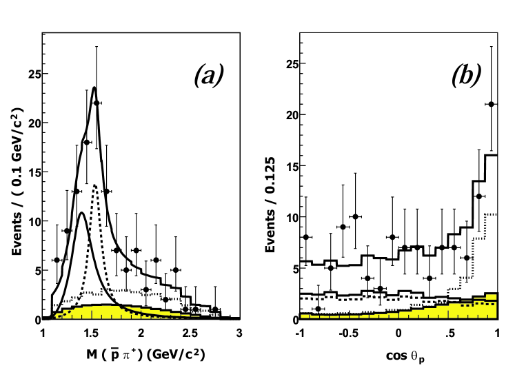
Figure 7: Simultaneous fit to the $M(\bar{p}\pi^{+})$ and $\cos{\theta}_{\bar{p}}$ distributions with the $N(1440)P_{11}$ and $N(1535)S_{11}$ Breit-Wigners. The histograms indicate the contributions from the $P_{11}$ (solid) and $S_{11}$ (dashed) states, $\bar{B}^{0}\to(\Sigma^{0}_{c}\pi^{+})_{\rm X}\,\bar{p}$ (dotted), and the background (shaded).

In summary, we study the three-body decay $\bar{B}^{0}\rightarrow\Sigma_{c}(2455)^{0}\bar{p}\pi^{+}$ with the same data set used for the analysis of the four-body decay $\bar{B}^{0}\rightarrow\Lambda_{c}^{+}\bar{p}\pi^{+}\pi^{-}$ [1]. We observe a broad $\bar{p}\pi^{+}$ mass structure near $1.5\,{\rm GeV}/c^{2}$, and a uniform $\cos{\theta}_{\bar{p}}$ distribution with a sharp forward peak. To explain these structures, we find that contributions from an intermediate two-body decay $\bar{B}^{0}\to\Sigma_{c}^{0}\bar{N}^{0}$, non-resonant three-body decay $\bar{B}^{0}\to\Sigma_{c}^{0}\bar{p}\pi^{+}$ and a low mass structure near threshold $\bar{B}^{0}\to(\Sigma^{0}_{c}\pi^{+})_{\rm X}\,\bar{p}$ are needed. We perform a simultaneous fit to the $M(\bar{p}\pi^{+})$ and $\cos{\theta}_{\bar{p}}$ distributions with those three modes, and determine the yield and the relativistic Breit-Wigner parameters of the ${\bar{N}}^{0}$ state for $\bar{B}^{0}\to\Sigma_{c}^{0}\bar{N}^{0}$. We obtain the branching fraction product of ${\cal B}(\bar{B}^{0}\to\Sigma_{c}(2455)^{0}\bar{N}^{0})\times{\cal B}(\bar{N}^{0}\to\bar{p}\pi^{+})$=($0.80\pm 0.15\rm{(stat.)}\pm 0.14\rm{(syst.)}\pm 0.21$)$\times 10^{-4}$ with a signal significance of 6.1 standard deviations including systematics. The fitted mass and width are consistent with $\bar{N}(1440)$$P_{11}$ and $\bar{N}(1535)S_{11}$; both states also produce a uniform helicity distribution that is in good agreement with the data. The structure is also consistent with an interpretation in terms of an admixture of these two states.

ACKNOWLEDGMENT

We thank the KEKB group for excellent operation of the accelerator, the KEK cryogenics group for efficient solenoid operations, and the KEK computer group and the NII for valuable computing and Super-SINET network support. We acknowledge support from MEXT and JSPS (Japan); ARC and DEST (Australia); NSFC (China); DST (India); MOEHRD, KOSEF and KRF (Korea); KBN (Poland); MES and RFAAE (Russia); ARRS (Slovenia); SNSF (Switzerland); NSC and MOE (Taiwan); and DOE (USA).

References

[1] K.S. Park et al. (Belle Collaboration),
Phys. Rev. D 75, 011101 (2007).
[2]
N. Gabyshev et al. (Belle Collaboration),
Phys. Rev. D 66, 091102(R) (2002).
[3]
N. Gabyshev et al. (Belle Collaboration),
Phys. Rev. Lett. 90, 121802 (2003).
[4]
N. Gabyshev et al. (Belle Collaboration),
Phys. Rev. Lett. 97, 202003 (2006).
[5]
N. Gabyshev et al. (Belle Collaboration),
Phys. Rev. Lett. 97, 242001 (2006).
[6] X. Fu et al. (CLEO Collaboration), Phys. Rev. Lett. 79, 3125 (1997).
[7]
S.A. Dytman et al. (CLEO Collaboration), Phys. Rev. D 66, 091101(R) (2002).
[8]
H. Kichimi, Nucl. Phys. B Proc. Suppl. 142, 197 (2005).
[9] M. Kobayashi and K. Maskawa, Prog. Theor. Phys. 49, 652 (1973).
[10] M. Jarfi et al., Phys. Lett. B 237, 513 (1990);
M. Jarfi et al., Phys. Rev. D 43, 1599 (1991);
N. Deshpande, J. Trampetic and A. Soni, Mod. Phys. Lett. 3A, 749 (1988).
[11] V. Chernyak and I. Zhitnisky, Nucl. Phys. B 345, 137 (1990).
[12]
H.Y. Cheng and K.C. Yang,
Phys. Rev. D 67, 034008 (2003).
[13]
S. Kurokawa and E. Kikutani,
Nucl. Instr. Meth. A 499, 1 (2003),
and other papers included in this Volume.
[14]
A. Abashian et al. (Belle Collaboration), Nucl. Instr. and
Meth. A 479, 117 (2002).
[15]
D.J. Lange, Nucl. Instr. and Meth. A 462, 152 (2001).
[16]
The detector response is simulated using GEANT: R. Brun et al.,
GEANT 3.21, CERN Report DD/EE/84-1 (1984).
[17]
E. Nakano,
Nucl. Instr. and Meth. A 494, 402 (2002).
[18]
W.-M. Yao et al. (Particle Data Group), J. Phys. G 33, 1 (2006) (URL:http://pdg.lbl.gov).
[19]
J. Blatt and V. Weisskopf, Theoretical Nuclear Physics, New York: John Wiley & Sons (1952).
[20]
H.M. Pilkuhn, The Interactions of Hadrons, Amsterdam: North-Holand Pub. Co. (1967).
[21]
R. Mizuk et al. (Belle collaboration),
Phys. Rev. Lett. 98, 262001 (2007).