Dynamical thermalization and vortex formation in stirred 2D Bose-Einstein condensates

Abstract

We present a quantum mechanical treatment of the mechanical stirring of Bose-Einstein condensates using classical field techniques. In our approach the condensate and excited modes are described using a Hamiltonian classical field method in which the atom number and (rotating frame) energy are strictly conserved. We simulate a $T=0$ quasi-2D condensate perturbed by a rotating anisotropic trapping potential. Vacuum fluctuations in the initial state provide an irreducible mechanism for breaking the initial symmetries of the condensate and seeding the subsequent dynamical instability. Highly turbulent motion develops and we quantify the emergence of a rotating thermal component that provides the dissipation necessary for the nucleation and motional-damping of vortices in the condensate. Vortex lattice formation is not observed, rather the vortices assemble into a spatially disordered vortex liquid state. We discuss methods we have developed to identify the condensate in the presence of an irregular distribution of vortices, determine the thermodynamic parameters of the thermal component, and extract damping rates from the classical field trajectories.

I Introduction

The experimental observation of vortex lattices in Bose-Einstein condensates (BECs) Madison00 ; Madison01b ; Abo-Shaeer01 ; Abo-Shaeer02 ; Raman01 ; Haljan01a ; Hodby02 has stimulated intense theoretical interest and debate over the mechanisms involved in vortex formation. While vortex lattices had previously been observed in superconductors and superfluid Helium, dilute gas BECs offer the possibility of a quantitative description of the formation process using tractable theory. The experiments can be divided broadly into two categories: (i) A thermal gas rotating in an axially symmetric trap is evaporatively cooled and condenses into a rotating lattice Haljan01a ; (ii) A low temperature condensate ($T\ll T_{\mathrm{C}}$ ) is rotationally stirred, and vortices then nucleate and form a vortex lattice Madison00 ; Madison01b ; Abo-Shaeer01 ; Abo-Shaeer02 ; Raman01 ; Hodby02 . The first category of experiment is conceptually simplest, and the origin of dissipative processes is well understood Penckwitt02 ; Williams2002a ; Bradley08 . The second category of experiment is the subject of this paper, and as observed by a number of groups, has more complicated phenomenology. We shall concentrate on a typical, representative example, in which the condensate is initially in the interacting ground state of a cylindrically symmetric harmonic trap at a temperature very close to $T=0$. Stirring is implemented by distorting the trap to elliptical symmetry, and rotating it at the frequency of the condensate quadrupole mode. This excites a dynamical instability in which the condensate is transformed into a turbulent state, which later evolves into a rotating state containing a regular vortex lattice.

This process of vortex lattice formation by stirring provides a unique testbed for dynamical theories of cold bosonic gases, as noted by other authors Kasamatsu03 . Beginning from a well characterised initial state, the application of a simply defined experimental procedure causes a violent transformation into a highly excited and disordered state, from which an ordered state subsequently emerges. The workhorse of BEC theory, the Gross-Pitaevskii equation (GPE), can provide a good dynamical description of $T=0$ condensates, and has given a very good understanding of the initiation of the dynamical instability Sinha01 ; Recati01 ; Kasamatsu03 ; Parker06 . The subsequent evolution into a highly excited state is clearly beyond the validity regime of pure GP theory. Tsubota et al. Tsubota02a recognised the need for a new theoretical framework after noting that dissipation is required to evolve an initially non-rotating GPE ground state into a state in equilibrium with the stirrer. They postulated that a rotating thermal cloud develops to provide this dissipation (see also Ref. Penckwitt02 ), and modelled its effects by adding a phenomenological damping term to the GPE Choi98a , later justified Kasamatsu03 on the basis of the formalism of Jackson and Zaremba Jackson2001 . Further calculations employing the GPE were performed by Parker et al. Parker06b ; Parker05a , and these 2D simulations gave rise to crystallization of a low energy vortex lattice, in conflict with earlier simulations of the GPE in 2D Feder01a ; Lundh03 that did not exhibit lattice formation. It is of interest to identify the origin of this discrepancy and to determine the nature of the final state to be expected in stirring experiments of 2D Bose gases.

In this paper we apply classical field theory, a representation of many-body physics capable of modelling the dynamical behaviour of both the condensate and excited states of the matter field. The formalism for classical field theory has been developed recently in a number of papers Steel98 ; Davis01 ; Sinatra01 ; Sinatra02 ; Gardiner02 ; Blakie05 ; Bradley08 , and it has been used to describe several phenomena where thermal fluctuations play a critical role in determining the dynamical behaviour of the system, including: the condensation transition Blakie05 ; Bradley08 , effects of critical fluctuations on the transition temperature Davis06 , activation of vortices in quasi-2D systems Simula06 ; Simula2008a ; Bisset2008a , collapse dynamics of attractive Bose gases Wuster2007a , and coherence properties of spinor condensates Gawryluk2007a . Lobo et al. Lobo04 have used a version of classical field theory to describe vortex lattice formation by stirring, and their results indicate that the thermal field component generated provides the damping necessary for the lattice to form. Here we will apply an implementation of classical field theory which conserves particle number and rotating frame energy, and uses a basis choice and numerical method that has appropriate boundary conditions and is free from numerical artifacts. This allows us to provide a detailed and quantitative description of the thermalization of the condensate, and the nucleation and motional damping of vortices which is responsible for lattice formation. We find that the system relaxes to a state containing a disordered distribution of vortices, in thermal and rotational equilibrium with a cloud of thermal atoms generated by the stirring process.

II System and equations of motion

The theory of the trapped Bose gas can be written in terms of the second quantized Hamiltonian for the field operator

$$\hat{\Psi}(\mathbf{x})=\sum_{n}\hat{a}_{n}\phi_{n}(\mathbf{x}),$$ (1)

where the operators satisfy bosonic commutation relations $[\hat{a}_{n},\hat{a}_{m}^{\dagger}]=\delta_{nm}$, and the modes $\phi_{n}(\mathbf{x})$ are any complete orthonormal basis. In the s-wave interaction regime the Hamiltonian for the system is given by

$$H = \int d^{3}\mathbf{x}\;\hat{\Psi}^{\dagger}(\mathbf{x})H_{\mathrm{sp}}\hat{\Psi}(\mathbf{x})$$ (2)

$$+\frac{U}{2}\int d^{3}\mathbf{x}\;\hat{\Psi}^{\dagger}(\mathbf{x})\hat{\Psi}^{\dagger}(\mathbf{x})\hat{\Psi}(\mathbf{x})\hat{\Psi}(\mathbf{x})$$

where $U=4\pi\hbar^{2}a/m$, $a$ is the scattering length and $m$ is the atomic mass. The single particle Hamiltonian is generally of the form $H_{\mathrm{sp}}=H^{0}_{\mathrm{sp}}+V_{\epsilon}(\mathbf{x})+\delta V(\mathbf{x},t)$ where

$$H^{0}_{\mathrm{sp}}=\frac{-\hbar^{2}\nabla^{2}}{2m}+V_{0}(\mathbf{x})-\Omega L_{z},$$ (3)

and we have expressed the single particle Hamiltonian in a frame rotating at angular frequency $\Omega$ about the $z$-axis and decomposed the external trapping potential into

$$V(\mathbf{x},t)=V_{0}(\mathbf{x})+V_{\epsilon}(\mathbf{x})+\delta V(\mathbf{x},t).$$ (4)

We have singled out $V_{0}(\mathbf{x})$ in Eqs. (3), (4) as it will be used below to define the single particle basis for the system. $V_{\epsilon}(\mathbf{x})$ is the remaining time independent potential, and any time dependent potentials present are represented by $\delta V(\mathbf{x},t)$.

II.1 The system

We consider a condensate initially at temperature $T=0$ and confined in a cylindrically symmetric harmonic trap with trapping potential

$$V_{0}(\mathbf{{\normalcolor x}})=\left(m/2\right)\left\{\omega_{r}^{2}\left(x^{2}+y^{2}\right)+\omega_{z}^{2}z^{2}\right\}.$$ (5)

The trap is deformed at time $t=0$ into an ellipse in the $xy$-plane which rotates around the $z$-axis with angular frequency $\Omega$. In the frame rotating at frequency $\Omega$, $\delta V=0$ and the trapping potential takes the form

$$V(\mathbf{x},t)=V_{0}(\mathbf{x})+V_{\epsilon}(\mathbf{x}),$$ (6)

where

$$V_{\epsilon}(\mathbf{x})=\epsilon m\omega_{r}^{2}(y^{2}-x^{2}).$$ (7)

In this paper we set the trap eccentricity to $\epsilon\equiv 0.025$ which is sufficient to excite the quadrupole instability at $\Omega\sim\omega_{r}/\sqrt{2}$ Sinha01 ; Recati01 . In this work we will always drive the system within the hydrodynamic resonance, choosing $\Omega\equiv 0.75\omega_{r}$. The sudden turn-on of the rotating potential at fixed $\epsilon,\Omega$, means that the rotating frame energy (the quantum average of Eq. (2)) is a conserved quantity of the motion.

For computational reasons we now restrict our attention to an effective two dimensional system. Such systems have been experimentally realised (e.g., Stock05 ) by setting the trapping frequency $\omega_{z}$ sufficiently high that no modes are excited in the $z$ direction. A 2D description of our system is thus valid provided that Petrov00

$$\mu+kT\ll\hbar\omega_{z},$$ (8)

where $\mu$ and $T$ are the system chemical potential and temperature respectively. Provided that the oscillator length $l_{z}=\sqrt{\hbar/m\omega_{z}}$ corresponding to the $z$ confinement greatly exceeds the s-wave scattering length $a$, the scattering is well described by the usual 3D contact potential Petrov00 , and we obtain an effective two-dimensional equation in which the collisional interaction parameter is simply rescaled to $U_{\mathrm{2D}}=2\sqrt{2\pi}\hbar^{2}a/ml_{z}$ Bradley08 ; Petrov00 . In this work we consider ²³Na atoms confined in a strongly oblate trap, with trapping frequencies $(\omega_{r},\omega_{z})=2\pi\times(10,2000)\mathrm{rad/s}$. The s-wave scattering length is $a=2.75\mathrm{nm}$ and the oscillator length $l_{z}=468\mathrm{nm}$. Having chosen appropriate parameters, in the next section we make the dimensional reduction formally rigorous by introducing an energy cutoff into the theory which excludes all excited $z$-axis modes.

II.2 Classical field theory

In projected classical field theory a cutoff energy $E_{\mathrm{R}}$ is introduced to separate the system into a low energy region (L) with single particle energies satisfying $\epsilon_{n}<E_{\mathrm{R}}$, and a high energy region (H) containing the remaining modes. Following Gardiner02 ; Gardiner03 ; Bradley08 we shall refer to these regions as the condensate and non-condensate bands, respectively. This separation is motivated by the expectation that low energy modes will be significantly occupied. Where possible it is most convenient to carry out the separation in the basis which diagonalizes the single particle Hamiltonian of the system since at high energies ($\sim E_{\mathrm{R}}$) the many-body Hamiltonian (Eq. 2) is approximately diagonal in this basis (i.e., at such an energy a cutoff imposed at a single particle energy is approximately parallel to one imposed at an energy of the interacting system).

For certain potentials an appropriate numerical quadrature method exists which also greatly expedites simulations. Any numerical representation of field theory on a computer is also subject to a restriction of the modes. In what follows we provide an explicit connection between the cutoff in our theory and our numerical implementation.

We begin by introducing the projected field operator

$$\hat{\psi}(\mathbf{x}) \equiv \sum_{n\in\mathbf{L}}\hat{a}_{n}\phi_{n}(\mathbf{x})$$ (9)

$$= {\cal P}\hat{\Psi}(\mathbf{x}),$$

where the projector is defined as

$${\cal P}f(\mathbf{x})\equiv\sum_{n\in\mathbf{L}}\phi_{n}(\mathbf{x})\int d^{3}\mathbf{y}\;\phi_{n}^{*}(\mathbf{y})f(\mathbf{y}).$$ (10)

The summation is over all modes satisfying $\epsilon_{n}\leq E_{\mathrm{R}}$, where $H^{0}_{\mathrm{sp}}\phi_{n}(\mathbf{x})=\epsilon_{n}\phi_{n}(\mathbf{x})$ defines the modes in terms of a time independent single particle Hamiltonian in the rotating frame. Choosing $E_{\mathrm{R}}<\hbar\omega_{z}$, all excited $z$-axis modes are excluded from this set. In the s-wave limit, the effective low energy Hamiltonian for the system is then given by

$$H_{\mathrm{eff}}=\int d^{2}\mathbf{x}\;\hat{\psi}^{\dagger}(\mathbf{x})H_{\mathrm{sp}}\hat{\psi}(\mathbf{x})+\frac{U_{\mathrm{2D}}}{2}\hat{\psi}^{\dagger}(\mathbf{x})\hat{\psi}^{\dagger}(\mathbf{x})\hat{\psi}(\mathbf{x})\hat{\psi}(\mathbf{x})$$ (11)

We now obtain a classical theory by making the replacement $\hat{\psi}(\mathbf{x})\to\psi(\mathbf{x})$ in $H_{\mathrm{eff}}$ to give

$$H_{\mathrm{CF}}=\int d^{2}\mathbf{x}\;\psi^{*}(\mathbf{x})H_{\mathrm{sp}}\psi(\mathbf{x})+\frac{U_{\mathrm{2D}}}{2}|\psi(\mathbf{x})|^{4}.$$ (12)

This approach is based on the high occupation condition, where it is known that classical behaviour is recovered for highly occupied bosonic modes since commutators become relatively unimportant Davis01 . We then obtain the equation of motion for the classical field via projected functional differentiation of the classical field Hamiltonian Gardiner03 :

$$i\hbar\frac{\partial\psi(\mathbf{x})}{\partial t}=\frac{\bar{\delta}H_{\mathrm{CF}}}{\bar{\delta}\psi^{*}(\mathbf{x})}.$$ (13)

The resulting equation of motion, the projected Gross-Pitaevskii equation (PGPE)

$$i\hbar\frac{\partial\psi(\mathbf{x})}{\partial t}={\cal P}\left\{\left(H_{\mathrm{sp}}+U_{\mathrm{2D}}|\psi(\mathbf{x})|^{2}\right)\psi(\mathbf{x})\right\},$$ (14)

satisfies several identities governing the evolution of total number $N=\int d^{2}\mathbf{x}\;|\psi(\mathbf{x})|^{2}$, rotating frame energy $H_{\mathrm{CF}}$, and angular momentum $\overline{L_{z}}$ Bradley05 :

$$\frac{dN}{dt} = 0,$$ (15)

$$\frac{d\overline{L_{z}}}{dt} = -\frac{i}{\hbar}\overline{L_{z}V(\mathbf{x})}+\frac{2}{\hbar}{\rm Im}\left[\int d^{2}\mathbf{x}\;\psi^{*}(\mathbf{x})\left(V_{\epsilon}(\mathbf{x})+U_{\mathrm{2D}}|\psi(\mathbf{x})|^{2}\right){\cal Q}\left\{L_{z}\psi(\mathbf{x})\right\}\right],$$ (16)

$$\frac{dH_{\mathrm{CF}}}{dt} = -\frac{2\Omega}{\hbar}{\rm Im}\left[\int d^{2}\mathbf{x}\;\psi^{*}(\mathbf{x})\left(V_{\epsilon}(\mathbf{x})+U_{\mathrm{2D}}|\psi(\mathbf{x})|^{2}\right){\cal Q}\left\{L_{z}\psi(\mathbf{x})\right\}\right],$$ (17)

where ${\cal Q}=1-{\cal P}$ is the projector orthogonal to ${\cal P}$, and the bar represents spatial averaging: $\overline{A}=\int d^{2}\mathbf{x}\;\psi^{*}(\mathbf{x})A\psi(\mathbf{x})$. The terms involving the imaginary part of an integral are boundary terms arising in the projected classical field theory. Although we work in the frame where $\delta V(\mathbf{x},t)\equiv 0$, Eqs. (14)-(17) hold for any partitioning of the time independent potential into additive parts $V_{0}(\mathbf{x})$ and $V_{\epsilon}(\mathbf{x})$ and therefore the precise choice of $V_{0}(\mathbf{x})$ defining our projector in Eq. (10) is in principle arbitrary. However, in order that we recover the formal properties of the continuous classical field theory, the boundary terms in Eqs. (16), (17) must be made to vanish. This is ensured by expanding $\psi(\mathbf{x})$ in eigenstates of $L_{z}$, which is equivalent to requiring the projection operator to have rotational symmetry: $[{\cal P},L_{z}]\equiv[{\cal Q},L_{z}]=0$. We then have ${\cal Q}\left\{L_{z}\psi(\mathbf{x})\right\}\equiv 0$ and we see that our choice of $V_{0}(\mathbf{x})=m\omega_{r}^{2}r^{2}/2$ given in Sec. II.1 generates the appropriate rotating frame classical field theory. The remaining potential $V_{\epsilon}(\mathbf{x})=\epsilon m\omega_{r}^{2}(y^{2}-x^{2})/2$ is not diagonal in our representation, but since it is only a weak perturbation the many-body Hamiltonian will remain approximately diagonal in the eigenstates of $H^{0}_{\mathrm{sp}}$ near the cutoff energy $E_{\mathrm{R}}$. With this choice of basis, we recover $dN/dt\equiv dH_{\mathrm{CF}}/dt=0$, and $d\overline{L_{z}}/dt=(-i/\hbar)\overline{L_{z}V_{\epsilon}(\mathbf{x})}$ as required.

We emphasize that for certain potentials there exists an exact numerical quadrature method for evolving the PGPE which implements the projection operator to machine precision for a given energy cutoff. Such a method exists for our choice of $V_{0}(\mathbf{x})$ Bradley08 and consequently there is an exact numerical correspondence between the formal properties of the classical field theory expressed in Eqs. (15)-(17) and the results of PGPE simulation. PGPE evolution via numerical quadrature in the basis of $L_{z}$ eigenstates is thus free of boundary term artifacts, and we have obtained an appropriate Hamiltonian classical field theory in the rotating frame.

II.3 Projected truncated Wigner method

We have thus far confined our discussion to pure classical field theory without recourse to phase-space methods. Having established the appropriately conserving formalism we also include vacuum noise in our initial conditions, following the prescription of the truncated Wigner (TW) method Steel98 . The classical field $\psi$ is formally related to the field operator $\hat{\psi}$ by the Wigner function phase-space representation Steel98 ; Gardiner02 ; Gardiner03 ; Bradley06a ; Sinatra01 , and thus even at zero temperature the initial state of $\psi$ in any trajectory contains a representation of the vacuum fluctuations in the form of classical (complex) Gaussian noise of mean population equal to $\frac{1}{2}$-quantum per mode. It is of concern, then, to choose appropriate basis modes to which the noise is added (not to be confused with the basis modes in which the system is propagated), so as to faithfully represent the ground state of the many-body system Steel98 .

While higher order approaches which take account of the mutual interaction between the condensate and Bogoliubov modes exist note1 , in this work our primary aim is to include the possibility of spontaneous processes in the initial condition. It therefore suffices to populate the Bogoliubov modes orthogonal to the condensate mode with noise Gardiner97 ; Castin98 ; Steel98 . The initial state is constructed from the GP ground state of the symmetric trap in the lab frame, $\phi_{0}(\mathbf{x})$, as

$$\psi(\mathbf{x})=\phi_{0}(\mathbf{x})+\sum_{j}u_{j}(\mathbf{x})\alpha_{j}+v_{j}(\mathbf{x})\alpha_{j}^{*},$$ (18)

where $(u_{j},v_{j})$ are the Bogoliubov modes orthogonal to $\phi_{0}(\mathbf{x})$, $\alpha_{j}=\sqrt{n_{j}+1/2}(\xi_{j}+i\eta_{j})/\sqrt{2}$, and for our system the thermal population $n_{j}$ is zero. The independent Gaussian distributed variables satisfy $\overline{\xi_{j}}=\overline{\eta_{j}}=\overline{\eta_{i}\xi_{j}}=0$ and $\overline{\xi_{i}\xi_{j}}=\overline{\eta_{i}\eta_{j}}=\delta_{ij}$.

Population of the quasiparticle basis constructed in this manner ensures that all surface modes of the condensate (that are resolvable within the condensate band) are effectively seeded by noise. The dynamically unstable excitations of the condensate in the presence of the rotating trap anisotropy are among those seeded, and the noise introduced here thus plays a role entirely analogous to that played by vacuum electromagnetic field fluctuations in triggering the spontaneous decay of a two-level atom Scully97 . All symmetries of the mean-field state are thus broken Sinatra00 before the exponential growth of non-condensed field density Castin97 occurring during the dynamical instability. By contrast an exact GP ground-state of the isotropic trap possesses circular rotational symmetry, and thus the exact evolution of the state under the GPE with an elliptic potential would retain unbroken twofold rotational symmetry for all time.

In any practical calculation, with finite-precision arithmetic, numerical error eventually leads to the breaking of this symmetry, and researchers propagating the GPE from such an initial state have supplemented their numerics with additional procedures to speed this process Penckwitt02 ; Parker05a ; Parker06b . In this work we consider an irreducible source of symmetry breaking: vacuum fluctuations.

There are also more subtle reasons for using a projective method and for our choice of basis: (i) Preservation of symmetries.— It is natural in modelling the field theory of particles interacting in free space, to consider the problem on a discrete spatial lattice Smit02 , effectively imposing a momentum cutoff on the system. However, the inclusion of an external confining potential breaks the translational symmetry of the system, and momentum is no longer a well-conserved quantity appropriate for defining a cutoff. A projective method allows us to implement a finite dimensional field theory which best respects the remaining symmetries of the confined system (e.g., the conservation of total field energy). (ii) Phase space discretization.— In modelling a homogeneous system on a discrete lattice, one expects to regain the full, continuum field theory as the lattice spacing tends to zero (i.e., as the momentum cutoff is raised to infinity). However, in a confined system, a natural discretization of the field theory is imposed by the quantization of energy levels in the confining potential. A cutoff defined in energy imposes both short-wavelength (ultraviolet) and long-wavelength (infrared) cutoffs consistently, and moreover, ensures that the number of modes spanning the intervening phase-space is optimally close to the true number present in the interacting system. Furthermore, the choice of an energy cutoff allows us to choose a phase-space appropriate to the rotating frame–the frame in which final equilibrium is achieved. This has immediate consequences for the distribution of thermal energy in the system. A non-optimal discretization, such as a Cartesian grid or planewave model of a trapped system, leads to somewhat arbitrary results for the number of modes, and consequently the temperature of the final equilibrium state. As we will see, our equilibrium states still have a cutoff dependent temperature, but the numerical prefactor arising from our choice of basis is close to optimal. A complete resolution of this problem requires a more general theory that includes above-cutoff corrections note2 . (iii) Boundary conditions.— Methods commonly used such as Fourier spectral methods Lobo04 , and the Crank-Nicholson method Parker_PhD can suffer from pathologies arising from periodic boundary conditions, wave vector aliasing Press92 , or discretization error in the calculation of derivatives; both methods are non-projective and as such do not impose a consistent energy cutoff. For example, a model of the homogeneous Bose gas implemented using the Fourier spectral method will always suffer aliasing issues for any modes with momentum greater than half the maximum representable on the grid note3 . These issues are resolved by the use of a projective method. The system boundary is defined by the formally energy-restricted theory, and the numerically propagated basis modes and their coupling are unambiguously defined in direct correspondence to this theory.

III Numerical implementation

We introduce now the dimensionless units we use in our implementation of the PGPE. We use harmonic oscillator units ($\{\bar{r},\bar{\omega},\bar{E},\bar{t}\}$) related to SI units ($\{r,\omega,E,t\}$) by the expressions $r=\bar{r}r_{0}$, $\omega=\bar{\omega}\omega_{r}$, $E=\bar{E}\hbar\omega_{r}$, $t=\bar{t}\omega_{r}^{-1}$, where the radial oscillator length $r_{0}=\sqrt{\hbar/m\omega_{r}}$. In reporting our results we shall often refer to times in units of the trap cycle (abbreviated $\mathrm{cyc.}$), i.e. the period of the radial oscillator potential, $T_{\mathrm{osc}}=2\pi/\omega_{r}$. The energy cutoff $E_{\mathrm{R}}$ separating the condensate and non-condensate bands is conveniently expressed in terms of $\mu_{\mathrm{i}}$, and is typically chosen to be $E_{\mathrm{R}}\sim 2-3\hbar\mu_{\mathrm{i}}$. This choice is made to be high enough so that: (i) there are sufficient available states to give a reasonable representation of thermalized atoms, and; (ii) the excited states at the cutoff are only weakly affected by the mean-field interaction. However, $E_{\mathrm{R}}$ must not be too large: the energy scale of our low energy effective field theory must be well below that associated with the effective range of the interatomic potential, so that the contact s-wave potential remains valid Gardiner03 . Furthermore, the number of modes in our theory must be kept as low as possible, so that the added vacuum noise does not dominate the real population Sinatra02 . We examine the sensitivity of our system to the choice of cutoff in Sec. IX.

III.1 PGPE method

Here we briefly discuss our implementation of the PGPE in terms of rotating frame harmonic oscillator states. A more thorough discussion of the method is presented in Bradley08 . In our dimensionless units the PGPE (Eq. (14)) becomes

$$i\frac{\partial\bar{\psi}}{\partial\bar{t}}=\mathcal{P}\{[-\frac{\bar{\nabla}^{2}}{2}+\frac{\bar{r}^{2}}{2}(1-\epsilon\cos 2\theta)+i\bar{\Omega}\partial_{\theta}+\lambda|\bar{\psi}|^{2}]\bar{\psi}\},$$ (19)

where the dimensionless effective interaction strength $\lambda=U_{\mathrm{2D}}/r_{0}^{2}\hbar\omega_{r}$. We proceed as in Bradley08 by expanding $\bar{\psi}$ as

$$\bar{\psi}(\bar{\mathbf{x}},\bar{t})=\sum_{\{n,l\}}c_{nl}(\bar{t})\bar{Y}_{nl}(\bar{r},\theta),$$ (20)

over the Laguerre-Gaussian modes

$$\bar{Y}_{nl}(\bar{r},\theta)=\sqrt{\frac{n!}{\pi(n+|l|)!}}e^{il\theta}\bar{r}^{|l|}e^{-\bar{r}^{2}/2}L_{n}^{|l|}(\bar{r}^{2}),$$ (21)

which diagonalize the isotropic single particle (non-interacting) Hamiltonian $\bar{H}_{\mathrm{sp}}^{0}$

$$\bar{H}_{\mathrm{sp}}^{0}\bar{Y}_{nl}(\bar{r},\theta)=[-\frac{\bar{\nabla}^{2}}{2}+\frac{\bar{r}^{2}}{2}+i\bar{\Omega}\partial_{\theta}]\bar{Y}_{nl}(\bar{r},\theta)=\bar{E}_{nl}^{\Omega}\bar{Y}_{nl}(\bar{r},\theta),$$ (22)

with eigenvalues $\bar{E}_{nl}^{\Omega}=2n+|l|-\bar{\Omega}l+1$. The energy cutoff defined by the projector $\mathcal{P}$ requires the expansion of Eq. (20) to exclude all terms except those in oscillator modes $\bar{Y}_{nl}(\mathrm{r},\theta)$ for which $\bar{E}_{nl}^{\Omega}\leq\bar{E}_{\mathrm{R}}$, i.e. those modes satisfying

$$2n+|l|-\bar{\Omega}l+1\leq\bar{E}_{\mathrm{R}}.$$ (23)

This yields the equation of motion

$$i\frac{\partial c_{nl}}{\partial\bar{t}}=\bar{E}_{nl}^{\Omega}c_{nl}+\lambda F_{nl}(\bar{\psi})+H_{nl}(\bar{\psi}).$$ (24)

The projection of the GPE nonlinearity

$$F_{nl}(\bar{\psi})=\int_{0}^{2\pi}d\theta\int_{0}^{\infty}\bar{r}d\bar{r}\bar{Y}^{*}_{nl}(\bar{r},\theta)|\bar{\psi}(\bar{r},\theta)|^{2}\bar{\psi}(\bar{r},\theta),$$ (25)

is evaluated as in Bradley08 , and this equation of motion (Eq. (24)) differs only from the deterministic portion of the SGPE presented there by the inclusion of the projection of the trap anisotropy

$$H_{nl}(\bar{\psi})=-\frac{\epsilon}{2}\int_{0}^{2\pi}d\theta\int_{0}^{\infty}\bar{r}d\bar{r}\bar{Y}_{nl}^{*}(\bar{r},\theta)\bar{r}^{2}\cos(2\theta)\bar{\psi}(\bar{r},\theta).$$ (26)

We implement the calculation of this term by means of a combined Gauss-Laguerre-Fourier quadrature rule similar to that introduced in Bradley08 to calculate the $F_{nl}(\bar{\psi})$, and refer the reader to Appendix VIII for the details.

The PGPE as written in Eq. (24) immediately lends itself to numerical integration using the interaction picture method Gardiner04 ; Ballagh00b with respect to the isotropic single particle Hamiltonian $H_{\mathrm{sp}}^{0}$. Furthermore the absence of noise terms allows us to use the adaptive-RK variant Davis_DPhil of the method. This affords us explicit control over the level of truncation error arising during the integration. In practice we choose the accuracy of our integrator to be such that the relative change in field normalisation is $\lesssim 4\times 10^{-9}$ per step taken by the integrator, and the simulations presented here all have total fractional normalisation changes $\lesssim 2\times 10^{-4}$ over their duration ($\sim 10^{4}$ trap cycles). Most importantly, the change in rotating frame energy is of magnitude commensurate with that of that change in normalisation, so that the truncation error represents a loss of population from the system as a whole, rather than a preferential removal of high-energy components as in Parker06b , and the relaxation of the condensate band field is thus due to internal damping processes only.

IV Simulation Results

We present here the results of a simulation with initial chemical potential $\mu_{\mathrm{i}}=14\hbar\omega_{r}$, whose response to the stirring is representative of systems throughout the range $4\hbar\omega_{r}\leq\mu_{\mathrm{i}}\leq 20\hbar\omega_{r}$. Using the criteria discussed in Sec. III we set the condensate band cutoff $E_{\mathrm{R}}=3\mu_{\mathrm{i}}=42\hbar\omega_{r}$. The upper limit of the range investigated ($\mu_{\mathrm{i}}\sim 20\hbar\omega_{r}$) is set by computational limitations: at the fixed rotation frequency $\Omega=0.75\omega_{r}$ the size of the Gauss-Laguerre (GL) basis scales as $\mathcal{M}\sim E_{\mathrm{R}}^{2}$, and the corresponding computational load scales as $\mathcal{O}(E_{\mathrm{R}}^{3})$ Bradley08 , so that simulations rapidly become numerically expensive. For the cutoff $E_{\mathrm{R}}=42\hbar\omega_{r}$ the GL basis consists of $\mathcal{M}=2028$ modes. At the lower end of the range ($\mu_{\mathrm{i}}\lesssim 10\hbar\omega_{r}$) the simulation results differ somewhat both in the thermalization process leading to vortex nucleation, and the behaviour of the vortex array, due to the reduced mean-field effects and small numbers of vortices respectively. These differences will be discussed in Sec. VI.1.

We will focus primarily on the case of $\mu_{\mathrm{i}}=14\hbar\omega_{r}$, and note for comparison that a pure condensate (i.e., ground GP eigenstate) with the same number of particles rotating at $\Omega=0.75\omega_{r}$ would contain a lattice of $\approx 18$ vortices. The response to the stirring is illustrated in the sequence of density distribution plots shown in Fig. 1, and exhibits the following key features.

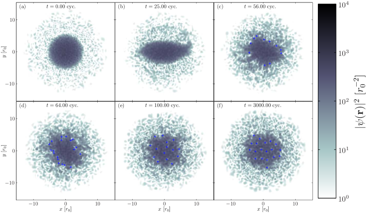
Figure 1: (Color online) Classical field density at representative times during the evolution. Shown are (a) initial condition: lab. frame ground state plus vacuum noise, (b) ejection of material during the dynamical instability, (c) nucleation of vortices at the interface between the condensate and the non-condensate material, (d) penetration of vortices into the condensate bulk, (e) non-equilibrium state with rapid vortex motion, and (f) equilibrium state. Vortices are indicated by $+$, and are shown only where the surrounding density of the fluid exceeds some threshold value. Parameters of the trajectory are given in the text.

Dynamical instability and formation of thermal cloud.— The initial state (Fig. 1(a)) quickly becomes elongated, with its long axis oscillating irregularly relative to the major axis of the trap. The quadrupole oscillations are dynamically unstable to the stirring perturbation Recati01 ; Sinha01 ; Parker06 , and since all the Bogoliubov modes of the condensate are effectively populated due to the representation of quantum noise in our simulation, some of the fluctuations grow exponentially. The effect is clearly seen in Fig. 1(b), where matter streams off the tips of the elliptically deformed condensate in the direction of the trap rotation. Material is then ejected more or less continuously, forming a ring about the condensate, with the latter oscillating in its motion and shape. The ring soon becomes turbulent and diffuse (Fig. 1(c)), losing coherence and forming a thermal cloud whose characterisation (Sec. V.1) is a central theme of this paper. In Sec. V.2.2 we show from an analysis of the angular momentum and density distribution that by $t=50$ cyc. the outer part of the cloud (beyond $r\approx 7r_{0}$) rotates as a normal fluid in rotational equilibrium with the drive.

Vortex nucleation.— After the thermal cloud has formed, surface oscillations of the condensate grow in magnitude (Fig. 1(d)), in accordance with the prediction of Williams et al., Williams2002a that such oscillations are unstable in the presence of a thermal cloud. These fluctuations form a transition region between the central condensate bulk, characterised by comparatively smooth density and phase distributions (see also Fig. 8(a)), and an outer region of thermally occupied highly energetic excitations. Long-lived vortices are nucleated in this transition region, and then begin to penetrate into the edges of the condensate region. Initially the vortices penetrate only small distances $r\approx r_{0}$ with rapid and irregular motion, and visibly lag the rotation of the drive. Penckwitt et al. Penckwitt02 have previously given a description of this vortex nucleation and penetration using a model in which a rotating thermal cloud was included phenomenologically.

Vortex array formation.— The nucleated vortices remain near the edge of the condensate for a considerable time before they begin to penetrate substantially into the condensate. Eventually vortices pass through the central region (by $t\approx 75$ cyc. in this simulation), with trajectories that are largely independent, except when two vortices closely approach each other note4 . The density of vortices within the central region gradually increases (Fig. 1(e)), and the vortices begin to form a rather disorderly assembly, which still lags behind the drive in its overall rotation about the trap axis. The erratic motion of individual vortices and their differential rotation with the respect to drive then gradually slow, and they become more localised, until by $t\approx 150$ cyc. they have formed into an array rotating at the same speed as the drive. This formation process can be interpreted as the damping of vortex motion by the mutual friction between them and the rotating thermal cloud Sonin87 ; Donnelly91 . Alternatively, we can interpret the motion of the vortices as the result of low energy excitations of the underlying vortex lattice state Sonin87 , which are gradually damped by their interaction with high energy excitations Fedichev98 ; Giorgini98 ; Pitaevskii97 . The coupling of the high-energy modes to the low-energy excitations of the lattice state, drives their distribution towards equilibrium Sagdeev88 ; Sinatra99 . The high energy modes comprising the thermal cloud equilibrate to a distribution with identifiable effective thermodynamic parameters (see Sec. V.1) on a relatively short timescale ($\sim 100$ cyc.). While the effective temperature remains approximately fixed, the effective chemical potential subsequently increases over a longer timescale ($\sim 3000$ cyc.), as the distribution is shaped by its interaction with the low energy excitations (including lattice excitations). By $t\approx 1000$ cyc. the vortex motion reaches its equilibrium level, and the equilibrium populations of lattice excitations at this temperature are such that the vortex distribution does not ‘crystallize’ into a rigid lattice. The damping of vortex motion is analysed quantitatively in Sec. V.4.

V Analysis

In this section we present the set of measurements we use to analyse the properties of the thermal cloud, and to identify the remaining condensate fraction. We begin by making a simple estimation of the energy and temperature the thermal cloud will acquire during the lattice formation. We obtain the chemical potential of the thermal cloud by using a self consistent fitting procedure for the atomic distribution function, which also provides a more accurate measure of the temperature. We characterise the rotational properties of different spatial regions of the system, which provides evidence that during the vortex nucleation stage, the central part behaves as a superfluid, while the outer cloud behaves as a classical gas, rotating like a rigid body.

The issue of condensate identification is a very important one, and is most commonly done in terms of spatial correlation functions, using ensemble averages of quantum mechanical operators Dalfovo99 ; Leggett01 . However, this is not well suited to the case of vortex lattice formation, due to varying vortex configurations within the ensemble, with correspondingly destructive effect on the spatial order of the system. In the classical field description of a finite temperature Bose gas, time averages are often substituted for ensemble averages, making use of the ergodic hypothesis Blakie05 . We show, in Sec. V.3 that temporal correlation functions can be used to characterise the local coherence of the field, and consequently determine the extent of the condensate mode and its eigenvalue.

Following the first appearance of an identifiable vortex array, there is a long period over which it slowly relaxes to an equilibrium state. In Sec. V.4 we measure the motional damping of the vortices and interpret it in terms of their interaction with the thermal component of the field Fedichev99 . Note that all results and figures in this section (Figs. 2-9) correspond to the simulation shown in Fig. 1.

V.1 Thermodynamic parameters

V.1.1 Analytic predictions

Since our system conserves both normalisation and energy in the rotating frame, some simple analytic predictions can be made about the development of the thermal component of the field, using the Thomas-Fermi (TF) approximation. In a frame rotating at angular velocity $\Omega$, the ground state is a vortex lattice which, neglecting the effect of the vortex cores, has Thomas-Fermi wavefunction

$$\psi_{\mathrm{TF}}^{\Omega}=\sqrt{\frac{\mu_{\Omega}-m\left(\omega_{r}^{2}-\Omega^{2}\right)r^{2}/2}{U_{\mathrm{2D}}}}\,\Theta\left(\mu_{\Omega}-m\left(\omega_{r}^{2}-\Omega^{2}\right)\frac{r^{2}}{2}\right),$$ (27)

where $\mu_{\Omega}$ is the chemical potential of the rotating frame solution. From Eq. (27) we obtain the number of particles $N_{\mathrm{TF}}^{\Omega}$ and energy $E_{\mathrm{TF}}^{\Omega}$ for the lattice state

$$N_{\mathrm{TF}}^{\Omega} = \frac{\pi\mu_{\Omega}^{2}}{U_{\mathrm{2D}}m\left(\omega_{r}^{2}-\Omega^{2}\right)},$$ (28)

$$E_{\mathrm{TF}}^{\Omega} = \frac{2}{3}\mu_{\Omega}N_{\mathrm{TF}}^{\Omega}.$$ (29)

The corresponding quantities for the vortex free inertial frame ground state are given by setting $\Omega=0$. We note that $\mu_{0}\equiv\mu_{\Omega=0}$ has the same value in both the stationary and rotating frames (since this solution is non-rotational). If we now compare a lattice state and a vortex free state, both fully condensed and with equal occupation, we see from Eq. (28) that the chemical potentials are related by

$$\mu_{\Omega}=\mu_{0}\sqrt{1-\Omega^{2}/\omega_{r}^{2}},$$ (30)

and hence from Eq. (29) that their rotating frame energies are related by

$$E_{\mathrm{TF}}^{\Omega}=E_{\mathrm{TF}}^{0}\sqrt{1-\Omega^{2}/\omega_{r}^{2}}.$$ (31)

The excess energy of the vortex free ground state over the lattice state of the same number of atoms,

$$\Delta E\equiv E_{\mathrm{TF}}^{0}-E_{\mathrm{TF}}^{\Omega}$$ (32)

can be significant, and for example is approximately $E_{\mathrm{TF}}^{0}/3$ for an angular velocity of $\Omega=0.75\omega_{r}$. Thus in our stirring scenario, the rotating equilibrium state reached at the end of the process must have less atoms and less energy than the initial vortex free state, and the excess energy and atoms constitute a thermal cloud note5 . The exact result for the excess energy of the classical field, obtained from the simulations, will depend upon the depletion of the condensate mode required to form the thermal cloud and the mutual interaction of the cloud with the condensate. For small thermal fractions this energy could be found by means of a calculation similar to that described in Ref. Sinatra00 . In the simplest approximation we assume the limit of a small thermal fraction, in which the energies of the condensate and thermal field are additive, with Eq. (32) approximating the excess energy the thermal field contains. We further assume that in equilibrium this energy will be classically equipartitioned over weakly interacting harmonic oscillators, in the spirit of the Bogoliubov approximation Lobo04 . The equilibrium temperature can thus be predicted by

$$T=\frac{\Delta E}{\mathcal{M}-1},$$ (33)

with $\mathcal{M}$ the condensate band multiplicity. For a given initial chemical potential we see therefore that the equilibrium temperature will be strongly dependent on the basis size. However, we shall see in Section VI, Eq. (30) provides a very good estimate of the final chemical potential reached by the field, which is essentially independent of cutoff.

V.1.2 Self-consistent fitting

We expect a procedure such as the self-consistent Hartree-Fock approximation described in Giorgini97 to provide a good estimate for both $\mu$ and $T$. However in order to avoid performing the iterative procedure presented in Giorgini97 we use a simpler approximation to this description, similar to that presented in Naraschewski98 , but with some necessary modifications. The TF approximation for the condensate mode employed in Naraschewski98 is a poor choice for the situation considered here, where the distribution of vortices is irregular and the density of vortices is low. Secondly a straightforward application of the model of Naraschewski98 to our system leads to divergences, as the semiclassical density distribution of non-condensed atoms becomes

$$n_{\mathrm{th}}(\mathbf{x})=\frac{1}{\lambda_{T}^{2}}g_{1}[e^{-(V_{\mathrm{eff}}(\mathbf{x})+2U_{\mathrm{2D}}(n_{\mathrm{c}}(\mathbf{x})+n_{\mathrm{th}}(\mathbf{x}))-\mu)/kT}],$$ (34)

with $V_{\mathrm{eff}}(\mathbf{x})=m(\omega_{r}^{2}-\Omega^{2})r^{2}/2$ the centrifugally dilated trapping potential in the rotating frame. The Bose function $g_{1}(z)$ diverges logarithmically Pathria96 as $z\rightarrow 1$, and thus the function $n_{\mathrm{th}}(\mathbf{x})$ diverges where $V_{\mathrm{eff}}(\mathbf{x})+2U_{\mathrm{2D}}(n_{\mathrm{c}}(\mathbf{x})+n_{\mathrm{th}}(\mathbf{x}))\rightarrow\mu$. Neglecting the mutual mean-field repulsion $2U_{\mathrm{2D}}n_{\mathrm{th}}(\mathbf{x})$ of non-condensed atoms (as in Naraschewski98 ) would therefore leave us with divergences in $n_{\mathrm{th}}(\mathbf{x})$. We are thus led to develop a fitting function for the non-condensed density $n_{\mathrm{th}}(\mathbf{x})$ only, and which therefore depends only on the total field density $n(\mathbf{x})$, which we measure from the classical field trajectory. The inclusion of the mean-field interaction between non-condensed atoms ensures that our function remains regular so long as the (fitted) chemical potential is less than the minimum value of the effective potential experienced by non-condensed atoms, a restriction which is not expected to constrain our fit in an unphysical manner. In this way we avoid both having to distinguish between condensed and non-condensed material in forming the mean-field potential, and having to iterate a self-consistent model to convergence. Our approach to determining $\mu$ and $T$ is as follows: The one-body Wigner function corresponding to a Bose field $\hat{\phi}(\mathbf{x})$ is defined

$$F(\mathbf{x},\mathbf{k})\equiv\int d\mathbf{y}\langle\hat{\phi}^{\dagger}(\mathbf{x}+\frac{\mathbf{y}}{2})\hat{\phi}(\mathbf{x}-\frac{\mathbf{y}}{2})\rangle e^{i\mathbf{k}\cdot\mathbf{y}},$$ (35)

and we assume here the non-condensate atoms in the condensate band to be well described by such a distribution, for which we further assume the approximate semiclassical form Castin01 ; Bagnato87

$$F(\mathbf{x},\mathbf{k})=\frac{1}{\exp[(\epsilon(\mathbf{x},\mathbf{k})-\mu)/T]-1}.$$ (36)

The semiclassical energy is

$$\epsilon(\mathbf{x},\mathbf{K})=\frac{\hbar^{2}\mathbf{K}^{2}}{2m}+V_{\mathrm{eff}}^{\mathrm{HF}}(\mathbf{x}),$$ (37)

with $\mathbf{K}$ the wave vector adjusted to the rotating frame Bradley08 , and the Hartree-Fock effective potential in the rotating frame is

$$V^{\mathrm{HF}}_{\mathrm{eff}}(\mathbf{x})=m(\omega_{r}^{2}-\Omega^{2})\frac{r^{2}}{2}+2U_{\mathrm{2D}}n(\mathbf{x}),$$ (38)

with the total field density the sum of the condensate and non-condensate (thermal) contributions $n(\mathbf{x})=n_{\mathrm{c}}(\mathbf{x})+n_{\mathrm{th}}(\mathbf{x})$. The factor of two here is the strength of the interaction between pairs of atoms when at least one of the pair is non-condensed Giorgini97 ; Naraschewski98 ; Castin01 . The classical field limit of Eq. (36) is obtained when $F(\mathbf{x},\mathbf{k})\gg 1$, which occurs when the parameter $(\epsilon(\mathbf{x},\mathbf{k})-\mu)/kT\ll 1$, and is given by its first order expansion in this parameter,

$$F_{\mathrm{c}}(\mathbf{x},\mathbf{k})=\frac{kT}{\epsilon(\mathbf{x},\mathbf{k})-\mu}.$$ (39)

It is important to note that although Eq. (39) is obtained here as the high occupation approximation to the bosonic distribution Eq. (36), (describing the classical equipartitioning of energy over phase-space cells of volume $1/h^{2}$), we expect it to apply to the equilibrium state of a weakly interacting classical field system even if the level occupations are $\lesssim 1$ Sinatra01 ; Lobo04 ; note6 . With the local rotating frame wave vector cutoff defined by $\hbar^{2}K_{\mathrm{R}}(\mathbf{x})^{2}/2m\equiv\max\{E_{\mathrm{R}}-V_{\mathrm{eff}}^{\mathrm{HF}}(\mathbf{x}),0\}$ Bradley08 , we find for the spatial distribution

$$n_{\mathrm{th}}^{\mathrm{fit}}(\mathbf{x},\mu,T) = \int_{0}^{K_{\mathrm{R}}(\mathbf{x})}\frac{K\;dK}{2\pi}F_{c}(\mathbf{x},K)$$

$$= \frac{1}{\lambda_{\mathrm{dB}}^{2}}\ln\left[\frac{E_{\mathrm{R}}-\mu}{V_{\mathrm{eff}}^{\mathrm{HF}}(\mathbf{x})-\mu}\right],$$

on $|\mathbf{x}|\leq r_{\mathrm{tp}}$, with $r_{\mathrm{tp}}=\sqrt{2E_{\mathrm{R}}/m(\omega_{r}^{2}-\Omega^{2})}$ the semiclassical turning point of the condensate band in the rotating frame, and $\lambda_{\mathrm{dB}}=\sqrt{2\pi\hbar^{2}/mk_{\mathrm{B}}T}$ the thermal de Broglie wavelength. This expression constitutes an appropriate fitting function for the non-condensed component of the classical field, which requires no explicit knowledge of the distribution of condensed atoms note7 . To obtain an estimate of $\mu$ and $T$ for our system, we sample the azimuthally averaged field density $\tilde{n}(r)\equiv\frac{1}{2\pi}\int_{0}^{2\pi}d\theta\;n(r,\theta)$ at $N_{t}$ equally spaced times over some period $t\in[t_{0}-T/2,t_{0}+T/2]$, and average over the sample times to obtain $\langle\tilde{n}(r)\rangle\equiv\sum_{i=1}^{N_{t}}\tilde{n}(r,t_{i})/N_{t}$. From this we construct the effective potential

$$\langle V_{\mathrm{HF}}^{\mathrm{eff}}(r)\rangle=m(\omega_{r}^{2}-\Omega^{2})r^{2}/2+2U_{\mathrm{2D}}\langle\tilde{n}(r)\rangle.$$ (41)

We then take as our fitting function

$$n_{\mathrm{th}}^{\mathrm{fit}}(r;\mu,T)=\frac{1}{\lambda_{\mathrm{dB}}^{2}}\ln\left[\frac{E_{\mathrm{R}}-\mu}{\langle V^{\mathrm{HF}}_{\mathrm{eff}}(r)\rangle-\mu}\right].$$ (42)

As our fitting function represents only the non-condensed component our field, we are obliged to avoid including significant condensate density in our fit to $\langle\tilde{n}(r)\rangle$. We therefore perform our fit of $n_{\mathrm{th}}^{\mathrm{fit}}(r)$ to $\langle\tilde{n}(r)\rangle$ over the domain $r\in[r_{-},r_{\mathrm{c}}]$, with $r_{-}$ the location of the occurrence of the minimum value of the effective potential, i.e., $\langle V^{\mathrm{HF}}_{\mathrm{eff}}(r_{-})\rangle=\min\{\langle V^{\mathrm{HF}}_{\mathrm{eff}}(r)\rangle\}$, which should approximately mark the peak of the non-condensed fraction and thus the boundary of the condensate Naraschewski98 . Within the central region $r<r_{-}$, the fitted density $n_{\mathrm{th}}^{\mathrm{fit}}(r)$ thus decays monotonically as $r\rightarrow 0$. An example of such a fit is shown in Fig. 2.

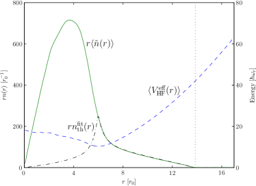
Figure 2: (Color online) Fitting procedure for the thermodynamic parameters. Shown are: the (time-averaged) radial density distribution times radius (solid line), the effective potential experienced by non-condensate atoms times radius (dashed line), and the fitted distribution of non-condensed atoms (dash-dot line). The dotted line indicates the classical turning point corresponding to energy cutoff $E_{\mathrm{R}}$. The data shown corresponds to the period $t=3000-3010$ cyc. (Fig. 1(f)).

After the initial strongly non-equilibrium dynamics following the dynamical instability (i.e. by $t\approx 400$ cyc.), the averaged field densities $\langle\tilde{n}(r)\rangle$ are fit well by the function given in Eq. (42), and we conclude that the higher energy components of the field have reached a quasistatic equilibrium. We follow thereafter the evolution of the temperature and chemical potential with time, which we present in Fig. 3. The temperature (Fig. 3(a)) appears to be essentially constant within the accuracy of the measurement procedure, while the chemical potential (Fig. 3(b)) shows a definite upward trend over the course of the field’s evolution. In Sec. V.3.2 we compare the chemical potential of the cloud determined from our fitting procedure, with the chemical potential of the condensate, which we extract by considering the temporal frequency components present in the field.

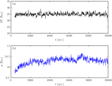
Figure 3: (Color online) Evolution of the effective (a) temperature and (b) chemical potential of the non-condensed atoms, as measured by the semiclassical fitting procedure.

V.2 Rotational parameters

A characteristic feature of superfluids is that they resist any attempt to impart a rotation to them, and they acquire angular momentum through the nucleation of vortices note8 , which endow the superfluid with quantized flow circulation (see e.g. Donnelly91 ). Thus while a classical fluid in equilibrium with a container rotating at angular velocity $\Omega$ satisfies the equality

$$\langle L_{z}\rangle=\Omega I_{\mathrm{c}},$$ (43)

where the classical moment of inertia is defined

$$I_{\mathrm{c}}\equiv m\langle r^{2}\rangle,$$ (44)

a superfluid in equilibrium with such a container will in general fail to do so. That is to say, the moment of inertia per particle

$$I\equiv\frac{\langle L_{z}\rangle}{N\Omega},$$ (45)

will not equal the classical value $I_{\mathrm{c}}/N$ in such a state. We note that for pure superfluids, such as a dilute Bose gas at $T=0$ (which is well described as a ground state of the GP equation), the steady state angular momentum is typically much less than the classical value determined by its mass distribution Zambelli01 . As the rotation frequency $\Omega$ of the GP state increases, the (areal) density of vortices increases Garcia-Ripoll01 ; Feder01 , and is given to leading order by the Feynman relation Donnelly91

$$\rho_{\mathrm{v}}^{\mathrm{c}}=\frac{m\Omega}{\pi\hbar},$$ (46)

with corrections arising due to the lattice inhomogeneity and the discrete nature of the vortex array Sheehy04 . As the rotation frequency and thus the vortex density increase, both the classical and quantum moments of inertia increase also, and the difference between the two moments vanishes in the limit of rapid rotations $\Omega\rightarrow\omega_{r}$ Feder01 .

V.2.1 Vortex density

To monitor the increase in vortex density during the system evolution, we count the vortices of positive rotation sense occurring within a circular counting region of radius equal to the TF radius of the initial state, $R_{\mathrm{TF}}=\sqrt{2\mu_{\mathrm{i}}/m\omega_{r}^{2}}$. Due to the rotational dilation of the condensate in the rotating frame this region lies within the central bulk of the condensate, and in this manner we attempt to avoid including in the count the short-lived vortices constantly created and annihilated at the condensate boundary. At equally spaced times over a period of 4 trap cycles about time $t_{i}$ we obtain the average number of vortices in the counting radius, $\langle n_{\mathrm{v}}(t_{i})\rangle$, and from this we determine the average vortex density in the counting region

$$\rho_{\mathrm{v}}(t_{i})=\frac{\langle n_{\mathrm{v}}(t_{i})\rangle}{\pi R_{\mathrm{TF}}^{2}}.$$ (47)

In Fig. 4(a) we plot Eq. (47) as a fraction of the prediction of Eq. (46). During the dynamical instability and initial nucleation of vortices the vortex densities measured in this manner are spuriously high, due to the counting of phase defects in the turbulent non-equilibrium fluid rather than long-lived vortices in the condensate bulk. After this initial period, i.e. from $t\approx 150$ cyc. onwards, we see a gradual increase in $\rho_{\mathrm{v}}$ as the condensate slowly relaxes and admits more vortices into its interior, and approaches rotational equilibrium with the trap. By $t\approx 6000$ cyc., the density appears to have essentially saturated at a level $\rho_{\mathrm{v}}\approx 0.85\rho_{\mathrm{v}}^{\mathrm{c}}$. Such a value seems reasonable for the rotation rate and condensate size considered here, which are such that inhomogeneity and discreteness effects will be significant Sheehy04 . Moreover, it seems plausible that the high degree of lattice excitation here increases the energetic cost of vortices above that assumed in the mean-field description of Sheehy04 .

V.2.2 Local rotational properties

In order to characterise the rotation of the outer cloud formed from ejected material as well as that of the central bulk of the field we measure localised expectation values, i.e. expectation values over a restricted spatial region. In this way we can compare the mass distribution and angular momentum of particular regions, in order to characterise the localised properties of the field. We define the expectation value of an operator $\mathcal{O}$ on spatial domain $\mathcal{D}$ by

$$\langle\mathcal{O}\rangle_{\mathcal{D}}=\int_{\mathcal{D}}d\mathbf{x}\;\psi^{*}\mathcal{O}\psi,$$ (48)

where the $\mathcal{D}$ will be either region $\mathcal{A}$ or $\mathcal{B}$ illustrated in Fig. 5. Focussing our attention on the outer annulus $\mathcal{B}$, we calculate the classical moment of inertia of material in the annulus

$$(I_{\mathrm{c}})_{\mathcal{B}}=m\langle r^{2}\rangle_{\mathcal{B}},$$ (49)

and the angular momentum of this material $\langle L_{z}\rangle_{\mathcal{B}}$. From measurements over the period $t=50-51$ cyc. we find that

$$\frac{\langle L_{z}\rangle_{\mathcal{B}}}{\Omega}=(I_{\mathrm{c}})_{\mathcal{B}},$$ (50)

to within 4%, indicating that the cloud in this region is rotating as a normal fluid in rotational equilibrium with the drive. Averaging samples of these expectation values over a period of a trap cycle, we find for the time averages $\{\langle\tilde{L_{z}}\rangle_{\mathcal{B}}/\Omega\}=1.025\{(\tilde{I_{\mathrm{c}}})_{\mathcal{B}}\}$.

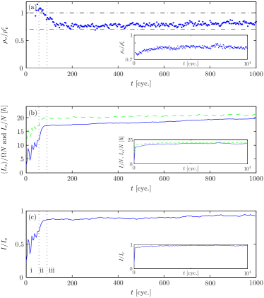
Figure 4: (Color online) Rotational response of the field. Shown are: (a) Vortex density, with dash-dot lines indicating $\rho_{\mathrm{v}}/\rho_{\mathrm{v}}^{\mathrm{c}}=0.7$ and $\rho_{\mathrm{v}}/\rho_{\mathrm{v}}^{\mathrm{c}}=1$ for reference, (b) classical (dashed line) and quantum moments of inertia, and (c) ratio of quantum and classical moments of inertia. Insets show the behaviour of the same quantities over a longer timescale. Note that the initial $L_{z}$ is finite due to the initial vacuum occupation. For reference dotted lines in (a-c) separate phases of the evolution discussed in the text.

Turning our attention to the central disc $\mathcal{A}$, we find that over the same period, $\{\langle\tilde{L_{z}}\rangle_{\mathcal{B}}\}/\Omega=0.080\{(I_{\mathrm{c}})_{\mathcal{B}}\}$. The central condensate bulk at this time thus remains approximately stable against vortex nucleation, but possesses some small angular momentum due to its shape oscillations, in contrast to the ejected material which has lost its superfluid character and has come to rotational equilibrium with the drive.

V.2.3 Global rotational properties

We consider now the rotational properties of the entire field, by evaluating expectation values as above over the full $xy$-plane, (i.e. in Eq. (48) we set $\mathcal{D}\rightarrow\mathbb{R}^{2}$). A measure of the field’s rotation is given by the angular momentum $L_{z}$. We plot the ratio $I/I_{\mathrm{c}}$ to characterise the response of the atomic field to the imposed rotation, as both the field’s angular momentum and its mass distribution change with time. In Fig. 4(b) we plot the evolution of these quantities as time evolves and in Fig. 4(c) we plot the evolution of their ratio.

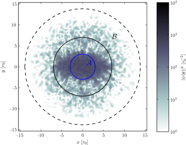
Figure 5: (Color online) Regions used for the evaluation of angular momenta and moments of inertia. Disc $\mathcal{A}$ lies entirely within the condensate, where the flow is (initially) irrotational. Annulus $\mathcal{B}$ (between the solid black line and the dashed line indicating the classical turning point of the condensate band) contains only non-condensed, normal fluid. The field density shown is that at $t=50$ cyc.

Comparing the evolution of these quantities and that of the field’s density distribution (c.f. Fig. 1), we identify three roughly distinct phases of the system evolution: (i) Excitation of unstable surface mode oscillations accompanied by permanent increase in angular momentum (c.f. Fig. 1(b)), (ii) further increase in angular momentum and $I/I_{\mathrm{c}}$ as vortices are nucleated into the condensate bulk (Fig. 1(c-e)), and (iii) gradual approach of the field to rotational equilibrium with the drive (Fig. 1(f)). Note that although the finite temperature equilibria here contain a significant normal fluid component, the quantum moment of inertia is still suppressed below the classical value due to the presence of the superfluid component.

V.3 Temporal analysis

V.3.1 Issues of condensate identification

A central concern in classical field simulations is the identification of the condensate mode and its occupation. In situations such as Norrie05 ; Norrie06a ; Norrie06b where the collisional dynamics dominate, and dynamics of interest occur on a short timescale, the condensate mode can be identified within a $U(1)$ symmetry-broken description as the coherent fraction of the field

$$\psi_{\mathrm{coh}}=\langle\hat{\psi}\rangle,$$ (51)

where the expectation value in the many-body state $\langle\cdots\rangle$ can be formally related to moments of the classical field Gardiner00 ; Gardiner02 .

However, on longer timescales the classical field is expected to evolve to a thermal distribution Sinatra02 ; Davis01 , and so we abandon the formal operator correspondences and examine the classical statistics of the trajectory ensemble directly. Furthermore, the chaotic nature of the system means that trajectories which are initially close in phase-space will, in general, diverge as it evolves. Thus even in an idealised situation in which distinct trajectories each contain a highly occupied mode undergoing coherent phase rotation, the phase of this mode at a particular time $t$ will vary between trajectories, and the identification of the condensate mode with the field operator mean yields a condensate fraction which decays spuriously as the neighbouring trajectories dephase. This is a natural consequence of the symmetry-broken condensate definition, and occurs even for small non-condensate fractions Lewenstein96 ; Castin98 , however the dephasing is intuitively expected to occur more rapidly in systems with a greater incoherent fraction.

However, global gauge symmetry breaking has no effect on the one body density matrix

$$\rho(\mathbf{x},\mathbf{x}^{\prime})\equiv\langle\hat{\psi}^{\dagger}(\mathbf{x})\hat{\psi}(\mathbf{x}^{\prime})\rangle,$$ (52)

or its classical field analogue Blakie05 . In a strongly thermal system, the ergodic hypothesis may be employed to approximate such an ensemble expectation value by a time average. Blakie and coworkers Blakie05 have used the Penrose-Onsager Penrose56 definition of the condensate mode (the single eigenmode of $\rho(\mathbf{x},\mathbf{x}^{\prime})$ with an occupation comparable to the total (mean) number of particles), to extract a condensate fraction from individual classical field trajectories, in equilibrium and quasi-equilibrium scenarios.

However, the Penrose-Onsager criterion is not appropriate for the current situation, which exhibits strongly non-equilibrium behaviour. As noted in Leggett01 , in such situations the Penrose-Onsager definition may fail to correctly describe the amount of condensation in the system. Further complexity is added by the presence of a non-trivial phase structure such as that of a condensate containing an array of vortices. Indeed even at $T=0$ in an axially symmetric trap, the rotating frame ground state is in general highly degenerate due to the spontaneous breaking of the rotational symmetry of the many-body Hamiltonian Seiringer08 . The corresponding one-body density matrix thus fails to describe a single highly occupied mode. While in our case the axial symmetry of the Hamiltonian is explicitly broken by the potential anisotropy $V_{\epsilon}(\mathbf{x})$, distinct configurations of vortices distinguish states of the system in a way which cannot be cancelled by global phase rotations. One-body density matrices calculated from either ensemble or ergodic time averages thus describe a non-simple or fragmented condensate state (see Leggett01 ). As this behaviour might be expected of the true one-body density matrix in such a situation, we regard this to be a lack in generality of the Penrose-Onsager criterion itself. A quantification of the condensate population or mode at a single time would therefore require a description in terms of higher order correlation functions.

V.3.2 Frequency distribution

Previous authors studying equilibrium systems have used known quasiparticle bases to extract frequency distributions from classical field simulations Davis02 ; Brewczyk04 . In a general non-equilibrium situation, with significant non-condensate populations, suitable modes can not be defined. We therefore use an alternative strategy, and extract information about the distribution of modes in the trap by analysing the frequencies present at particular points in position space. We define the power spectrum of the classical field $\psi$ at position $\mathbf{x}$ about time $t_{0}$

$$H(\mathbf{x},\omega;t_{0})=|\mathfrak{F}_{t_{0}}^{T}\{\psi(\mathbf{x},t)\}|^{2},$$ (53)

where $\mathfrak{F}_{t_{0}}^{T}\{f(t)\}$ denotes the Fourier coefficient

$$\mathfrak{F}_{t_{0}}^{T}\{f(t)\}\equiv\frac{1}{T}\int_{t_{0}-T/2}^{t_{0}+T/2}f(t)e^{-i\omega t}dt.$$ (54)

We choose a sampling period of 10 trap cycles so as to be long compared to the timescales characterising the phase evolution of the condensate ($\tau_{\mathrm{p}}\sim\hbar/\mu$), while being short compared to the that of the relaxation of the field ($\tau_{R}\sim 1000$ cyc.) Bradley08 , and choose the sampling interval so as to resolve all frequencies present due to the combined single particle and mean-field evolutions ($\hbar\omega_{\mathrm{max}}=E_{\mathrm{R}}+2\mu_{\mathrm{i}}$). We average this result over azimuthal angle $\theta_{j}$, to form $\tilde{H}(r,\omega,t_{0})$. In order to gauge the relative strength of the various frequency components at different radii within the classical region, we normalise the resulting data so that the total power at each radius $r_{j}$ is the same.

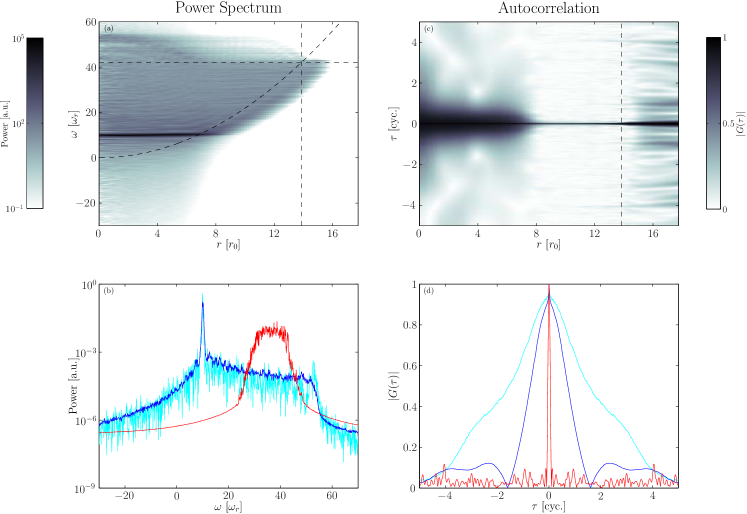
Figure 6: (Color online) (a) Azimuthally averaged power spectral density (PSD). Dashed lines indicate the cutoff energy, corresponding classical turning point and (centrifugally dilated) trapping potential. (b) PSD traces at particular radii. The black (blue) and dark grey (red) lines correspond to radii $r=3.1894r_{0}$ and $r=11.9575r_{0}$ respectively. The light grey (cyan) line corresponds to the smallest measured radius. (c) Autocorrelation function (absolute value) obtained from the power spectrum. The dashed line indicates the classical turning point of the condensate band. (d) Autocorrelation magnitude at radii corresponding to Fig. 6(b). Data corresponds to the period $t=9900-9910$ cyc.

In Fig. 6(a), we plot the result of such a calculation over the time interval $t=9900-9910$ trap cycles. For comparison we have overlaid the centrifugally dilated potential $V_{c}(r)=m(\omega_{r}^{2}-\Omega^{2})r^{2}/2$ that would be seen by a classical particle in the rotating frame, the cutoff frequency $\omega_{\mathrm{R}}=E_{\mathrm{R}}/\hbar$, and the semiclassical turning point $r_{\mathrm{tp}}$. Several notable features are present. At small radii we see a prominent peak in the power spectrum at $\omega\approx 10\omega_{r}$, which we interpret as the coherent phase rotation frequency of the underlying condensate mode, i.e., the condensate eigenvalue $\mu_{\mathrm{c}}/\hbar$. In Fig. 6(b) where the power spectrum is plotted at 3 particular radii, the peak in the spectrum obtained close to the trap centre (light gray/cyan line) can be seen clearly. In addition we see that frequencies above and below this are present, and we identify these as due to the thermal occupation of the quasiparticle ‘particle’ and ‘hole’ modes respectively. At this same radial value ($r=0.0661r_{0}$) a secondary peak is visible at $\omega\approx 52\omega_{r}=(\mu_{\mathrm{c}}+E_{\mathrm{R}})/\hbar$. An examination of the data reveals that a smaller peak is also present at $\omega\approx-32\omega_{r}=(\mu_{\mathrm{c}}-E_{\mathrm{R}})/\hbar$. This is an artifact of the projected method which occurs as follows: The $\mathcal{M}$ Bogoliubov modes which diagonalize the Bogoliubov Hamiltonian in the condensate band in the presence of a stationary condensate mode (GP eigensolution) can be considered as variational approximations to the lowest-lying ‘true’ Bogoliubov modes (obtained as the cutoff $E_{\mathrm{R}}\rightarrow\infty$). The highest energy modes in the restricted quasiparticle basis are poor representations of the true modes, and, to maintain orthogonality of the set, are spuriously localised to the trap centre, and therefore have spuriously high energies $\epsilon_{k}+\mu_{\mathrm{c}}\approx E_{\mathrm{R}}+\mu_{\mathrm{c}}$ due to the large mean-field interaction there. Therefore, assuming this behaviour of excitations to hold in a finite temperature equilibrium of the classical field, a peak is expected to occur at these frequencies at the trap centre, where the density of these modes is comparatively large. However the population contained in the peak observed here is $\sim 0.5\%$ of the total thermal population and as such we do not expect it to qualitatively affect the relaxation process note9 . The black (blue) line in Fig. 6(b) indicates the power spectrum at a larger radius where the peak is slightly less prominent. At larger radii still ($r\gtrsim 9r_{0}$) the energy distribution returns to approximately that of the non-interacting gas. Frequencies persist into the classically excluded region as a result of the familiar evanescent decay of energy eigenmodes into the potential wall. The effect of the mean-field interaction on the energy spectrum at this large radii, as can be seen in the dark gray (red) line in Fig. 6(b), is much less dramatic (e.g., only frequencies $\omega>\mu_{\mathrm{c}}/\hbar$ are present), and the population of frequencies is only significant up to a small increment above the cutoff energy, which we interpret as the mean-field shift of the highest energy single-particle modes. We measure this shift to be $\approx 2.5\%$, indicating that the cutoff we have chosen is sufficiently high to contain all modes significantly modified by the condensate’s presence (see Sec. II.2).

In order to follow the relaxation of the condensate, we measure the frequency $\omega_{\mathrm{p}}$ of maximum occupation in the power spectra, for power spectra evaluated over various periods. Away from equilibrium this frequency does not necessarily correspond to the condensate eigenvalue, as many strong collective excitations are present. Nevertheless it provides a measure of the energy of condensate atoms, and we interpret it as representing an effective condensate chemical potential $\mu_{\mathrm{p}}=\hbar\omega_{\mathrm{p}}$. In Fig. 7 we plot the condensate chemical potential obtained in this way and also the chemical potential of the thermal cloud obtained using our fitting procedure (Section V.1.2) for comparison. We see that the condensate chemical potential reduces with time, as interactions with thermally occupied modes damp its excitations. By $t\approx 4000$ cyc., the two chemical potentials appear to have reached diffusive equilibrium, to the accuracy of our fitting procedure for $\mu$ and $T$.

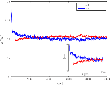
Figure 7: (Color online) Effective chemical potential of the condensate and thermal cloud. The data displayed is obtained from 10 trap cycle long samples spaced at 100 trap cycle intervals. Inset: Data with samples spaced at 10 trap cycle intervals over the initial decay (rise) of $\mu_{\mathrm{p}}$ ($\mu_{\mathrm{th}}$).

V.3.3 Temporal coherence and condensate identification

The power spectrum discussed above shows clearly that a condensate is present within the classical field, presenting as its signature the presence of a single highly occupied frequency, broadened by its interactions with the other modes in the system. The presence of this narrow frequency spike is indicative of the temporal coherence of this condensate mode, and we will use the local autocorrelation function

$$G(\mathbf{x},\tau;t_{0})=[\mathfrak{F}_{t_{0}}^{T}]^{-1}\{H(\mathbf{x},\omega;t_{0})\},$$ (55)

of the field at point $\mathbf{x}$, at lag $\tau$ relative to the time $t_{0}$ to quantify the local temporal coherence of the field. To do so we employ the Wiener-Khinchin theorem Press92 to evaluate the local autocorrelation function.

In practice we take the discrete Fourier transform of $\tilde{H}(r_{k},\omega;t_{0})$ to obtain the azimuthally averaged autocorrelation $\tilde{G}(r_{k},\tau;t_{0})$, and normalise it so that $|\tilde{G}(r_{i},\tau=0,t_{0})|=1$ for all radii $r_{i}$. We will use the modulus $|\cdots|$ to characterise the temporal coherence of the classical field, as a function of position, and take the timescale for its decay to represent the timescale over which the field remains temporally coherent at radius $r_{k}$, near time $t_{0}$. Illustrative results are shown in Figs. 6(c) and (d).

At the centre of the trap (light gray/cyan line in Fig. 6(d)), the peak of the autocorrelation function is broad and decays monotonically with increasing $|\tau|$. At larger radii ($r\approx 2r_{0}-5r_{0}$), this peak possesses a nontrivial structure (black/blue line), with $|\tilde{G}|$ vanishing and then increasing again as $\tau$ varies. Analyzing the trajectories of vortices during the sampling period we conclude that this structure is due to the passage of vortices through these radii. We identify the width of the central peak (Fig. 6(d)) at a radius $r_{i}$ as (twice) the correlation time of the classical field at this radius. At the trap centre, the correlation time $t_{\mathrm{c}}\approx 2.2$ cyc., indicating that despite the presence of highly energetic thermal excitations and mode mixing in the central region, the temporal coherence of the condensate mode is significant. We note also that a small ridge appears in $|\tilde{G}(\tau)|$ for $\tau$ close to zero, and interpret this as representing the correlations of the thermal component of the field (see also Bezett08 ).

The width of the broad envelope (Fig. 6(d)) decreases with increasing radius around $r=8r_{0}$, where the strong peak in the power spectrum also reduces. Past this point the peak becomes much narrower (dark grey/red line in Fig. 6(d)); the short correlation time of the outer cloud reflecting the broad range of energies characteristic of the thermally occupied excitations. Beyond the classical turning point, the evanescent nature of the basis modes yields a spurious amount of temporal coherence and this manifests as an increasing correlation time past this point (a similar phenomenon was observed for spatial correlations in Bezett08 ).

While the interpretation of the correlation time we calculate in this manner is complicated by the non-monotonic decay of $|\tilde{G}(\tau)|$ with increasing $|\tau|$, it nevertheless allows us to distinguish turbulent behaviour from thermal behaviour. For example, in Fig. 8(a) and (b) we plot the phase profile of condensate band at time $t=100$ cyc, and the corresponding correlation time respectively. The correlation time maintains a near-constant value of $t_{\mathrm{c}}\approx 1.1$ cyc. as $r$ increases until $r\approx r_{0}$, where the first vortex (phase singularity in Fig. 8(a)) occurs. At this point the correlation time begins to decay steeply with increasing $r$. Throughout the region $r<r_{\mathrm{tp}}$ the phase structure is complicated, however we see that the correlation time of the central region is at least of order $t_{\mathrm{c}}\sim 0.5$ trap cycles, indicating that despite the turbulent nature of the field here, interactions serve to maintain its coherence, and we identify the behaviour here as superfluid turbulence Barenghi01 , in contrast to the outer region ($r\gtrsim 6r_{0}$), which has a very short correlation time and thus appears to be truly thermal material. This is in contrast to the interpretation presented by the authors of Parker05a ; Parker06b , who considered the turbulence developed during the stirring process to be purely superfluidic (i.e., zero temperature) in nature.

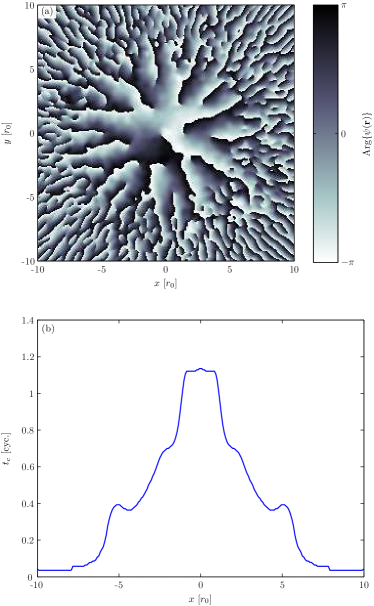
Figure 8: (Color online) Plots of (a) the condensate band phase and (b) the corresponding correlation time as a function of radius, near time $t=100$ cyc.

V.4 Vortex motion

As noted in Sec. IV, the motion of vortices (as viewed in the rotating frame) is initially very rapid, and slows as time goes on. In order to quantify this motion and its slowing with time, we track vortex trajectories, monitoring the coordinates of all vortices within a circular region of radius equal to the Thomas-Fermi radius of the initial lab-frame condensate. Due to the rotational dilation of the vortex-containing condensate, this region always lies within the central bulk of the condensate, as defined by the temporal analysis described above. In general, vortices enter and leave this counting region as time progresses. We are interested in the motion of vortices which persist in the counting region and can therefore be considered to exist in the condensate, rather than those which occur in the violently evolving condensate periphery. We therefore discard the trajectories of all vortices which do not remain in the region for at least half the counting period of $T_{\mathrm{v}}=10$ trap cycles about time $t_{i}$.

The motion of the remaining vortices is erratic on a length scale of order of the healing length, which is the manifestation of thermal core-filling in the classical field model. As this motion occurs on a short timescale, we interpret it as the signature of high-energy excitations of the vortices. Our interest however is in the low energy component of vortex motion, which undergoes damping as the field relaxes to equilibrium. We therefore apply a Gaussian frequency filter centred on $\omega=0$ to the trajectory components $\{x(t),y(t)\}$ to remove their highest temporal frequency components. We choose the width of this filter to be $\sigma_{\omega}\sim 0.6\omega_{r}$, and so the frequency components preserved in the trajectories correspond to low energy excitations ($\omega\sim\omega_{r}$). From the $N_{t}$ coordinate pairs $(x_{k},y_{k})$ of the $j^{\mathrm{th}}$ filtered vortex trajectory we extract the mean speed along the trajectory arc,

$$v_{j}(t_{i})=\frac{1}{T_{\mathrm{v}}}\int ds\approx\frac{1}{T_{\mathrm{v}}}\sum_{i=1}^{N_{t}-1}\sqrt{(x_{i}-x_{i-1})^{2}+(y_{i}-y_{i-1})^{2}}.$$ (56)

We then average this quantity over the vortices included in the count, to find the mean speed per vortex $\overline{v}(t_{i})=\sum_{j=1}^{N_{\mathrm{v}}}v_{j}(t_{i})/N_{\mathrm{v}}$. In Fig. 9 we plot this quantity as a function of time. We note firstly that the mean vortex speed decays dramatically during the initial measuring period $t\approx 70-150$ cyc., as vortices enter the condensate with high velocities (with a substantial component opposing the trap rotation, as observed in the rotating frame), and their motion is damped heavily by their interaction with one another and with the thermal component. Subsequent to this, a secondary, slower damping is observed over the period $t\approx 150-1100$ cyc., after which the vortex motion seems to have reached a lower limit set by thermal excitations. During this period the condensate contains nearly the number of vortices it contains in equilibrium, and we interpret the damping during this period as the damping of low energy lattice excitations due to their interaction with thermally occupied, high energy modes. Taking the log of the speed data (Fig. 9 inset), we see that the decay during this period is approximately exponential, and performing a linear fit to the data over this period we extract a damping rate $\gamma\approx 6.3\times 10^{-4}$ $(\mathrm{cyc.})^{-1}$.

We note that the final distribution of vortices is disordered, with the vortices failing to become localised in a regular lattice. This result is consistent both with the considerations of Sec. V.1 and with pure GPE studies of stirring in 2D performed by Feder et al. Feder01a , and Lundh et al. Lundh03 . The results presented here (and those of Lobo04 ) suggest that the turbulent states observed in Feder01a ; Lundh03 are in fact finite temperature ones beyond the validity of the GP model employed in those calculations. By contrast, the calculations of Parker et al. Parker06b ; Parker05a produced fully crystallized vortex lattices in 2D, indicating that additional damping mechanisms were available to the system in their simulations. It is possible that these are attributable to the spatial differencing technique Parker_PhD ; note13 used in those calculations, which is known to be less accurate note14 than the methods used in the present work, and Refs. Feder01a ; Lundh03 .

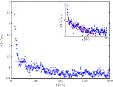
Figure 9: (Color online) Mean vortex velocity measured from the classical field trajectory, revealing the rapid slowing of vortices during the initial stage of nucleation ($t\approx 0-120$ cyc.), and more gradual damping of the remaining collective excitations ($t\approx 100-1000$ cyc.). Inset: Logarithm of the mean vortex velocity (scaled by the minimum velocity measured $\bar{v}_{\mathrm{min}}$), and linear least-squares fit to the data over the damping period.

VI Dependence on simulation parameters

We compare now the behaviour of stirred condensates for different condensate sizes, i.e., for different values of the initial chemical potential $\mu_{\mathrm{i}}$. The field density and thus the nonlinear effects of mean-field interaction increase as the chemical potential is increased, and larger condensates in rotational equilibrium will also contain larger numbers of vortices. In Sec. VI.1 we assess the effect of varying initial chemical potential on our classical field solutions.

It is also important in performing classical field calculations such as those presented here to consider the effect of the cutoff height on the results of simulations. In Appendix IX we compare results for simulations with fixed initial chemical potential but varying cutoff heights, and quantify the effect of this purely technical parameter on the physical predictions of our model.

VI.1 Chemical potential

The initial chemical potential impacts upon the system evolution both qualitatively, affecting the density profile of the condensate mode and thus the nature of the dynamical instability leading to vortex nucleation, and quantitatively, determining the equilibrium parameters of the stationary state of the classical field. The characteristics of the vortex array and dynamics of the vortices are also strongly dependent on the chemical potential. We consider these three aspects in turn.

VI.1.1 Effect on dynamical instability

The chemical potential determines the strength of the mean-field repulsion influencing the condensate’s shape. As the chemical potential becomes large, the condensate mode approaches that described by the Thomas-Fermi approximation, whereas for smaller chemical potentials, the kinetic energy of the condensate becomes important, and the condensate boundary broadens. Consequently the visual distinction between the condensate mode and its incoherent excitations becomes less clear as the chemical potential is reduced. This affects the early evolution of the system and the onset of the dynamical instability in a pronounced manner. For the largest chemical potentials considered ($\mu\approx 17-20\hbar\omega_{r}$), the collective (quadrupole) excitations and their breakdown are clearly visible against a background of incoherent noise resulting from the initial vacuum occupation. For smaller chemical potentials, while quadrupole oscillations are still visible and the outer cloud becomes visibly more dense as time proceeds, indicating that material is indeed lost from the condensate, any ejection of material from the condensate is obscured by the blurred condensate boundary. Persistent ‘ghost’ vortices can be seen forming in the incoherent region about the condensate periphery very early in the evolution ($t\approx 20$ cyc. for $\mu_{\mathrm{i}}=4\hbar\omega_{r}$). In Fig. 10 we plot the evolution of the field angular momentum per atom for three different initial chemical potentials. The most obvious feature is that larger condensates support more angular momentum per atom, due to increased mean-field effects. The evolution of the field angular momentum for the smallest condensate considered ($\mu_{\mathrm{i}}=4\hbar\omega_{r}$) reveals the onset of irreversible coupling of angular momentum into the field at $t\approx 130$ cyc. Inspection of the field density evolution shows that vortices begin to be nucleated into the central region of the field at about this time. We therefore conclude that despite the absence of visible break-up of the condensate, the unstable quadrupole oscillations still serve to produce the thermal component required to allow vortices to enter the central condensate region note10 .

Figure 10: (Color online) Evolution of the field angular momentum for various initial chemical potentials.

VI.1.2 Thermodynamic parameters

As described in Section V.1, a simple analysis based on energetic considerations allows us to predict the equilibrium temperatures and chemical potentials of our classical field simulations, and the dependence of these parameters on the initial chemical potential and the condensate band multiplicity of our simulations. In Fig. 11 we plot these analytic predictions alongside the values obtained using the fitting procedure of Section V.1. The dotted line shows the estimated chemical potential of the (idealised) norm conserving, rotating frame condensate mode, $\mu_{\Omega}=\mu_{\mathrm{i}}\sqrt{1-\Omega^{2}/\omega_{r}^{2}}$, while the dash-dot line indicates the estimated equilibrium temperature given by Eq. (33). We note that despite its approximate (TF-limit) and asymptotic (zero thermal fraction) nature, the analytical estimate for $\mu$ is a reasonable prediction of the measured values. The measured value of $\mu$ is slightly higher than the TF prediction, and this discrepancy appears to increase with increasing $\mu_{\mathrm{i}}$, while the measured temperature appears consistently smaller than the analytical prediction at small $\mu_{\mathrm{i}}$, and exceeds it as the initial chemical potential is increased. However, the agreement seems very reasonable given the simplicity of the arguments presented in Section V.1, which neglect both the kinetic energy of vortices (TF approximation), the depletion of the condensate population and all other effects beyond a linear (Bogoliubov) description. We therefore conclude that our simple analysis captures the essential physics determining the thermodynamic parameters of the equilibrium. That is to say, the temperature is determined by the necessity of the system to redistribute the excess energy of the initial state (as viewed in the rotating frame), and that no additional heating of the system is required for the system to migrate to a state containing vortices.

Figure 11: (Color online) Equilibrium temperatures and chemical potentials reached as a function of initial chemical potential, as determined by the fitting procedure. Dotted and dash-dot lines indicate the predictions of Eq. (30) and Eq. (33) respectively. Numbers indicate times at which the measurements were made (thousands of trap cycles) in cases where numerical results were constrained by time. Points without numbers were measured at $10^{4}$ cyc.

VI.1.3 Vortex array structure

Perhaps the most striking difference between vortex arrays in simulations of differing condensate populations is the number of vortices present. As noted in Sec. V.2, the density of vortices is largely determined by the rotation rate of the condensate and is given to leading order by Eq. (46), and (within the TF approximation) the total number of vortices in an equilibrium condensate is approximately proportional to the chemical potential $\mu$.

The stability of a vortex array in equilibrium is determined by the competition between hydrodynamic and energetic considerations Donnelly91 which favour the crystallization of a rigid lattice, and the perturbing effect of thermal fluctuations in the atomic field. Close to zero temperature these fluctuations are interpreted as the thermal occupation of Bogoliubov excitations of the underlying vortex lattice state. As the temperature of a vortex lattice state is increased it eventually undergoes a transition to a disordered state Bradley08 as the long-range order of the lattice is degraded by thermal fluctuations.

After a long time period, $t\sim 10^{4}$ trap cycles, all our simulated fields appear to describe states on the disordered side of this transition. All our solutions have vortices migrating within the condensate bulk, and leaving and entering through the condensate periphery. In the the smallest condensates, with the smallest vortex counts (i.e. $\mu=(4,5,6)\hbar\omega_{r}$ with counts $N_{\mathrm{v}}\approx(4,5,6)$), the vortex array is small enough that quasi-regular configurations of vortices may occur, in which the vortex positions appear to fluctuate about approximate equilibrium positions on a triangular (or square) lattice. Such configurations may persist for as long as $\sim 10$ trap cycles, but ultimately breakdown and give way to new configurations as vortices cycle in and out of the central, high density region of the field. We interpret this cycling behaviour as the classical field ‘sampling’ different configurations during its ergodic evolution note11 .

Larger vortex arrays appear to be prohibited from forming regular structures over scales larger than nearest-neighbour inter-vortex separations (the scale of the apparent order in the smaller condensates). As noted in Sec. V.1, the equilibrium temperature attained by our simulated atomic fields increases linearly with the initial chemical potential, and so it seems unlikely that this behaviour would abate when the condensate size is increased further. Fig. 12(a-c) we plot the coordinate space densities of vortex arrays of differing sizes, corresponding to differing initial chemical potentials. Because of their small size compared to the extent of the condensate, vortex cores are difficult to experimentally image in situ, and so their presence is typically detected after free expansion of the atom cloud Lundh98 by absorptive imaging techniques. For condensates in the TF regime the expansion is well described by a simple scaling of the position-space density Kagan96 ; Castin96 (though the vortex core radius grows in somewhat greater proportion Lundh98 ). The Beer-Lambert law Robinson96 for the absorption of an optical probe, and the assumption of a ground-state (Gaussian) profile in $z$ yields for the transmitted intensity of the probe

$$I(x,y)=I_{0}e^{-\gamma|\psi(x,y)|^{2}},$$ (57)

with $I_{0}$ the input probe intensity and $\gamma$ a constant which depends, in general, on the absorptance of the atomic medium. In Figs. 12(d-f) we plot simulated intensity profiles obtained using Eq. (57), where we have in each case simply set $\gamma=2/\{|\psi|^{2}\}_{\mathrm{max}}$, with $\{|\psi|^{2}\}_{\mathrm{max}}$ the peak value of the density occurring in the distribution, so as to best represent the significant features. This process accentuates both the disparity in density between the condensate and the outer thermal cloud, and the density fluctuations in the central condensate region, in contrast to the logarithmic plots (Figs. 12(a-c)) which suppress them. The images show the thermally-distorted vortex array structure that might be measured in an experiment. The fact that the formation of rigid vortex lattices here is inhibited by thermal fluctuations, while ordered lattices have been formed experimentally at comparatively high temperatures Abo-Shaeer02 ; Madison00 , suggests that this inhibition of lattice order may be a manifestation of the well-known susceptibility of two-dimensional system to long-wavelength fluctuations Posazhennikova06 . Indeed (to our knowledge), no investigations of the effect of rotation on the BEC and BKT phases of Bose gases in quasi-2D trapping geometries have been performed to date note12 .

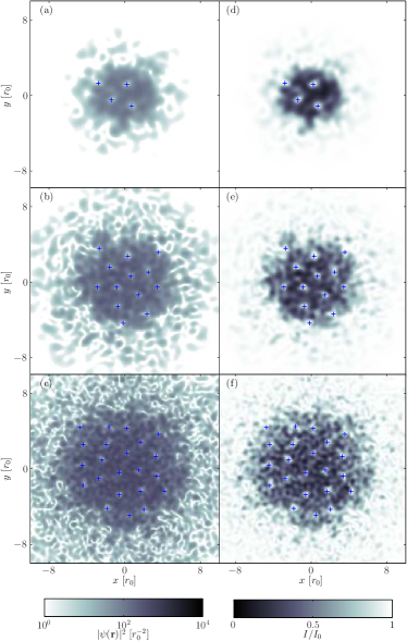
Figure 12: (Color online) (a-c) Coordinate space densities of the classical fields with initial chemical potentials $\mu_{\mathrm{i}}=5,10,18\hbar\omega_{r}$ at times $t=9900,9900,8800$ cyc. respectively. (d-f) Simulated absorption images generated from the same densities.

VI.1.4 Damping of vortex motion

While the vortex motion as measured by the mean velocity defined in Sec. V.4 exhibits the same overall damping behaviour in all our simulations, the damping appears to be generally non-exponential and quite sensitive to the initial noise conditions. We have observed additional features (e.g. transient and oscillatory behaviours superposed with the damping) peculiar to each trajectory. It is therefore difficult to unambiguously quantify the rates of motional damping in order to compare the dependence on initial chemical potential, without generating ensemble data for each parameter set, which would be a very heavy task numerically. We therefore plot in Fig. 13(a) only the behaviour of three particular trajectories, which indicate at a qualitative level that the vortex motion in the smaller condensates damps to equilibrium more quickly. We note however that the level of vortex motion that each trajectory damps to shows a clear dependence on the initial chemical potential. In Fig. 13(b) we plot the mean velocity of vortices over the period $t=1900-2000$ cyc., at which point the motion in each simulation appears to have essentially relaxed to its equilibrium level. The mean velocity so measured clearly increases with chemical potential. After comparing the results for varying cutoff at fixed initial chemical potential (not shown) we conclude that this is likely due to the increase in equilibrium temperature with increasing initial condensate size.

Figure 13: (Color online) (a) Vortex motional damping for 3 representative choices of initial chemical potential $\mu_{\mathrm{i}}$. (b) Mean vortex motion (averaged over the period $t=1900-2000$ cyc. as a function of initial chemical potential $\mu_{\mathrm{i}}$.

VII Conclusions

We have carried out the first strictly Hamiltonian simulations of vortex nucleation in stirred Bose-Einstein condensates. Our approach is free from grid method artifacts such as aliasing and spurious damping at high momenta, enabling a controlled study of the thermalization and vortex nucleation within an explicitly Hamiltonian classical field theory.

Vacuum symmetry breaking.—The importance of symmetry breaking has been highlighted in previous works Penckwitt02 ; Parker05a ; Parker06b . Sampling of initial vacuum noise provides an irreducible mechanism for breaking the twofold rotational symmetry of the classical field solution.

Thermalization.—Resonant excitation of the quadrupole instability evolves the system from a zero temperature initial state through a dynamical thermalization phase in which a rotating thermal cloud forms. Subsequent vortex nucleation in the remaining condensate shows that the cloud provides the requisite dissipation to evolve the condensate subsystem toward a new quasi-equilibrium state in the rotating frame. This picture is consistent both with energetic constraints of a time independent rotating frame Hamiltonian and with previous treatments based on introducing dissipation into the GP equation Tsubota02a ; Penckwitt02 .

Identifying the thermal cloud.— We have quantified the heating caused by dynamical instability through a range of measures. Spectral analysis of ergodic classical field evolution has been used to identify the condensate chemical potential, and thermal cloud properties were extracted using a semiclassical fit at high energies. While the chemical potentials of the condensate and emerging thermal cloud are slower to equilibrate, the moments of inertia, temperature, and angular momentum of the classical field are rapidly transformed by the instability to those of a rotating, heated Bose gas.

Frustrated crystallization.—Vortices are seen to nucleate and enter the bulk of the condensate but a regular Abrikosov lattice does not form. Instead the vortices distribute throughout the condensate in spatially disordered vortex liquid state, consistent with substantial thermal excitation of an underlying regular vortex lattice state. In this respect our results are consistent with previous 2D GPE treatments of similar stirring configurations.

We conclude that vortex nucleation by stirring is a finite temperature effect, which arises from dynamical thermalization when initiated from a zero temperature BEC. While we observe vortex nucleation in 2D, the asymptotic absence of lattice rigidity suggests that the temperature attained in accommodating the excess (rotating frame) energy of the initial state is such that vortex lattice crystallization is inhibited in this minimal, conserving stirring scenario in 2D.

VIII Calculation of the trap anisotropy

In this appendix we outline our numerical method for calculating the dimensionless perturbing potential $V_{\epsilon}(\bar{r})=-\frac{\epsilon}{2}\bar{r}^{2}\cos(2\theta)$. To calculate this term we follow Bradley08 in exploiting the properties of the Laguerre-Gaussian basis modes to evaluate this perturbation exactly using a Gauss-Laguerre quadrature rule. Changing variables Eq. (26) becomes

$$H_{nl}(\psi) = -\frac{\epsilon}{4\pi}\int_{0}^{2\pi}d\theta e^{-il\theta}\cos(2\theta)$$

$$\times\int_{0}^{\infty}dxx\Phi_{nl}(x)\psi(\sqrt{x},\theta)\pi,$$

where $\Phi_{nl}(x)=Y_{nl}(\sqrt{x},\theta)e^{-il\theta}$. The integral to evaluate is therefore of form

$$H_{nl}(\psi)=\frac{1}{4\pi}\int_{0}^{2\pi}d\theta e^{-il\theta}\cos(2\theta)\int_{0}^{\infty}dxe^{-x}Q(x,\theta),$$ (59)

where $Q(x,\theta)$ is a polynomial in $x$ and $e^{i\theta}$ of order determined by the cutoff. The order of $e^{i\theta}$ in $\psi(\mathbf{x})$ is constrained by Eq. (23) to be $-\overline{l}_{-}\equiv-l_{-}(0)\leq l\leq l_{+}(0)\equiv\overline{l}_{+}$, where $l_{\pm}(n)=[(\overline{N}-2n)/(1\mp\Omega)]$, with $[...]$ denoting the floor function. Choosing the $\theta$ grid so as to accurately compute all integrals $\frac{1}{2\pi}\int_{0}^{2\pi}d\theta e^{-iq\theta}$, where $q$ is an integer in the range $-(\overline{l}_{-}+\overline{l}_{+}+2)\leq q\leq(\overline{l}_{-}+\overline{l}_{+}+2)$, the integral can be carried out exactly for the condensate band by discretizing $\theta$ as $\theta_{j}=j\Delta\theta=j2\pi/N_{\theta}$, for $j=0,1,\cdots,N_{\theta}-1$, where $N_{\theta}=\overline{l}_{-}+\overline{l}_{+}+3$, to give

$$\int_{0}^{2\pi}d\theta e^{-il\theta}\cos(2\theta)=\frac{2\pi}{N_{\theta}}\sum_{j=0}^{N_{\theta}-1}e^{-i2\pi jl/N_{\theta}}\cos(2\theta_{j})Q(x,\theta_{j}).$$ (60)

The $x$-integral is computed by noting that the polynomial part of the $x$-integrand when the angular integral is nonzero is of maximum order $[\overline{N}/(1-\Omega)]\equiv\overline{l}_{+}$, which can be computed exactly using a Gauss-Laguerre quadrature rule of order $N_{x}\equiv[\overline{l}_{+}/2]+1$. The radial integral in Eq. (59) is

$$\int_{0}^{\infty}dxQ(x,\theta)e^{-x}=\sum_{k=1}^{N_{x}}w_{k}Q(x_{k},\theta),$$ (61)

where the $x_{k}$ are the roots of $L_{N_{x}}(x)$ and the weights $w_{k}$ are known constants Cohen73 . We can thus write Eq. (VIII) as

$$H_{nl}(\psi) = -\frac{\epsilon}{2}\sum_{k=1}^{N_{x}}\tilde{w_{k}}\Phi_{nl}(x_{k})\frac{1}{N_{\theta}}\sum_{j=0}^{N_{\theta}-1}e^{-i2\pi jl/N_{\theta}}$$

$$\times\cos(4\pi jl/N_{\theta})\psi(\sqrt{x_{k}},\theta_{j}),$$

where the effective weights $\tilde{w}_{k}=\pi w_{k}x_{k}$. Once the modes are precomputed at the Gauss points

$$P_{kn}^{|l|}=\Phi_{n|l|}(x_{k}),$$ (63)

the mixed quadrature rule for calculating the perturbation due to the trap anisotropy is:

1. Compute the radial transform

   $$\chi_{kl}=\sum_{n=0}^{[\overline{N}/2]}P_{kn}^{|l|}c_{nl}.$$ (64)

2. Construct the position field at the quadrature points $\Psi_{kj}$ using the FFT, after zero padding $\chi_{kl}$ to length $N_{\theta}$ in the $l$ index, $\tilde{\chi}_{kl}\equiv\mathrm{pad}_{l}(\chi_{kl},N_{\theta})$,

   $$\Psi_{kj}=\sum_{l=0}^{N_{\theta}-1}e^{i2\pi jl/N_{\theta}}\tilde{\chi}_{kl}.$$ (65)

3. Apply the perturbing potential

   $$\Gamma_{kj}=\Psi_{kj}x_{k}\cos(2\theta_{j}).$$ (66)

4. Compute the inverse FFT

   $$\Theta_{kl}=\frac{2}{N_{\theta}}\sum_{j=0}^{N_{\theta}-1}\Gamma_{kj}e^{-i2\pi jl/N_{\theta}}.$$ (67)

5. Calculate the Gauss-Laguerre quadrature

   $$H_{nl}(\psi)=-\frac{\epsilon}{2}\sum_{k=1}^{N_{x}}\tilde{w}_{k}\Theta_{kl}P_{kl}^{|l|}.$$ (68)

The orders of the quadrature rules used here are significantly smaller than those used for the evaluation of the nonlinear term (see Bradley08 ), and consequently the computational load increase due to the inclusion of the trap anisotropy over that of the base method is of order 25-50%, depending on the rotation rate and cutoff height.

IX Cutoff dependence

Of crucial importance in classical field simulations is the effect of the basis size upon the system behaviour. As noted by other authors Lobo04 ; Sinatra02 , for simulations in which the developed thermal fraction is small, such that a Bogoliubov-level description of the equilibrium non-condensate distribution is appropriate, the temperature is expected to be inversely proportional to the modes available for thermalization. It might be expected Lobo04 that this will influence relaxation rates, which depend strongly on the thermal occupation of system excitations (see e.g. Fedichev98 ).

IX.0.1 Thermodynamic parameters

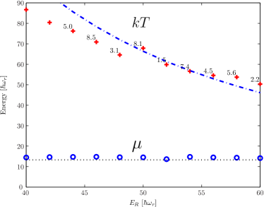
Figure 14: (Color online) Field temperatures and chemical potentials reached as a function of cutoff. Dashed and dash-dot lines indicate the predictions of Eq. (30) and Eq. (33) respectively. Measurement times are indicated as in Fig. 11.

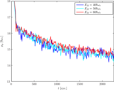
Figure 15: (Color online) Decay of the effective condensate chemical potential (as defined in Sec. V.3) for trajectories with initial chemical potential $\mu_{\mathrm{i}}=20\hbar\omega_{r}$ and three different values of the energy cutoff $E_{\mathrm{R}}$.

In Fig. 14 we plot the temperatures and chemical potentials attained in simulations with $\mu_{\mathrm{i}}=20$ and cutoff heights $E_{\mathrm{R}}$ varying over the range $2\mu_{\mathrm{i}}\rightarrow 3\mu_{\mathrm{i}}$. We note first that while the temperature shows a clear dependence on $E_{\mathrm{R}}$, the chemical potential appears relatively insensitive to it. The system therefore reaches a chemical potential closest to that resulting from the idealised transformation of the condensate to a lattice state without loss of atoms from the condensate mode. The measured temperature decreases with increasing cutoff as expected, but differs from the $T\propto 1/(\mathcal{M}-1)$ behaviour predicted by for a classical field in the Bogoliubov limit. We attribute this to the constraint imposed by the low cutoff. The cutoff here serves to increase the energy of natural modes in the system, by increasing their overlap with the condensate (c.f. the discussion in Sec. V.3), thus lowering the equilibrium temperature of those modes. Indeed for $E_{\mathrm{R}}=2\mu$, the classical turning point $r_{\mathrm{tp}}\sim 1.7r_{\mathrm{TF}}$, where $r_{\mathrm{TF}}\approx 7.8r_{0}$ is the TF radius of the lattice state, and so the corruption the quasiparticle mode shapes may be quite pronounced.

IX.0.2 Damping

As noted in Sec. V.4, it is difficult to extract quantitative comparisons of relaxation rates from the damping of vortex motion. Here we consider the relaxation of another quantity: the effective condensate chemical potential (power spectrum peak) $\mu_{\mathrm{p}}$ introduced in Sec. V.3. In Fig. 15, we show the decay of this quantity with time for three values of the cutoff $E_{\mathrm{R}}$. We observe that the damping is reasonably insensitive to the cutoff. A possible explanation for this behaviour is that as the effect of lowering the cutoff is to decrease the number of thermally occupied modes in the system and consequently to increase the temperature of these modes, that these two effects serve to approximately cancel one another in determining the rates of thermal damping.

References

- (1) K.W. Madison, F. Chevy, W. Wohlleben, and J. Dalibard, Phys. Rev. Lett. 84, 806 (2000).
- (2) K.W. Madison, F. Chevy, V. Bretin, and J. Dalibard, Phys. Rev. Lett. 86, 4443 (2001).
- (3) J. R. Abo-Shaeer, C. Raman, J. M. Vogels, and W. Ketterle, Science 292, 476 (2001).
- (4) J. R. Abo-Shaeer, C. Raman, and W. Ketterle, Phys. Rev. Lett. 88, 070409 (2002).
- (5) C. Raman, J. R. Abo-Shaeer, J. M. Vogels, K. Xu, and W. Ketterle, Phys. Rev. Lett. 87, 210402 (2001).
- (6) P. C. Haljan, I. Coddington, P. Engels, and E. A. Cornell, Phys. Rev. Lett. 87, 210403 (2001).
- (7) E. Hodby, G. Hechenblaikner, S. A. Hopkins, O. M. Marago, C. J. Foot, Phys. Rev. Lett. 88, 010405 (2001).
- (8) A. A. Penckwitt, R. J. Ballagh, and C. W. Gardiner, Phys. Rev. Lett. 89, 260402 (2002).
- (9) J. E. Williams, E. Zaremba, B. Jackson, T. Nikuni, A. Griffin, Phys. Rev. Lett. 88, 070401 (2002).
- (10) A. S. Bradley, C. W. Gardiner, and M. J. Davis, Phys. Rev. A 77, 033616 (2008).
- (11) K. Kasamatsu, M. Tsubota, and M. Ueda, Phys. Rev. A 67, 033610 (2003).
- (12) S. Sinha and Y. Castin, Phys. Rev. Lett. 87, 190402 (2001).
- (13) A. Recati, F. Zambelli, and S. Stringari, Phys. Rev. Lett. 86, 377 (2001).
- (14) N. G. Parker, R. M. W. van Bijnen, and A. M. Martin, Phys. Rev. A 73, 061603(R) (2006).
- (15) M. Tsubota, K. Kasamatsu, and M. Ueda, Phys. Rev. A 65, 023603 (2002).
- (16) S. Choi, S. A. Morgan, and K. Burnett, Phys. Rev. A 57, 4057 (1998).
- (17) B. Jackson and E. Zaremba, Phys. Rev. Lett. 87, 100404 (2001).
- (18) N. G. Parker and C. S. Adams, J. Phys. B 39, 43 (2006).
- (19) N. G. Parker and C. S. Adams, Phys. Rev. Lett. 95, 145301 (2005).
- (20) D. L. Feder, A. A. Svidzinsky, A. L. Fetter, and C. W. Clark, Phys. Rev. Lett. 86, 564 (2001).
- (21) E. Lundh, J.-P. Martikainen, and K.-A. Suominen, Phys. Rev. A 67, 063604 (2003).
- (22) M. J. Steel et al., Phys. Rev. A 58, 4824 (1998).
- (23) M. J. Davis, S. A. Morgan, and K. Burnett, Phys. Rev. Lett. 87, 160402 (2001).
- (24) A. Sinatra, C. Lobo, and Y. Castin, Phys. Rev. Lett. 87, 210404 (2001).
- (25) A. Sinatra, C. Lobo, and Y. Castin, J. Phys. B 35, 3599 (2002).
- (26) C. W. Gardiner, J. R. Anglin, and T. I. A. Fudge, J. Phys. B 35, 1555 (2002).
- (27) P. B. Blakie and M. J. Davis, Phys. Rev. A 72, 063608 (2005).
- (28) M. J. Davis and P. B. Blakie, Phys. Rev. Lett. 96, 060404 (2006).
- (29) T. P. Simula and P. B. Blakie, Phys. Rev. Lett. 96, 020404 (2006).
- (30) T. P. Simula, M. J. Davis, and P. B. Blakie, Phys. Rev. A 77, 023618 (2008).
- (31) R. N. Bisset, M. J. Davis, T. P. Simula, and P. B. Blakie, http://arXiv.org 0804.0286 (2008).
- (32) S. Wüster et al., Phys. Rev. A 75, 043611 (2007).
- (33) K. Gawryluk, M. Brewczyk, M. Gajda, and K. Rzażewski, Phys. Rev. A 76, 013616 (2007).
- (34) C. Lobo, A. Sinatra, and Y. Castin, Phys. Rev. Lett. 92, 020403 (2004).
- (35) S. Stock, Z. Hadzibabic, B. Battelier, M. Cheneau, J. Dalibard, Phys. Rev. Lett. 95, 190403 (2005).
- (36) D. S. Petrov, M. Holzmann, and G. V. Shlyapnikov, Phys. Rev. Lett. 84, 2551 (2000).
- (37) C. W. Gardiner and M. J. Davis, J. Phys. B 36, 4731 (2003).
- (38) A. S. Bradley, P. B. Blakie, and C. W. Gardiner, J. Phys. B 38, 4259 (2005).
- (39) A. S. Bradley and C. W. Gardiner, arXiv:cond-mat 0602162 (2006).
- (40) By far the most comprehensive prescription for the addition of noise to the initial states of TW-type simulations is that developed in Sinatra00 ; Sinatra01 ; Sinatra02 , which includes fluctuations in condensate occupation to second-order in the -symmetry preserving expansion of Ref. Castin98 . .
- (41) C. W. Gardiner, Phys. Rev. A 56, 1414 (1997).
- (42) Y. Castin and R. Dum, Phys. Rev. A 57, 3008 (1998).
- (43) M. O. Scully and M. S. Zubairy, Quantum Optics (Cambridge University Press, Cambridge, 1997).
- (44) A. Sinatra, Y. Castin, and C. Lobo, J. Mod. Opt. 47, 2629 (2000).
- (45) Y. Castin and R. Dum, Phys. Rev. Lett. 79, 3553 (1997).
- (46) J. Smit, Introduction to Quantum Fields on a Lattice (Cambridge University Press, Cambridge, 2002).
- (47) Above cutoff corrections are included in Gardiner03 where the dynamics are driven by a stationary above-cutoff thermal bath, and in Davis06 where only equilibrium properties of the system are considered. Neither of these conditions apply in the scenario considered here.
- (48) N. G. Parker, Ph.D. thesis, 2004.
- (49) W. H. Press, S. A. Teukolsky, W. T. Vetterling, and B. P. Flannery, Numerical Recipes in C, ed. (Cambridge University Press, Cambridge, 1992).
- (50) The central issue is the evaluation of the interaction term in the GPE evolution. A non-trivial modification of the method Davis_DPhil promotes it to a projective method based on exact numerical quadrature, with a formal energy cutoff.
- (51) C. W. Gardiner and P. Zoller, Handbook of Stochastic Methods, ed. (Springer-Verlag, Berlin, 2000).
- (52) R. J. Ballagh, Computational methods for nonlinear partial differential equations, http://www.physics.otago.ac.nz/research/jackdodd/resources/comp_lecture_ballagh.html, 2000.
- (53) M. J. Davis, DPhil. thesis, 2001.
- (54) In this and other simulations we have observed a tendency of vortices to cluster together in (short-lived) co-rotating pairs which orbit their geometric centre, a behaviour characteristic of two-dimensional superfluid turbulence (see Wang07 and references therein).
- (55) E. B. Sonin, Rev. Mod. Phys. 59, 87 (1987).
- (56) R. J. Donnelly, Quantized Vortices in Helium II (Cambridge University Press, Cambridge, 1991).
- (57) P. O. Fedichev, G. V. Shlyapnikov, and J. T. M. Walraven, Phys. Rev. Lett. 80, 2269 (1998).
- (58) S. Giorgini, Phys. Rev. A 57, 2949 (1998).
- (59) L. P. Pitaevskii and S. Stringari, Phys. Lett. A 235, 398 (1997).
- (60) R. Z. Sagdeev, D. A. Usikov, and G. M. Zaslavsky, Nonlinear Physics: From the Pendulum to Turbulence and Chaos, Contemporary Concepts in Physics (Harwood Academic, Chur, 1988).
- (61) A. Sinatra, P. O. Fedichev, Y. Castin, J. Dalibard, G. V. Shlyapnikov, Phys. Rev. Lett. 82, 251 (1999).
- (62) F. Dalfovo, S. Giorgini, L. P. Pitaevskii, and S. Stringari, Rev. Mod. Phys. 71, 463 (1999).
- (63) A. J. Leggett, Rev. Mod. Phys. 73, 307 (2001).
- (64) P. O. Fedichev and G. V. Shlyapnikov, Phys. Rev. A 60, R1779 (1999).
- (65) This energy change cannot be attributed to the initial trap deformation associated with the stirrer, as the energy of an axially symmetry state is unchanged by the abrupt introduction of a perturbation of quadrupolar symmetry (i.e., within the sudden approximation Bransden00 implicit in our procedure).
- (66) S. Giorgini, L. P. Pitaevskii, and S. Stringari, J. Low Temp. Phys. 109, 309 (1997).
- (67) M. Naraschewski and D. M. Stamper-Kurn, Phys. Rev. A 58, 2423 (1998).
- (68) R. K. Pathria, Statistical Mechanics, ed. (Butterworth-Heinemann, Oxford, 1996).
- (69) Y. Castin, in Coherent Atomic Matter Waves, Vol. 72 of Les Houches - Ecole d’Ete de Physique Theorique, edited by R. Kaiser, C. Westbrook, and F. David (EDP Sciences and Springer-Verlag, Berlin, Heidelberg, New York, 2001), p. 1.
- (70) V. Bagnato, D. E. Pritchard, and D. Kleppner, Phys. Rev. A 35, 4354 (1987).
- (71) For small basis sizes and low temperatures, however, the discrete nature of the true spectrum becomes important and the underlying semiclassical approximation becomes invalid, and so the fits obtained become poor for the smallest condensates we consider.
- (72) We note than in Holzmann07 , the fully bosonic analogue of Eq. (V.1.2) was derived as a self-consistent mean-field description of the total field density in the local density approximation as the BKT transition is approached from above.
- (73) Condensates formed in dilute Bose gases may possess some angular momentum without containing vortices due to their surface oscillations (see e.g. Stringari96 ).
- (74) F. Zambelli and S. Stringari, Phys. Rev. A 63, 033602 (2001).
- (75) J. J. García-Ripoll and V. M. Pérez-García, Phys. Rev. A 64, 013602 (2001).
- (76) D. L. Feder and C. W. Clark, Phys. Rev. Lett. 87, 190401 (2001).
- (77) D. E. Sheehy and L. Radzihovsky, Phys. Rev. A 70, 051602(R) (2004).
- (78) A. A. Norrie, R. J. Ballagh, and C. W. Gardiner, Phys. Rev. Lett. 94, 040401 (2005).
- (79) A. A. Norrie, R. J. Ballagh, and C. W. Gardiner, Physical Review A (Atomic, Molecular, and Optical Physics) 73, 043617 (2006).
- (80) A. A. Norrie, R. J. Ballagh, C. W. Gardiner, and A. S. Bradley, Physical Review A (Atomic, Molecular, and Optical Physics) 73, 043618 (2006).
- (81) C. W. Gardiner and P. Zoller, Quantum Noise, ed. (Springer-Verlag, Berlin, 2000).
- (82) M. Lewenstein and L. You, Phys. Rev. Lett. 77, 3489 (1996).
- (83) O. Penrose and L. Onsager, Phys. Rev. 104, 576 (1956).
- (84) R. Seiringer, arXiv:cond-mat 0801.0427 (2008).
- (85) M. J. Davis, S. A. Morgan, and K. Burnett, Phys. Rev. A 66, 053618 (2002).
- (86) M. Brewczyk, P. Borowski, M. Gajda, and K. Rza̧żewski, J. Phys. B 37, 2725 (2004).
- (87) It is important to note that such an artifact must arise in any field theory which is truncated either explicitly or implicitly, and that the defect occurring here is thus close to the minimal defect attainable in such a description.
- (88) A. Bezett, E. Toth, and P. B. Blakie, Phys. Rev. A 77, 023602 (2008).
- (89) C. F. Barenghi, R. J. Donnelly, and W. F. Vinen, Quantized Vortex Dynamics and Superfluid Turbulence (Springer-Verlag, Berlin, 2001).
- (90) While additional numerical procedures were used in calculations presented in Parker06b ; Parker05a , these additions were not essential for lattice crystallization, i.e., relaxation to a lattice state was also observered in simulations performed without these additions note15 .
- (91) The finite difference operator defined Parker_PhD constitutes a good approximation to the (1D) Laplacian for variations in on scales large compared to , i.e., for wavenumbers small compared to the natural grid (Nyquist) cutoff . Conversely, for wavenumbers which are larger (yet still smaller than ), such as may arise in turbulent or thermal fields, the action of this approximate Laplacian is corrupted. By contrast, in (aliasing) Fourier-based methods Lundh03 , the Laplacian defined posesses a complete basis of exact eigenfunctions within the simulation window, and its action is thus consistent across its (periodic) domain. DVR methods Feder01a ; Schneider99 similarly provide for the accurate evaluation of the Laplacian, and projective methods serve to retain analogous properties within more carefully delimited simulation windows.
- (92) We note that our calculations confirm that in the absence of trap anisotropy and therefore without any dynamical instability, the presence of Wigner noise will eventually allow a condensate propagated in the rotating frame to nucleate vortices.
- (93) An alternate (and contrary) explanation, that the field is exhibiting quasi-recurrent behaviour in the manner of Fermi65 seems unlikely given that the trajectories appear to have converged to the temperatures predicted by the simple analysis presented in Sec. V.1.
- (94) E. Lundh, C. J. Pethick, and H. Smith, Phys. Rev. A 58, 4816 (1998).
- (95) Y. Kagan, E. L. Surkov, and G. V. Shlyapnikov, Phys. Rev. A 54, R1753 (1996).
- (96) Y. Castin and R. Dum, Phys. Rev. Lett. 77, 5315 (1996).
- (97) J. W. Robinson, Atomic Spectroscopy, ed. (Marcel Dekker, New York, 1996).
- (98) A. Posazhennikova, Rev. Mod. Phys. 78, 1111 (2006).
- (99) At a late stage in the preparation of this manuscript we became aware of experimental investigations into the nature of Bose-condensates in rotating, quasi-2D geometries Lamporesi08 .
- (100) A. M. Cohen, Numerical Analysis (Halsted, United Kingdom, 1973), Vol. 1.
- (101) S. Wang, Y. A. Sergeev, C. F. Barenghi, and M. A. Harrison, J. Low Temp. Phys. 149, 65 (2007).
- (102) B. H. Bransden and C. J. Joachain, Quantum Mechanics, ed. (Pearson Education, Essex, 2000).
- (103) M. Holzmann, G. Baym, J.-P. Blaizot, and F. Laloe, Proceedings of the National Academy of Sciences 104, 1476 (2007).
- (104) S. Stringari, Phys. Rev. Lett. 76, 1405 (1996).
- (105) N. G. Parker and C. S. Adams (private communication).
- (106) B. I. Schneider and D. L. Feder, Phys. Rev. A 59, 2232 (1999).
- (107) E. Fermi, J. Pasta, and S. Ulam, in Collected Papers of Enrico Fermi, edited by E. Segré (University of Chicago Press, Chicago, 1965).
- (108) G. Lamporesi, poster at ICAP2008, Storrs, CT, USA.