Effects of Strong Correlations on the Zero Bias Anomaly in the Extended Hubbard Model with Disorder

Abstract

We study the effect of strong correlations on the zero bias anomaly (ZBA) in disordered interacting systems. We focus on the two-dimensional extended Anderson-Hubbard model, which has both on-site and nearest-neighbor interactions on a square lattice. We use a variation of dynamical mean field theory in which the diagonal self-energy is solved self-consistently at each site on the lattice for each realization of the randomly-distributed disorder potential. Since the ZBA occurs in systems with both strong disorder and strong interactions, we use a simplified atomic-limit approximation for the diagonal inelastic self-energy that becomes exact in the large-disorder limit. The off-diagonal self-energy is treated within the Hartree-Fock approximation. The validity of these approximations is discussed in detail. We find that strong correlations have a significant effect on the ZBA at half filling, and enhance the Coulomb gap when the interaction is finite-ranged.

I Introduction

The term “zero bias anomaly” (ZBA) refers either to a peak in, or a suppression of, the density of states (DOS) at the Fermi energy. In disordered materials, a ZBA arises from the interplay between disorder and interactions. Zero bias anomalies were originally predicted to occur in strongly-disordered insulators by Efros and ShklovskiiEfros and Shklovskii (1975); Efros (1976) (ES) and later in weakly-disordered metals by Altshuler and AronovAltshuler and Aronov (1985) (AA). In the limit of weak interactions and disorder, AA showed that the exchange self-energy of the screened Coulomb interaction produces a cusp-like minimum in the DOS at the Fermi energy. In the limit of strong disorder, ES showed that the classical Hartree self-energy of the unscreened Coulomb interaction causes the DOS to vanish at the Fermi energy. Experiments have shown a smooth evolution between the AA and ES limits as a function of disorder,Butko, DiTusa, and Adams (2000) and it appears that the essential physics of the ZBA in conventional metals and insulators is well understood.

In this work, we are interested in anomalies which have been observed in a number of transition metal oxide materials, where the physics is less well understood. Transition metal oxides often exhibit unconventional behavior because the physics of their valence band is dominated by strong short-ranged interactions whose effects cannot generally be explained by conventional theories of metals and insulators. Most notably, many transition metal oxides exhibit a Mott transition when their valence band is half-filled. In disorder-free systems, the Mott transitionDagotto (1994); Imada et al. (1998) occurs between a gapless metallic state and a gapped insulating state, and is driven by a strong intraorbital Coulomb interaction.

The Mott transition may occur as a function of any number of parameters,Imada et al. (1998) such as temperatureMorin1959 or magnetic field,Hanasaki et al. (2006) but more commonly occurs in transition-metal oxides as a result of chemical doping. A number of experimentsSarma et al. (1998); Ino et al. (2004); Kim et al. (2006); Nakatsuji et al. (2004); Kim et al. (2005) have found that chemical doping introduces sufficient disorder that there is a regime between the Mott-insulating and gapless phases that is characterized by a ZBA. This naturally raises the question of how the strong electron-electron correlations that are prevalent in the gapless phase near the Mott transition affect the physics of the ZBA.

The effect of strong correlations on the ZBA has received little attention.discussed In large part, this is due to the difficulty of incorporating both strong correlations and disorder in a manageable theory. A number of calculations based on the unrestricted Hartree-Fock approximation (HFA) have been used to study the phase diagram of the disordered Hubbard model.Milovanovic1989 ; Tusch1993 ; Heidarian2004a ; Fazileh, Gooding, Atkinson, and Johnson (2006) In these calculations, the disorder potential is treated exactly for finite-sized systems, but the intraorbital Coulomb interaction is treated at the mean-field level and therefore neglects strong correlations. Much of the recent progress has involved various formulations of dynamical mean field theory (DMFT) to include disorder at some level of approximation. Coherent-potential-like approximations have been employed by a variety of authors.Ulmke et al. (1995); Laad et al. (2001); Dobrosavljević et al. (2003); Byczuk et al. (2005); Balzer and Potthoff (2005); Lombardo et al. (2006) In these calculations, the local electron self-energy contains both inelastic contributions from the interactions and elastic contributions from the disorder-averaging process. It is well known that these kinds of disorder-averaging approximations capture many features of the DOS but do not retain the nonlocal correlations responsible for the ZBA and cannot, therefore, explain the experiments cited above.Altshuler and Aronov (1985) An extension of DMFT, called statistical DMFT, has been employed to study ensembles consisting of Bethe lattices with random site energies. Dobrosavljević and Kotliar (1997); Miranda and Dobrosavljević (2005) This represents an improvement over the disorder-averaged approximations in that the results depend nontrivially on the coordination number of the Bethe lattice. Very recently, the DMFT equations have been solved by us on a two dimensional square lattice in a way which preserves spatial correlations between sites.Song et al. (2007) The calculations employed a simple atomic-limit approximation for the self-energy that, while generally appropriate for the large-disorder limit, does not contain the off-diagonal self-energies responsible for the DOS anomalies observed in experiments.

In this work, we extend our earlier calculations to include a nearest neighbour interaction $V$. This interaction is treated at the mean-field level, and serves two purposes in this work: First, it represents finite range interactions which are present in real materials. Second, the exchange self-energy coming from this interaction plays a qualitatively similar role to the off-diagonal self-energy that is missing in our treatment of the intraorbital interaction $U$. The intraorbital self-energy is calculated within a Hubbard-I (HI) approximation which has the effect of suppressing double occupancy of orbitals. Details of these calculations are outlined in Sec. II.1. Because the HI approximation is known to be defficient in the disorder-free limit, we include a discussion in Sec. II.2 showing that the approximation for the diagonal self-energy is valid in the limit of large disorder and low coordination number. In Sec. II.3, we introduce a coherent potential approximation (CPA) for the disordered Hubbard model which is used as a point of comparison for the lattice DMFT calculations. The results of numerical and analytical calculations are presented in Sec. III.

Our primary result is that the ZBA is strongly enhanced by electron correlations near half-filling when the interaction is finite-ranged. The ZBA is predominantly of the ES type, in the sense that the largest contribution is from the classical Hartree interaction between localized charges on neighboring sites. The enhancement of the ZBA at half-filling is due to strong correlations which inhibit screening of the impurity potential: Near the Mott transition, the absence of screening drives the system towards the strongly localized limit where the physics of the Coulomb gap is most important. The magnitude of the ZBA is doping dependent, and drops off away from half-filling.

II Calculations

II.1 Method

We study an extended Anderson-Hubbard model, also known as a disordered $t$-$U$-$V$ model. In this model, $t$ denotes the electron kinetic energy, $U$ the intraorbital Coulomb interaction, and $V$ the interaction between nearest-neighbor sites. The $V$-term in the Hamiltonian can be used to represent two distinct physical processes. First, it represents the nonlocal Coulomb interaction that, while neglected in the Hubbard model, is generally present in real materials. Second, as shown below, the exchange self-energy from the nonlocal interaction is qualitatively similar to the exchange self-energy that arises in a perturbative treatment of the Hubbard model. This effective interaction plays a crucial role in clean low-dimensional systems.Lieb1968 ; Hirsch1985 ; White1989 ; Otsuka2000 It is often treated explicitly in the large-$U$ limit via an approximate mapping of the Hubbard model onto the $t$-$J$ model, where $J$ is the strength of the effective nonlocal interaction. A major difference between the $t$-$J$ and extended Anderson-Hubbard models is that double occupation of orbitals is completely suppressed in the former whereas a finite fraction of sites will be doubly occupied in the latter when the width of the disorder distribution is larger than $U$.

The extended Anderson-Hubbard model is

$$\hat{H} = -t\sum_{\langle i,j\rangle,\sigma}c^{\dagger}_{i\sigma}c_{j\sigma}+\frac{V}{2}\sum_{\langle i,j\rangle}\hat{n}_{i}\hat{n}_{j}$$ (1)

$$+\sum_{i}\left(\epsilon_{i}\hat{n}_{i}+U\hat{n}_{i\uparrow}\hat{n}_{i\downarrow}\right),$$

where $\langle i,j\rangle$ denotes nearest-neighbor lattice sites $i$ and $j$, $\hat{n}_{i\sigma}=c^{\dagger}_{i\sigma}c_{i\sigma}$, $\hat{n}_{i}=\hat{n}_{i\uparrow}+\hat{n}_{i\downarrow}$, and parameters $t$, $U$ and $V$ are the kinetic energy, the on-site Coulomb interaction, and the nearest-neighbor interaction respectively. $\epsilon_{i}$ is the site energy, which is box-distributed according to $P(\epsilon_{i})=W^{-1}\Theta(W/2-|\epsilon_{i}|)$, where $W$ is the width of the disorder distribution and $\Theta(x)$ the step-function.

We treat the nearest-neighbor interaction at the mean-field level:

$$\frac{V}{2}\hat{n}_{i}\hat{n}_{j}\approx V\left(\hat{n}_{i}n_{j}-\sum_{\sigma}c^{\dagger}_{i\sigma}c_{j\sigma}f_{ji}+f_{ij}^{2}-\frac{n_{i}n_{j}}{2}\right)$$ (2)

with $f_{ji}=\langle c^{\dagger}_{j\uparrow}c_{i\uparrow}\rangle=\langle c^{\dagger}_{j\downarrow}c_{i\downarrow}\rangle$ in the paramagnetic phase and $n_{j}=\langle\hat{n}_{j}\rangle$. Both $f_{ij}$ and $n_{j}$ are determined self-consistently. The mean-field Hamiltonian, up to an additive constant, is:

$$\hat{H}=\sum_{\langle i,j\rangle\sigma}t_{ij}^{\prime}c^{\dagger}_{i\sigma}c_{j\sigma}+\sum_{i}\epsilon_{i}^{\prime}\hat{n}_{i}+U\sum_{i}\hat{n}_{i\uparrow}\hat{n}_{j\downarrow}$$ (3)

where $t_{ij}^{\prime}=-t-Vf_{ij}$ and $\epsilon_{i}^{\prime}=\epsilon_{i}+V\sum_{j}n_{j}$, where the sum is over nearest neighbors of $i$.

The approximate Hamiltonian (3) is then solved using an iterative lattice DMFT (LDMFT) method that captures the strong-correlation physics of the intraorbital interaction.others On an $N$-site lattice, the single-particle Green’s function can be expressed as an $N\times N$ matrix in the site-index:

$${\bf G}(\omega)=[\omega{\bf I}-{\bf t}-{\boldsymbol{\epsilon}}-{\bf\Sigma}(\omega)]^{-1}$$ (4)

with ${\bf I}$ the identity matrix, ${\bf t}$ the matrix of renormalized hopping amplitudes $t_{ij}^{\prime}$, ${\boldsymbol{\epsilon}}$ the diagonal matrix of renormalized site energies $\epsilon_{i}^{\prime}$ and ${\bf\Sigma}(\omega)$ the matrix of local self-energies. The self-energy $\Sigma_{i}(\omega)$ corresponds to the inelastic self-energy $\Sigma(\omega)$ (the so-called “impurity self-energy”) in standard DMFT, which is obtained by various self-consistent impurity solvers.Kotliar1996 The iteration cycle begins with the calculation of ${\bf G}(\omega)$ from Eq. (4), and $n_{i\sigma}$ and $f_{ij}$ given by,

$$n_{i\sigma} = -\frac{1}{\pi}\int_{-\infty}^{\varepsilon_{F}}d\omega\mathrm{Im}G_{ii}(\omega)$$ (5)

$$f_{ij} = -\frac{1}{\pi}\int_{-\infty}^{\varepsilon_{F}}d\omega\mathrm{Im}G_{ji}(\omega).$$ (6)

from the previous iteration. For each site $i$, one defines a Weiss mean field ${\cal G}^{0}_{i}(\omega)=[G_{ii}(\omega)^{-1}+\Sigma_{i}(\omega)]^{-1}$ where $G_{ij}(\omega)$ are the matrix elements of ${\bf G}(\omega)$. The HI approximation is the simplest improvement over the HFA that generates both upper and lower Hubbard bands and, as we discuss in the next section, it works well in the large-disorder limit $W\gg t$. In this approximation, ${\cal G}_{i}(\omega)=\left[{\cal G}^{0}_{i}(\omega)^{-1}-\Sigma_{i}^{HI}(\omega)\right]^{-1}$ where

$$\Sigma_{i}^{HI}(\omega)=U\frac{n_{i}}{2}+\frac{U^{2}\frac{n_{i}}{2}(1-\frac{n_{i}}{2})}{\omega-\epsilon_{i}^{\prime}-U(1-\frac{n_{i}}{2})},$$ (7)

and $n_{i}$ is self-consistently determined for each site.caveat

We remark that we can also express the Green’s function as

$${\bf G}(\omega)=[\omega{\bf I}-{\bf t_{0}}-{\boldsymbol{\epsilon}_{0}}-{\bf\Sigma}(\omega)]^{-1}$$ (8)

where $\bf t_{0}$ and $\boldsymbol{\epsilon}_{0}$ are matrices of the unrenormalized hopping amplitudeds and site energies. In this case, the self-energy is:

$$\Sigma_{ii}=U\frac{n_{i}}{2}+V\sum_{j}n_{j}+\frac{\displaystyle U^{2}\frac{n_{i}}{2}(1-\frac{n_{i}}{2})}{\displaystyle\omega-\epsilon_{i}-U(1-\frac{n_{i}}{2})-V\sum_{j}n_{j}}$$ (9a)

and

$$\Sigma_{ij}=-Vf_{ij}.$$ (9b)

This form emphasizes the nonlocal nature of the self-energy.

II.2 Validity of the Self-Energy

In this section, we discuss our treatment of the intraorbital interaction in the renormalized Hamiltonian (3). We show that Eq. (7) is a reasonable approximation for the local self-energy in the large-disorder limit provided that nonlocal effective interactions generated by $U$ can be absorbed into the interaction $V$.

Our discussion is based on a two-site Anderson-Hubbard Hamiltonian, ie. on Eq. (3) with two sites labelled “1” and “2”. This Hamiltonian can, of course, be diagonalized exactly with relatively little effort. Here, we are interested in developing an approximate treatment that is valid in the large disorder limit, and which can be applied to the $N$-site problem. Comparison to the exact solution is used as a benchmark for the approximation.

We use an equation-of-motion method to arrive at approximate expressions for the single-particle Green’s function. Defining a Liouvillian superoperator ${\cal L}$ such thatFulde

$${\cal L}\hat{A}\equiv[\hat{H},\hat{A}],$$ (10)

where $\hat{A}$ is an arbitrary operator, we can formally write the time evolution of $\hat{A}$ as $\hat{A}(t)=\exp(i{\cal L}t)\hat{A}(0)$. It follows directly that the retarded Green’s function can be written

$$G_{i\sigma,j\sigma}(\omega)=(c^{\dagger}_{i\sigma}|\frac{1}{\omega-{\cal L}}c^{\dagger}_{j\sigma})$$ (11)

where the inner product of two operators is defined as $(\hat{A}|\hat{B})=\langle\{\hat{A}^{\dagger},\hat{B}\}\rangle$ and $\{,\}$ refers to the anticommutator. The operator set $c_{i\sigma}^{\dagger}$ is not closed under operations by ${\cal L}$, but a complete operator set can be generated with repeated operation by ${\cal L}$ on $c_{i\sigma}^{\dagger}$. For example,

$${\cal L}c_{i\sigma}^{\dagger}=\epsilon_{i}^{\prime}c_{i\sigma}^{\dagger}+\sum_{j}c_{j\sigma}^{\dagger}t_{ji}^{\prime}+U(b^{\dagger}_{i\sigma}-c_{i\sigma}^{\dagger}n_{i\overline{\sigma}})$$ (12)

where $b^{\dagger}_{i\sigma}=c_{i\sigma}^{\dagger}(\hat{n}_{i\overline{\sigma}}-n_{i\overline{\sigma}})$ and $\overline{\sigma}=-\sigma$. The operator $b^{\dagger}_{i\sigma}$ is a composite operator, and further composite operators can be generated from ${\cal L}^{2}c_{i\sigma}^{\dagger}$, etc. The higher order composite operators involve excitations on multiple lattice sites, and are therefore expected to be less important in the disordered case than in the clean limit. Here, we truncate the series after a single application of ${\cal L}$ so that our operator basis consists of two operators, $c_{i\sigma}^{\dagger}$ and $b_{i\sigma}^{\dagger}$, for each site and spin. This leads to a “two-pole” approximation for the Green’s function. This approach has been studied at length in the clean limit and has been shown to provide a reasonable qualitative description of the Hubbard model.Mehlig1995 ; Grober2000 ; Avella2004 As shown in Fig. 1, the two-pole approximation (described in more detail below) is essentially indistinguishable from the exact solution for the DOS of the two-site system.

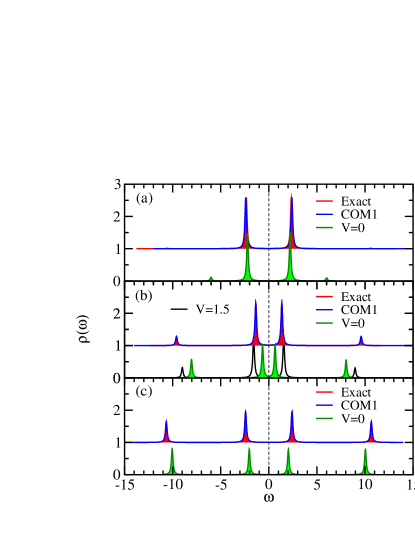
Figure 1: (Color online) Comparison of the approximate and exact densities of states for a two-site system. The site energies are $\epsilon_{1}=W/2$, $\epsilon_{2}=-W/2$ for $W=8t$. Figure panels are for (a) $U=4t$, (b) $U=8t$ and (c) $U=12t$. Exact calculations are based on exact diagonalization of the two-site Hubbard model. Approximate densities of states are given by $\rho(\omega)=-\mbox{Im}\sum_{i}G_{ii}(\omega)/\pi$, with ${\bf G}(\omega)$ the matrix (19). Two different approximations are made for the self energies: the first has the self energy given by Eq. (20) and makes the COM1 approximation for $p$;Avella2004 the second has the self energy given by Eq. (9b) with different choices for $V$. Both the COM1 and exact solutions are offset for clarity. The COM1 solution is essentially indistinguishable from the exact solution in all cases. Note that $\varepsilon_{F}$ is the zero of energy in this and all other figures.

It is useful to define a generalized Green’s function in the expanded operator space:

$${\cal G}_{i\sigma,j\sigma}(\omega)=\left[\begin{array}[]{cc}(c^{\dagger}_{i\sigma}|\frac{1}{\omega-{\cal L}}c^{\dagger}_{j\sigma})&(c^{\dagger}_{i\sigma}|\frac{1}{\omega-{\cal L}}b^{\dagger}_{j\sigma})\\[8.53581pt] (b^{\dagger}_{i\sigma}|\frac{1}{\omega-{\cal L}}c^{\dagger}_{j\sigma})&(b^{\dagger}_{i\sigma}|\frac{1}{\omega-{\cal L}}b^{\dagger}_{j\sigma})\end{array}\right]$$ (13)

such that $G_{i\sigma,j\sigma}(\omega)$ is given by the upper left quadrant of ${\cal G}_{i\sigma,j\sigma}(\omega)$. Defining the Liouvillian matrix,

$$L_{i\sigma,j\sigma}(\omega)=\left[\begin{array}[]{cc}(c^{\dagger}_{i\sigma}|{\cal L}c^{\dagger}_{j\sigma})&(c^{\dagger}_{i\sigma}|{\cal L}b^{\dagger}_{j\sigma})\\[5.69054pt] (b^{\dagger}_{i\sigma}|{\cal L}c^{\dagger}_{j\sigma})&(b^{\dagger}_{i\sigma}|{\cal L}b^{\dagger}_{j\sigma})\end{array}\right],$$ (14)

and the matrix of overlap integrals,

$$\chi_{i\sigma,j\sigma}=\left[\begin{array}[]{cc}(c^{\dagger}_{i\sigma}|c^{\dagger}_{j\sigma})&(c^{\dagger}_{i\sigma}|b^{\dagger}_{j\sigma})\\[5.69054pt] (b^{\dagger}_{i\sigma}|c^{\dagger}_{j\sigma})&(b^{\dagger}_{i\sigma}|b^{\dagger}_{j\sigma})\end{array}\right],$$ (15)

we get

$${\cal G}_{i\sigma,j\sigma}(\omega)=\sqrt{\chi_{i\sigma,i\sigma}}[\omega-\tilde{L}]^{-1}_{i\sigma,j\sigma}\sqrt{\chi_{j\sigma,j\sigma}}$$ (16)

with

$$\chi_{i\sigma,j\sigma}=\delta_{i,j}\left[\begin{array}[]{cc}1&0\\ 0&n_{i\overline{\sigma}}(1-n_{i\overline{\sigma}})\end{array}\right]$$ (17)

and $\tilde{L}=\sqrt{\chi^{-1}}L\sqrt{\chi^{-1}}$.

For the nonmagnetic case, up and down spins are equivalent, and only the former need be considered. For the two-site system, and taking the basis $[c_{1\uparrow}^{\dagger},c_{2\uparrow}^{\dagger},b_{1\uparrow}^{\dagger},b_{2\uparrow}^{\dagger}]$, we write the Liouvillian matrix explicitly as

$$\tilde{L}=\left[\begin{array}[]{cccc}\epsilon_{1}^{\prime}+Un_{1\downarrow}&-t^{\prime}&\tilde{U}_{1}&0\\ -t^{\prime}&\epsilon_{2}^{\prime}+Un_{2\downarrow}&0&\tilde{U}_{2}\\ \tilde{U}_{1}&0&\tilde{\epsilon}_{1}&-t^{\prime}\tilde{p}\\ 0&\tilde{U}_{2}&-t^{\prime}\tilde{p}&\tilde{\epsilon}_{2}\end{array}\right],$$ (18)

where

$$\tilde{U}_{i} = U\sqrt{n_{i\downarrow}(1-n_{i\downarrow})}$$

$$\tilde{\epsilon}_{i} = \epsilon_{i}^{\prime}+U(1-n_{i\downarrow})-t^{\prime}\tilde{\Delta}_{i}$$

$$\tilde{\Delta}_{i} = \Delta_{i}[n_{i\downarrow}(1-n_{i\downarrow})]^{-1}$$

$$\Delta_{i} = \langle(\hat{n}_{i\uparrow}-n_{i\downarrow})c^{\dagger}_{j\downarrow}c_{i\downarrow}\rangle-\langle(1-\hat{n}_{i\uparrow}-n_{i\downarrow})c^{\dagger}_{i\downarrow}c_{j\downarrow}\rangle$$

$$\tilde{p} = p[n_{1\downarrow}(1-n_{1\downarrow})n_{2\downarrow}(1-n_{2\downarrow})]^{-1/2}$$

$$p = \langle\hat{n}_{1\downarrow}\hat{n}_{2\downarrow}\rangle-n_{1\downarrow}n_{2\downarrow}-\langle c^{\dagger}_{1\uparrow}c_{2\uparrow}(c^{\dagger}_{2\downarrow}c_{1\downarrow}+c^{\dagger}_{1\downarrow}c_{2\downarrow})\rangle$$

In the expression for $\Delta_{i}$, $j$ is the nearest neighbor to $i$ (i.e. $j=1$ if $i=2$ and $j=2$ if $i=1$).

Equation [18] allows us to solve for the Green’s function, provided the fields $\Delta_{i}$, $p$, and $n_{i\downarrow}$ are known. In practice, $\Delta_{i}$ and $n_{i\downarrow}$ can be solved self-consistently, but further information is needed to calculate $p$.

The Green’s function $G(\omega)$ is given by the upper left $2\times 2$ quadrant of ${\cal G}(\omega)$. It is straightforward to solve Eq. (16) to show that

$$G(\omega)=\left[\begin{array}[]{cc}\omega-\epsilon_{1}^{\prime}-\Sigma_{11}(\omega)&t^{\prime}-\Sigma_{12}(\omega)\\ t^{\prime}-\Sigma_{21}(\omega)&\omega-\epsilon_{2}^{\prime}-\Sigma_{22}(\omega)\end{array}\right]^{-1}$$ (19)

with

$$\Sigma_{ii} = Un_{i\downarrow}+\frac{\tilde{U}_{i}^{2}(\omega-\tilde{\epsilon}_{j})}{(\omega-\tilde{\epsilon}_{1})(\omega-\tilde{\epsilon}_{2})-t^{\prime 2}\tilde{p}^{2}}$$ (20a)

$$\Sigma_{12} = \Sigma_{12}$$ (20b)

$$= \frac{-t^{\prime}U^{2}p}{(\omega-\tilde{\epsilon}_{1})(\omega-\tilde{\epsilon}_{2})-t^{\prime 2}\tilde{p}^{2}}$$

where $j$ is again the nearest neighbor to $i$. Equations [20a] and [20b] are the basic expressions for the self-energy. These expressions are shown in Fig. 1 to give very accurate results for the Green’s function provided that $p$ is correctly chosen. In this work, we have used the COM1 approximation of Avella and Mancini.Avella2004 The COM1 approximation works well for the simple inhomogeneous systems we have tested it on, but is extremely difficult to apply to disordered systems where $p$ is different along every bond in the lattice.

Some simplifications can be made in the case of large disorder. To begin with, we discuss the diagonal self-energies $\Sigma_{ii}$, and take $i=1$. We note that $\tilde{p}\sim O(1)$, so that

$$\Sigma_{11}\rightarrow Un_{1\downarrow}+\frac{U^{2}n_{1\downarrow}(1-n_{1\downarrow})}{\omega-\epsilon_{1}^{\prime}-U(1-n_{1\downarrow})+t^{\prime}\tilde{\Delta}_{1}},$$ (21)

whenever $(\omega-\tilde{\epsilon}_{1})(\omega-\tilde{\epsilon}_{2})\gg t^{2}$. Apart from the shift $t\tilde{\Delta}_{1}$, this is just the Hubbard-I approximation for the self-energy. As we show next, Eq. [21] is justified for $\omega\approx\varepsilon_{F}$ in the large disorder limit, which corresponds in the two-site problem to $|\epsilon_{1}-\epsilon_{2}|\gg t$.

We are interested in the validity of Eq. (21) near $\varepsilon_{F}$ and take the particular case $\varepsilon_{F}=U/2$ (which corresponds to half-filling) where strong correlations are most important. When $t=0$, each atomic Green’s function has poles at $\epsilon_{i}^{\prime}$ and $\epsilon_{i}^{\prime}+U$, so that spectral weight at $\varepsilon_{F}$ comes from sites with $\epsilon_{i}^{\prime}=\pm U/2$. This remains approximately true when $t\neq 0$ provided that $W\gg t$. Then, if site 1 contributes spectral weight at the Fermi level,

$$\varepsilon_{F}-\tilde{\epsilon}_{1}\sim U,$$

and Eq. (21) follows from Eq. (20a) provided $|\varepsilon_{F}-\tilde{\epsilon}_{2}|>t^{2}/U$. This condition will only not be met when $\epsilon_{2}^{\prime}\approx-U/2$. In other words, the two cases not well described by Eq. (21) are (i) $\epsilon_{1}^{\prime}\approx\epsilon_{2}^{\prime}$ and (ii) $\epsilon_{1}^{\prime}\approx\epsilon_{2}^{\prime}+U$.

Certainly, in any random distributed set of site energies, both cases are expected to occur for some fraction of sites on the lattice. However, if the disorder potential is large, and the coordination number of the lattice is low, then the probability of any given site having a nearest neighbor satisfying either condition (i) or (ii) is low, and the fraction of sites not described by Eq. (21) is small. It is interesting to note that the physical processes neglected here are (i) formation of singlet correlations between nearly degenerate sites and (ii) resonant exchange between sites in which the double occupancy of site 1 is nearly degenerate with singlet formation between sites 1 and 2.

Two further comments are warranted regarding our treatment of $\Sigma_{11}$. First, the simplifications made above assume that both $U$ and $W$ are large. This case is directly relevant to the current work since it is the regime in which density of states anomalies are observed. However, we have found empirically through numerical studies of small clusters that Eq. (21) is also a good approximation when $U$ is small. This point is illustrated in Fig. 1(a). Second, the term $t^{\prime}\Delta_{1}$ in Eq. (21) is neglected in Eq. (9a). In the clean limit, $|\Delta|\lesssim 0.2$ and depends only weakly on $U$.Avella2004 This term is small relative to the Hartree shift $V\sum_{j}n_{j}$ and is therefore neglected.

We emphasize that the Hartree shift $V\sum_{j}n_{j}$ does not arise naturally in our treatment of the Hubbard-$U$ interaction. It must therefore be undertstood to come directly from the nonlocal Coulomb interaction. This point is important because, as is shown in Sec. III, the Hartree term makes a large contribution to the ZBA at half-filling.

The off-diagonal self-energy is significantly harder to evaluate than the diagonal term. It requires knowledge of a quantity $p$ that cannot be calculated self-consistently within the two-pole approximation, although various approximate schemes exist for its evaluation.Avella2004 However, we note from the definition of $p$ that it measures exchange correlations between sites 1 and 2 and plays a similar role to the exchange self-energy $-Vf_{12}$ defined in Sec. II.1. This suggests that, qualitatively, the exchange self-energy may represent the exchange term from the nonlocal Coulomb interaction.

Figure 1 shows the DOS of a two-site system calculated within the approximation (9b). The main effect of $V$ is to produce a level repulsion between states above and below the Fermi energy, as illustrated in Fig. 1(b). The magnitude of the level repulsion decreases with increasing $U$, and is unobservably small for $U=12t$ and $V<3t$. As the figure shows, the DOS is well-reproduced with $V=0$ when $U\ll W$ and $U\gg W$, but is much less well reproduced when $U\approx W$. As expected from the analysis above, this can be corrected to some extent by a judicious choice of $V$.

II.3 Coherent Potential Approximation

In this section, we describe an implementation of the coherent potential approximation (CPA) that includes the effects of interactions and disorder within an effective medium approximation. As mentioned in the introduction, the CPA neglects spatial correlations and therefore misses the physics of the ZBA. It is therefore useful as a point of comparison for our LDMFT calculations.

Our CPA implementation applies specifically to the HFA and the HI approximation, and hence is denoted by HFA+CPA or HI+CPA as appropriate, and reduces to these approximations in the limit $W\rightarrow 0$. The HFA+CPA and HI+CPA algorithms also reduce to the usual CPA in the noninteracting $U\rightarrow 0$ limit. Because of the local nature of these approximations, the nonlocal interaction $V$ has not been included.

For a particular lattice, we can calculate the local Green’s function of the disorder-averaged system:

$$G_{\mathrm{loc}}(\omega)=\frac{1}{N}\sum_{\bf k}\frac{1}{\omega-\epsilon_{k}-\Sigma(\omega)}$$ (22)

In this equation, $\Sigma(\omega)$ is a self-energy that includes both inelastic contributions from the local interaction and elastic contributions from the disorder scattering. On the first iteration of the algorithm, $\Sigma(\omega)$ is guessed, and on later iterations it is taken from the output of the previous iterations. Next, we define a Green’s function

$$G_{\epsilon}(\omega)=\left[[G_{\mathrm{loc}}(\omega)]^{-1}+\Sigma(\omega)-\epsilon-\Sigma_{\epsilon}(\omega)\right]^{-1}$$ (23)

This is the local Green’s function for a site with energy $\epsilon$ which is embedded in the effective medium. The term $\Sigma_{\epsilon}(\omega)$ is the inelastic self-energy for the site, and must be determined self-consistently. For both the HFA and HI approximation, $\Sigma_{\epsilon}(\omega)$ depends on the local charge density $n_{\epsilon}$. Equation (23) can therefore be closed by the relations

$$n_{\epsilon}=-\frac{2}{\pi}\int_{-\infty}^{\varepsilon_{F}}\mbox{Im }G_{\epsilon}(\omega)d\omega,$$ (24)

and $\Sigma_{\epsilon}(\omega)=U\frac{n_{\epsilon}}{2}$ for the HFA or

$$\Sigma_{\epsilon}(\omega)=U\frac{n_{\epsilon}}{2}+\frac{U^{2}\frac{n_{\epsilon}}{2}(1-\frac{n_{\epsilon}}{2})}{\omega-\epsilon-U(1-\frac{n_{\epsilon}}{2})}$$ (25)

for the HI approximation. Equations (23)–(25) must be iterated to convergence for each value of $\epsilon$.

We then average $G_{\epsilon}(\omega)$ over site energies to get

$$G_{\mathrm{av}}(\omega)=\frac{1}{W}\int_{-W/2}^{W/2}d\epsilon G_{\epsilon}(\omega),$$ (26)

and a new self-energy is found via

$$\Sigma^{\mathrm{new}}(\omega)=[G_{\mathrm{loc}}(\omega)]^{-1}+\Sigma(\omega)-[G_{\mathrm{av}}(\omega)]^{-1}$$ (27)

The iteration cycle is now restarted at Eq. (22) with $\Sigma^{\mathrm{new}}(\omega)$ taking the place of $\Sigma(\omega)$. The iteration process is terminated when the difference between $\Sigma^{\mathrm{new}}(\omega)$ and $\Sigma(\omega)$ is small. When the iteration cycle is complete, $G_{\mathrm{loc}}(\omega)$ is the disorder-averaged Green’s function of the interacting system.

III Results

III.1 Numerical Results, $V=0$

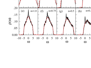
Figure 2: (Color online) Evolution of the DOS with doping for a $12\times 12$ lattice with $U=8t$, $W=12t$, $V=0$ and 1000-2000 impurity configurations. (a)-(d) Black solid lines and red dashed lines represent the results of LDMFT and effective medium calculations respectively. The Lorentz broadening is $\gamma=0.025$ throughout this work. (e)-(h) Corresponding plots for paramagnetic HFA calculations are shown for the same parameters and 1000 impurity configurations.

We begin our discussion with the case $V=0$. While it is not clear that a system can be experimentally realized in which the off-diagonal self-energy vanishes, this case is interesting because it provides a relatively simple illustration of the role of strong correlations. Throughout this section, strong correlation effects are identified by comparisons between the HFA (which neglects correlations) and LDMFT.

The DOS is calculated from the self-consistently determined Green’s function via

$$\rho(\omega)=-\frac{1}{N\pi}\sum_{i}\mbox{Im }G_{ii}(\omega)$$ (28)

where the rank-$N$ matrix ${\bf G}(\omega)$ is given by Eq. (4). The evolution of $\rho(\omega)$ with doping is shown for $V=0$ in Fig. 2. We have chosen $W=12t$, which corresponds to $W=1.5D$ where $D=8t$ is the bandwidth in the clean noninteracting limit. We have taken $U=8t$, which is large relative to $t$, but is much less than the critical $U_{c}\approx W$ at which the Mott transition takes place. For comparison, we have shown results for LDMFT and for the HI+CPA described in Sec. II.3. These two theories employ the same approximation for the interaction and differ only in how they treat disorder: nonlocal spatial correlations between impurity sites and the charge density are neglected in effective medium approximations and are treated exactly in LDMFT. The two methods give quantitatively similar results, except for the ZBA that emerges away from half filling in LDMFT but is absent in HI+CPA.

We note that the sign of the ZBA in Fig. 2 is positive. This is different from the usual case discussed in the literature, but is consistent with AA theory, where a negative ZBA comes from the exchange self-energy while the Hartree self-energy makes a weak positive correction to the DOS. Since the Hubbard interaction has a vanishing exchange self-energy, the expectation from mean-field theory is for a positive ZBA when $V=0$. This is illustrated by the numerical HFA calculations shown in Fig. 2(e)-(h).

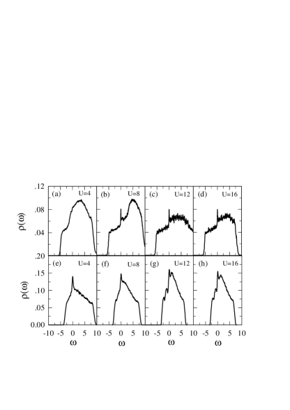
Figure 3: Evolution of the DOS with $U$ at quarter-filling for $W=12t$, $V=0$, and $8\times 8$ lattices with 1000 impurity configurations. The upper panels (a)-(d) show LDMFT results while the lower panels (e)-(h) show HFA results.

Although the sign of the ZBA is the same in LDMFT and HFA calculations, its magnitude is different. In particular, the peak at $\varepsilon_{F}$ is finite at all doping levels in the HFA but is absent near half-filling in the LDMFT calculations. This difference shows that strong correlations suppress the ZBA near half filling. Results for quarter filling are shown in Fig. 3 for a range of $U$, where it can be seen that the ZBA grows with $U$ when $U$ is small, but saturates when $U\gtrsim 8t$. A more technical discussion of these results is given in Sec. III.3, and we briefly summarize the main ideas of this discussion here.

The main distinction between weakly and strongly correlated systems is that the local charge density $n_{i}$ is a continuous variable in weakly correlated systems, but is restricted to near-integer values in strongly correlated systems. In the HFA, the energy of an isolated site is $\omega_{i}=\epsilon_{i}+Un_{i}/2$. For sites with $\varepsilon_{F}-U<\epsilon_{i}<\varepsilon_{F}$, the self-consistent equation for the charge density, $n_{i}=2f(\omega_{i})$ [where $f(x)$ is the Fermi function], will be satisfied at zero temperature by

$$\omega_{i}=\varepsilon_{F},\qquad n_{i}=2(\varepsilon_{F}-\epsilon_{i})/U,$$

where the second equality comes from rearranging the expression for $\omega_{i}$. Since a macroscopic fraction of sites satisfy $\varepsilon_{F}-U<\epsilon_{i}<\varepsilon_{F}$, a peak (i.e. a positive ZBA) is expected in the DOS at the Fermi energy in the atomic limit. Numerical calculations (not shown) find that the peak persists, but weakens, as $t/W$ grows.

In contrast, the poles in the spectral function for an isolated strongly correlated site are at $\omega_{i}=\epsilon_{i}$ and $\omega_{i}=\epsilon_{i}+U$. Because of the rigidity of the relationship between $\omega_{i}$ and $\epsilon_{i}$, the distribution of $\omega_{i}$ values follows the distribution of $\epsilon_{i}$ and a vanishing fraction of sites therefore have resonances at $\varepsilon_{F}$. There is, consequently, no ZBA when $t=0$; the ZBA in LDMFT calculations only occurs when $t/W$ is nonzero. The discussion in Sec. III.3 shows that the spectral weight in the ZBA is proportional to the hybridization function $\Lambda_{i}(\varepsilon_{F})$ between sites with $\epsilon_{i}\approx\varepsilon_{F}$ or $\epsilon_{i}+U\approx\varepsilon_{F}$ and the rest of the lattice. The absence of a ZBA at half-filling comes from the fact that these sites decouple from the lattice, i.e. $\Lambda_{i}(\varepsilon_{F})=0$, when $\varepsilon_{F}=U/2$.

Our analytical calculations in Sec. III.3 also suggest that $\Lambda_{i}(\varepsilon_{F})$ is a strong function of both $\varepsilon_{F}$ and $U$ provided $\varepsilon_{F}$ lies in the “central plateau” [by which we mean the broad peak in the DOS arising from the overlap of upper and lower Hubbard bands; see, for example, Fig. 2(a)]. Outside the central plateau, $\Lambda_{i}(\varepsilon_{F})$ is a weak function of both $\varepsilon_{F}$ and $U$. This is qualitatively consistent with the numerical results in Fig. 3, which show that the peak height increases with $U$ for $U\lesssim 8t$ and saturates at larger $U$: In the limit $t/W\rightarrow 0$, it is easy to show that $\varepsilon_{F}$ lies in the central plateau for $U<W/2$.

III.2 Numerical Results, $V\neq 0$

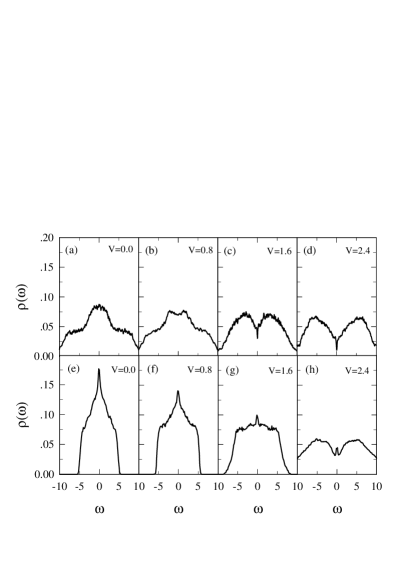
Figure 4: Evolution of the DOS with $V$ at half filling for $U=8t$ and $W=12t$. (a)-(d) LDMFT results for an $8\times 8$ lattice with 1000 impurity configurations. (e)-(h) HFA results are for the same parameters and $10\times 10$ lattices with 1000 impurity configurations.

We now consider the case $V\neq 0$. As for $V=0$, the influence of strong correlations is most visible at half filling. For the purposes of this discussion, the term “ES-like behavior” refers to a negative Hartree contribution to the DOS, and the term “AA-like behavior” refers to a Hartree contribution which is positive and an exchange contribution which is negative.

The DOS at half filling is shown in Fig. 4 for $U=8t$ and increasing $V$. In both the LDMFT and HFA results ES-like and AA-like behavior is present. As discussed in Vojta1998, there appears to be a transition as a function of energy, with ES-like behavior farther from the Fermi energy and AA-like behavior closer in. Following the arguments of ES,Efros and Shklovskii (1975) the average distance between states near the Fermi energy is very large. In our case the interaction has a finite range, and hence the ES behavior breaks down very near the Fermi energy. That the gap in Fig. 4 (d) is mostly ES-like, except right near the origin, can be seen in Fig. 5 (a) where the full result and a result with the Hartree term $V\sum_{j}n_{j}$ in Eq. 3 set to zero are compared. Note that the DOS does not satisfy the ES result $\rho(\omega)\propto|\omega-\varepsilon_{F}|$ because the interaction is short-range. The most striking difference between the LDMFT and HFA results is the more pronounced ES-like behavior in the strongly-correlated case. Strong correlations result in much less screening of the disorder than in the mean-field treatment, hence enhancing the disorder-driven ES-like behavior. That the AA-like behaviors in the LDMFT and HFA results differ in sign is not surprising given the very different treatment of $U$ in the two cases.

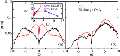
Figure 5: (color online) Contributions to the zero bias anomaly for $V=2.4t$ at (a) half filling and (b) quarter filling. For the curve labeled “Full”, both the exchange and Hartree self-energy contributions from the nearest neighbor interaction are retained, while for the curve labelled “Exchange Only”, the Hartree self-energy is set to zero. The curves show that the ZBA comes primarily from the Hartree contribution, and is therefore of the Efros-Shklovskii type. The inset shows results for the localization length at half-filling reproduced from a finite-size scaling analysis in Ref. Song et al., 2007 for $V=0$. The short localization length at large $U$ in LDMFT calculations, relative to HF calculations, is consistent with the enhanced Coulomb gap in the LDMFT calculations.

The results at quarter filling are shown in Fig. 6. The ZBA in the LDMFT results is less pronounced at quarter filling than at half filling. The narrow ZBA close to the Fermi energy crosses over from positive to negative, consistent with increasing $V$ and hence increasing negative exchange contribution of the AA type. As seen in Fig. 6(b), the Hartree self-energy modifies the DOS over a large energy range, but does not produce a gap-like feature at the Fermi energy. Exact studies of small clusters, to be reported elsewhere,Hongyi2009 suggest that the transition from large to small ZBA occurs when $\epsilon_{F}$ is shifted outside the central plateau described earlier. In the atomic limit, when $\epsilon_{F}$ lies within the central plateau $n_{i}$ may have three distinct values (0,1 or 2), whereas $n_{i}$ can only be 0 or 1 for $\epsilon_{F}$ below the lower edge of the plateau. In small clusters, this reduction in the range of possible charge states for individual sites directly results in a reduced ZBA. In marked contrast to the strongly-correlated results, the HFA results show an AA-like peak and an ES-like dip, both of which grow with increasing $V$.

Figure 7 shows the variation of the DOS with $U$ for $V=1.6t$. For the somewhat artificial case of $U=0$ shown in Fig. 6(a) and (e), the results differ slightly because the numerical HFA and LDMFT routines converge differently. Both obtain charge-density-wave order frustrated by the disorder, but with slightly shifted domain walls. In the HFA case, increasing $U$ screens the disorder, reducing the ES-like behavior. The AA-like Hartree peak is initially strengthened by $U$ but is reduced as the screening increases. At large $U$ [Fig. 7(h)], the DOS appraches the clean-limit result. In the LDMFT case, the screening produced by $U$ initially weakens the ES-like behavior. However, for larger values of $U$, the screening in the strongly correlated case is much less than that in mean field. The localization length based on a finite-size scaling analysis (calculated for $V=0$) is reproduced from a previous workSong et al. (2007) in the inset of Fig. 5. While the localization length grows monotonically with $U$ in the HFA, in the LDMFT it reaches a maximum at $U\approx 4t$ and decreases with increasing $U$ thereafter. Similarly, the ES-like behavior of the LDMFT DOS is initially weakened, but is not lost as in the HFA and saturates before the opening of the Mott gap.

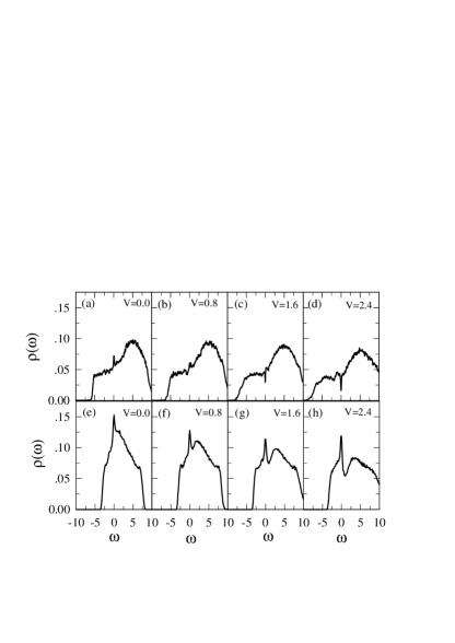
Figure 6: Evolution of the DOS with $V$ at quarter filling with $W=12t$ and $U=8t$. Calculations are for an $8\times 8$ site lattice with more than 1000 sample configurations for each parameter set. Results are shown for (a)-(d) LDFMT and (e)-(h) HFA.

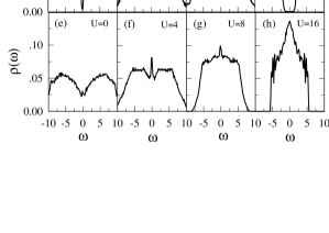
Figure 7: Evolution of the DOS with $U$ at half-filling with $W=12t$ and $V=1.6t$. (a)-(d) LDMFT and (e)-(h) HFA calculations are shown. Calculations are for an $8\times 8$ site lattice with more than 1000 sample configurations for each parameter set.

We note that, in Fig. 5, the exchange contribution to the ZBA depends only weakly on doping. We showed previously in Sec. II.2 that the exchange self-energy arising from the nonlocal interaction plays the same role as the exchange self-energy arising from a perturbative treatment of intraorbital interaction. Thus, the exchange-only curves shown in Fig. 5 should behave the same qualitatively as an exact treatment of the $V=0$ Anderson-Hubbard model. Such a study has been reported by Chiesa et al.,Chiesa2008 where the ZBA was found to be independent of doping for fillings $0.6\leq n\leq 1$. This is consistent with our findings.

When the Hartree self-energy is included, our findings differ substantially from Chiesa et al. In particular, the doping-dependence of the ZBA due to ES-like physics which we have reported here is not found when the interaction is purely local.Chiesa2008 We emphasize that the Hartree self-energy responsible for the ZBA is physically distinct from the exchange contributions arising from the Hubbard $U$ interaction, and can only occur when there is a finite-ranged interaction. In summary, the difference in results between Chiesa et al. and us appears to stem from the difference in the range of the electron-electron interactions.

III.3 Analysis of strong correlation effects on the zero bias anomaly

In this section, we discuss the origin of the ZBA in the $V=0$ case. We begin with Eq. (4) for the Green’s function. In the large disorder limit, it is possible to treat the hopping matrix element as a perturbation. When the matrix ${\bf t}$ is zero, ${\bf G}(\omega)$ decouples into a diagonal matrix describing an ensemble of isolated atoms with Green’s functions

$$G^{0}_{ii}(\omega)=\frac{1}{\omega-\epsilon_{i}-\Sigma^{0}_{ii}(\omega)},$$ (29)

where the superscript zeros refer to the isolated atomic systems and $\Sigma^{0}_{ii}(\omega)$ is given exactly by Eq. (7). The atomic Green’s function, $G^{0}_{ii}(\omega)$, has poles at

$$\omega^{0}_{i-}=\epsilon_{i};\quad\omega^{0}_{i+}=\epsilon_{i}+U,$$ (30)

with spectral weights

$$Z^{0}_{i-}=1-\frac{n_{i}}{2};\quad Z^{0}_{i+}=\frac{n_{i}}{2}.$$ (31)

The total density of states is found by averaging the imaginary part of $G^{0}_{ii}(\omega)$ over $\epsilon_{i}$ in the interval $-W/2<\epsilon_{i}<W/2$. Since the pole energies are linear functions of $\epsilon_{i}$, the total density of states is featureless at the Fermi energy.

Next, we use the fact that the diagonal matrix elements of Eq. (4) can be written in the form

$$G_{ii}(\omega)=\frac{1}{\omega-\epsilon_{i}-\Lambda_{i}(\omega)-\Sigma_{i}(\omega)},$$ (32)

where $\Lambda_{i}(\omega)$ is the hybridization function that describes the coupling of site $i$ to the rest of the lattice. It is

$$\Lambda_{i}(\omega) = \sum_{jk}t_{ij}t_{ki}G^{(i)}_{jk}(\omega)$$ (33)

$$\approx t^{2}\sum_{j}G^{0}_{jj}(\omega)$$

where $t_{ij}$ are the matrix elements of ${\bf t}$ between sites $i$ and $j$, $G^{(i)}_{jk}(\omega)$ is the Green’s function for the lattice with site $i$ removed, and the second line is the expansion of the first to $O(t^{2})$. Equation (33) applies formally to the limit that the localization length vanishes, but is qualitatively correct for $t\ll W$. We note that $\Lambda_{i}(\omega)$ is a complex function of frequency for metallic systems, but is real with a discrete spectrum of simple poles for Anderson-localized systems as we have here.

Recalling Eq. (7), we solve for the poles of $G_{ii}(\omega)$ to $O(t^{2})$:

$$\omega_{i-} = \epsilon_{i}+\left(1-\frac{n_{i}}{2}\right)\Lambda_{i}(\omega_{i-}),$$ (34a)

$$\omega_{i+} = \epsilon_{i}+U+\frac{n_{i}}{2}\Lambda_{i}(\omega_{i+}),$$ (34b)

where we have assumed $\Lambda_{i}\ll U$. In the approximation (33), $\Lambda_{i}(\omega_{i\pm})$ diverges when $\omega_{i\pm}$ is degenerate with any $\omega_{j\pm}$ for nearest neighbor site $j$. This is an artifact of the approximation since any degeneracy between $i$ and $j$ is lifted by hybridization of the orbitals. The poles of $\Lambda_{i}(\omega)$ must therefore differ from $\omega_{i\pm}$ by an energy $\gtrsim t$, and we impose a cutoff $|\Lambda_{i}(\omega_{i\pm})|<t$.

The spectral weights $Z_{i\pm}$ of the poles (34) are reduced by $O(t^{2})$ from $Z^{0}_{i\pm}$ and the remaining spectral weight appears at new poles resulting from hybridization of site $i$ with the rest of the lattice. These poles play a role in suppressing the ZBA in the limit that the localization length becomes large, but are of secondary importance when $t\ll W$ as in the current discussion.

Equations (34) contain the essential physics of the ZBA, which we summarize here before we go into the detailed calculations. In both equations, the local charge susceptibility $\chi_{ii}=-\partial n_{i}/\partial\epsilon_{i}$ is nonzero because of the hybridization function $\Lambda_{i}(\omega)$. The main idea is that, because $\chi_{ii}$ is nonzero, sites with energies $\epsilon_{i}$ that are sufficiently close to $\varepsilon_{F}$ ($\varepsilon_{F}-U$) can adjust their filling $n_{i}$ such that $\omega_{i-}=\varepsilon_{F}$ ($\omega_{i+}=\varepsilon_{F}$). The range of $\epsilon_{i}$ satisfying the criterion of “sufficiently close” is set by $\Lambda_{i}(\varepsilon_{F})$, and the weight under the ZBA peak is therefore also set by $\Lambda_{i}(\varepsilon_{F})$. The suppression of the ZBA at half filling then follows from the fact that the disorder average of $\Lambda_{i}(\varepsilon_{F})$ is an antisymmetric function of $\varepsilon_{F}$.

We consider sites with energies $\epsilon_{i}$ such that $\omega_{i\pm}=\varepsilon_{F}$. The expression for $\omega_{i\pm}$ requires knowledge of the charge density $n_{i}$, which is given by $n_{i}/2=\sum_{\pm}Z^{0}_{i\pm}f(\omega_{i\pm})+O(t^{2})$. For sites with $\omega_{i\pm}=\varepsilon_{F}$, this reduces to [excepting terms of $O(t^{2})$]

$$\frac{n_{i}}{2}=\left(1-\frac{n_{i}}{2}\right)f(\varepsilon_{F}),\quad(n_{i}<1)$$ (35)

for $\omega_{i-}=\varepsilon_{F}$ and

$$\frac{n_{i}}{2}=\left(1-\frac{n_{i}}{2}\right)+\frac{n_{i}}{2}f(\varepsilon_{F}),\quad(n_{i}>1)$$ (36)

for $\omega_{i+}=\varepsilon_{F}$. At zero temperature, $0<f(\varepsilon_{F})<1$ and these equations are satisfied for a range of $\epsilon_{i}$. Setting $\omega_{i-}=\varepsilon_{F}$ in Eq. (34a) and applying the restriction $0<n_{i}<1$, we generate the limits $\epsilon_{L}<\varepsilon_{F}-\epsilon_{i}<\epsilon_{U}$ on $\epsilon_{i}$, where

$$\epsilon_{L} = \min\left(\frac{\Lambda_{i}(\varepsilon_{F})}{2},\Lambda_{i}(\varepsilon_{F})\right),$$

$$\epsilon_{U} = \max\left(\frac{\Lambda_{i}(\varepsilon_{F})}{2},\Lambda_{i}(\varepsilon_{F})\right).$$

In this range [rearranging Eq. (34a)]

$$1-\frac{n_{i}}{2}=\frac{\varepsilon_{F}-\epsilon_{i}}{\Lambda_{i}(\varepsilon_{F})},$$ (37)

and the density of states at $\varepsilon_{F}$ coming from sites with $\omega_{i-}=\varepsilon_{F}$ is therefore

$$\delta\rho_{-}(\omega\approx\varepsilon_{F}) = \frac{1}{W}\int_{\varepsilon_{F}-\epsilon_{U}}^{\varepsilon_{F}-\epsilon_{L}}d\epsilon_{i}Z_{i-}\delta(\omega-\varepsilon_{F})$$ (38)

$$= \frac{3}{8}\frac{|\Lambda(\varepsilon_{F})|}{W}\delta(\omega-\varepsilon_{F})+O(t^{4}).$$

In this equation, $|\Lambda(\varepsilon_{F})|$ is an average over $|\Lambda_{i}(\varepsilon_{F})|$. An identical result can be found for sites with resonance energies $\omega_{i+}=\varepsilon_{F}$, so that the total density of states near the Fermi energy is

$$\rho(\omega\approx\varepsilon_{F})=\frac{3}{4}\frac{|\Lambda(\varepsilon_{F})|}{W}\delta(\omega-\varepsilon_{F}).$$ (39)

Equation (39) shows that the ZBA is a delta-function at zero temperature. At finite temperatures $T$, the ZBA is a peak of width $\sim T$. The spectral weight in the peak is proportional to the hybridization function $\Lambda(\varepsilon_{F})$, and we next show how this depends on doping.

We consider a site $i$ in a lattice with coordination number $Z_{c}$, whose nearest neighbors have randomly chosen site energies. At half filling ($\varepsilon_{F}=U/2$), the terms $G_{jj}^{0}(\varepsilon_{F})$ in the sum in (33) are positive or negative with equal probability, and tend to cancel. As the filling is reduced, the probability that $G_{jj}^{0}(\varepsilon_{F})$ is negative (positive) becomes larger (smaller). We make a rough calculation that illustrates this behavior by replacing the sum over site index $j$ in (33) with an integral over $\epsilon_{j}$. Thus

$$\Lambda_{i}(\varepsilon_{F}) \approx \frac{t^{2}Z_{c}}{W}\int_{-W/2}^{W/2}d\epsilon\left(\frac{1-n_{\epsilon}/2}{\varepsilon_{F}-\epsilon}+\frac{n_{\epsilon}/2}{\varepsilon_{F}-\epsilon-U}\right),$$

where $n_{\epsilon}$ is the charge density for sites with site-energy $\epsilon$. Recalling our constraint $|\Lambda_{i}(\varepsilon_{F})|\lesssim t$, we introduce cutoffs near the poles of the integrand. Noting that

$$n_{\epsilon}=\left\{\begin{array}[]{ll}2,&\epsilon<\varepsilon_{F}-U\\ 1,&\varepsilon_{F}-U<\epsilon<\varepsilon_{F}\\ 0,&\epsilon>\varepsilon_{F}\end{array}\right.$$

we get

$$\Lambda_{i}(\varepsilon_{F})\approx\frac{t^{2}Z_{c}}{W}\ln\left(\frac{\frac{W}{2}+\varepsilon_{F}-U}{\frac{W}{2}-\varepsilon_{F}}\right),$$ (40a)

for $$U-\frac{W}{2}<\varepsilon_{F}<\frac{W}{2}$$ and

$$\Lambda_{i}(\varepsilon_{F}) \approx \frac{t^{2}Z_{c}}{W}\left[\ln\left(\frac{\frac{W}{2}+\varepsilon_{F}}{\frac{W}{2}-\varepsilon_{F}}\right)\right.+\frac{1}{2}\ln\left(\frac{U-\frac{W}{2}-\varepsilon_{F}}{\frac{W}{2}+\varepsilon_{F}}\right)$$ (40b)

$$\left.+\frac{1}{2}\ln\left(\frac{t}{U}\right)\right]$$

for $-\frac{W}{2}<\varepsilon_{F}<U-\frac{W}{2}$. The logarithmic divergences in Eqs. (40) are artificial and must be cut off whenever any numerator or denominator has a magnitude smaller than $t$. Equation (40a) applies when the Fermi level sits in the central plateau, and shows that $\Lambda_{i}(\varepsilon_{F})$ is antisymmetric about half-filling (i.e. $\varepsilon_{F}=U/2$), and grows linearly away from half-filling. Outside of the central plateau, $\Lambda_{i}(\varepsilon_{F})$ is a weak function of $\varepsilon_{F}$.

In order to compare with Fig. 3, we evaluate Eq. (40b) at quarter filling, which for small $t$ corresponds to

$$\varepsilon_{F}\approx\left\{\begin{array}[]{ll}\frac{U}{2}-\frac{W}{4},&U<\frac{W}{2}\\ 0,&U>\frac{W}{2}\end{array}\right.$$

Then Eq. (40b) gives

$$|\Lambda_{i}(\varepsilon_{F})|\approx\frac{t^{2}Z_{c}}{W}\left[\ln\left(\frac{\sqrt{(\frac{W}{2})^{2}-U^{2}}}{\frac{3}{2}W-U}\right)-\frac{1}{2}\ln\left(\frac{U}{t}\right)\right],$$ (41a)

for $$U<\frac{W}{2}$$, and

$$|\Lambda_{i}(\varepsilon_{F})|\approx\frac{t^{2}Z_{c}}{2W}\left[\ln\left(\frac{2U-W}{W}\right)-\ln\left(\frac{U}{t}\right)\right],$$ (41b)

for $U>\frac{W}{2}$. In Eqs. (41b), $|\Lambda_{i}(\varepsilon_{F})|$ grows linearly with $U$ for small $U$ (recall that there is a cutoff such that $\ln(U/t)\rightarrow\ln(t/t)$ when $U<t$), and saturates at a finite value when $U\gg\frac{W}{2}$. Both these results, and the results at half filling in Eq. (40a) are qualitatively consistent with the numerical results shown in Figs. 2 and 3.

IV Conclusions

We have studied the effects of strong correlations on the zero bias anomaly in the density of states for disordered interacting systems. Our results show significant doping dependence. When only local interactions are included, a positive ZBA is suppressed by strong correlations at half filling due to cancelation in the hybridization function responsible for the peak. When nearest-neighbor interactions are included (simultaneously producing a more accurate treatment of the Hubbard $U$ term), strong correlations modify the mean field results at both half and quarter filling. In particular, at half filling ES-like behavior is enhanced due to reduced screening in the strongly correlated system, whereas at quarter filling the ZBA is smaller reflecting the doping dependence of the ES physics.

References

- Efros and Shklovskii (1975) A. L. Efros and B. I. Shklovskii, J. Phys. C: Solid State Phys. 8, L49 (1975).
- Efros (1976) A. L. Efros, J. Phys. C: Solid State Phys. 9, 2021 (1976).
- Altshuler and Aronov (1985) B. L. Altshuler and A. G. Aronov, Electron-Electron Interactions in Disordered Systems, vol. 10 of Modern Problems in Condensed Matter Sciences (North-Holland, 1985).
- Butko, DiTusa, and Adams (2000) V. Y. Butko, J. F. DiTusa and P. W. Adams, Phys. Rev. Lett. 84, 1543 (2000).
- Dagotto (1994) E. Dagotto, Rev. Mod. Phys. 66, 763 (1994).
- Imada et al. (1998) M. Imada, A. Fujimori, and Y. Tokura, Rev. Mod. Phys. 70, 1039 (1998).
- (7) F. J. Morin, Phys. Rev. Lett. 3, 34 (1959).
- Hanasaki et al. (2006) N. Hanasaki, M. Kinuhara, I. Kezsmarki, S. Iguchi, S. Miyasaka, N. Takeshita, C. Terakura, H. Takagi, and Y. Tokura, Phys. Rev. Lett. 96, 116403 (2006).
- Sarma et al. (1998) D. D. Sarma, A. Chainani, S. R. Krishnakumar, E. Vescovo, C. Carbone, W. Eberhardt, O. Rader, C. Jung, C. Hellwig, W. Gudat, et al., Phys. Rev. Lett. 80, 4004 (1998).
- Ino et al. (2004) A. Ino, T. Okane, S.-I. Fujimori, A. Fujimori, T. Mizokawa, Y. Yasui, T. Nishikawa, and M. Sato, Phys. Rev. B 69, 195116 (2004).
- Kim et al. (2006) J. Kim, J. Kim, B. G. Park, and S. J. Oh, Phys. Rev. B 73, 235109 (2006).
- Nakatsuji et al. (2004) S. Nakatsuji, V. Dobrosavljevic, D. Tanaskovic, M. Minakata, H. Fukazawa, and Y. Maeno, Phys. Rev. Lett. 93, 146401 (2004).
- Kim et al. (2005) K. W. Kim, J. S. Lee, T. W. Noh, S. R. Lee, and K. Char, Phys. Rev. B 71, 125104 (2005).
- (14) A notable recent exception is Ref. Chiesa2008, .
- (15) S. Chiesa, P. B. Chakraborty, W. E. Pickett, and R. T. Scalettar, arxiv:0804.4463.
- (16) M. Milovanović, S. Sachdev, and R. N. Bhatt, Phys. Rev. Lett. 63, 82 (1989).
- (17) M. A. Tusch and D. E. Logan, Phys. Rev. B 48, 14843 (1993).
- (18) D. Heidarian and N. Trivedi, Phys. Rev. Lett. 93, 126401 (2004).
- Fazileh, Gooding, Atkinson, and Johnson (2006) F. Fazileh, R. J. Gooding W. A. Atkinson and D. C. Johnson, Phys. Rev. Lett. 96, 046410 (2006).
- Ulmke et al. (1995) M. Ulmke, V. Janis̆, and D. Vollhardt, Phys. Rev. B (1995).
- Laad et al. (2001) M. S. Laad, L. Craco, and E. Müller-Hartmann, Phys. Rev. B 64, 195114 (2001).
- Dobrosavljević et al. (2003) V. Dobrosavljević, A. A. Pastor, and B. K. Nikolić, Europhys. Lett. 62, 76 (2003).
- Byczuk et al. (2005) K. Byczuk, W. Hofstetter, and D. Vollhardt, Phys. Rev. Lett. 94, 056404 (2005).
- Balzer and Potthoff (2005) M. Balzer and M. Potthoff, Physica B 359-361, 768 (2005).
- Lombardo et al. (2006) P. Lombardo, R. Hayn, and G. I. Japaridze, Phys. Rev. B 74, 085116 (2006).
- Dobrosavljević and Kotliar (1997) V. Dobrosavljević and G. Kotliar, Phys. Rev. Lett. 78, 3943 (1997).
- Miranda and Dobrosavljević (2005) E. Miranda and V. Dobrosavljević, Rep. Prog. Phys. 68, 2337 (2005).
- Song et al. (2007) Y. Song, R. Wortis, and W. A. Atkinson, Phys. Rev. B. 77, 054202 (2008).
- (29) Elliott H. Lieb and F. Y. Wu, Phys. Rev. Lett. 20, 1445 (1968).
- (30) J. E. Hirsch, Phys. Rev. B 31, 4403 (1985).
- (31) S. R. White, D. J. Scalapino, R. L. Sugar, E. Y. Loh, J. E. Gubernatis, and R. T. Scalettar, Phys. Rev. B 40, 506 (1989).
- (32) Y. Otsuka and Y. Hatsugai, J. Phys. Cond. Mat. 12, 9317 (2000)
- (33) Similar real-space formalisms have been employed by others to describe heterostructures, notably J. K. Freericks, Phys. Rev. B 70, 195342 (2004); S. Okamoto and A. J. Millis, Phys. Rev. B 70, 241104 (2004); W.-C. Lee and A. H. MacDonald, Phys. Rev. B 74, 075106 (2006); S. Yunoki, A. Moreo, E. Dagotto, S. Okamoto, S. S. Kancharla, and A. Fujimori, Phys. Rev. B 76, 064532 (2007). A similar formalism has also been applied to the disordered Bethe lattice in Refs. Dobrosavljević and Kotliar, 1997; Miranda and Dobrosavljević, 2005 where it was termed “statistical DMFT”.
- (34) A. Georges, G. Kotliar, W. Krauth, and M. J. Rozenberg, Rev. Mod. Phys. 68, 13 (1996).
- (35) Note that in cases where the self-energy can be expressed analytically in terms of or in terms of expectation values derived from , it is possible to eliminate the step of explicitly constructing the Anderson impurity problem. This presents a considerable simplification and in the current case reduces the problem to one which is equivalent to solving a combination of Hartree-Fock and Hubbard-I equations in real space on a disordered lattice.
- (36) P. Fulde Electron Correlations in Molecules and Solids, vol. 100 of Springer Series in Solid State Sciences (Springer, 1995).
- (37) B. Mehlig, H. Eskes, R. Hayn, and M. B. J. Meinders, Phys. Rev. B 52, 2463 (1995).
- (38) C. Grober, R. Eder, and W. Hanke, Phys. Rev. B 62, 4336 (2000).
- (39) F. Mancini and A. Avella, Adv. in Phys. 53, 537 (2004).
- (40) Frank Epperlein, Michael Schreiber, and Thomas Vojta, Phys. Rev. B 56, 5890 (1997).
- (41) Hongyi Chen, R. Wortis, and W. A. Atkinson (unpublished).