Three- and four-state rock-paper-scissors games with diffusion

Abstract

Cyclic dominance of three species is a commonly occurring interaction dynamics, often denoted the rock-paper-scissors (RPS) game. Such type of interactions is known to promote species coexistence. Here, we generalize recent results of Reichenbach et al. (e.g. Nature 448, 1046 (2007)) of a four-state variant of RPS. We show that spiral formation takes place only without a conservation law for the total density. Nevertheless, in general fast diffusion can destroy species coexistence. We also generalize the four-state model to slightly varying reaction rates. This is shown both analytically and numerically not to change pattern formation, or the effective wave length of the spirals, and therefore does not alter the qualitative properties of the cross-over to extinction.

I Introduction

Pattern formation and stability of ecological multi-species systems have attained a lot of interest recently aranson2002 ; zhdanov2002 ; sole06 ; kerr2002 ; reichenbach2007 . These two topics are usually linked together by the well-known fact that spatial inhomogeneity can stabilize species co-existence sole06 ; briggs04 , and understanding both the issues themselves and their connection is of great importance.

An important class of model systems here are the so-called rock-paper-scissors games. They describe the dynamics of three species that cyclically dominate each other szabo1999 ; szabo2004 ; szolnoki2004b ; reichenbach2006 ; claussen2008 . Typically, these systems involve a conservation law for the total density. This can be imposed by writing rate equations such that the densities of the three species always sum up to unity, or employing lattice-based simulations where a site is always in exactly one of the three states. In this case, the system has a reactive fixed point which can be unstable, marginally stable, or stable depending on other properties of the particular setting, such as discreteness of the populations or dimensionality. There is a large body of work on very similar models with different microscopic update rules szabo2002 ; szolnoki2004 ; szolnoki2005 ; nishiuchi2008 , and recently more complicated six-species systems with a similar conservation law have been studied szabo2008 . Several rock-paper-scissors–like processes have been identified in ecology, both spatial kerr2002 ; keymer2006 ; loose2008 and non-spatial sinervo1996 ; kirkup2004 , as well as in other contexts not related to population dynamics such as the public goods game semmann2003 .

Recently, Reichenbach and co-workers have studied a version of the rock-paper-scissors game in which the conservation law has been removed reichenbach2007 ; reichenbach2008 . In lattice simulations, this is achieved by building the model on four states: the three original cyclically dominating states and a fourth one that denotes empty space. If diffusion is added, it does not interfere with the global conservation laws or absence thereof, but serves to set a length scale different from that set by the lattice constant. It has been shown that in this case the reactive fixed point is always unstable, and with diffusion in two dimensions spiral patterns form, similar to those in the complex Ginzburg-Landau equation (CGLE) aranson2002 , or vortices in ecological systems tainaka1989 ; tainaka1994 . The main conclusion in Refs. reichenbach2007 ; reichenbach2008 has been that as a function of the diffusion constant $D$ there is a cross-over from a reactive state with all three populations present to an absorbing state in which only one of the populations survives. This is argued to take place when the value of the diffusion constant is such that the spirals outgrow the system size.

Here we analyze these models further by considering both the four-state case and a three-state version with a conservation of the total density. We show that removing the conservation law gives rise to spiral formation that does not occur if the total density is conserved. However, in spite of this, there is a mechanism involving a diffusion-induced length scale that leads to a cross-over to an absorbing state. Therefore, conclusions regarding population stability are qualitatively the same for both cases. Second, all previous theoretical studies have assumed that the microscopic processes are rate-symmetric. In other words, one can cyclically permute the three populations without any change whatsoever. However, experiments can both explicitly show formation of spiral patterns kerr2002 and still be built such that the detailed pair-wise reaction mechanisms are qualitatively different for different pairs of species loose2008 . It is apparent that a small rate-asymmetry does not change these properties. We introduce rate-asymmetry into the four-state model reichenbach2007 , and argue analytically, that the resulting system is still essentially the CGLE but only after an unimportant (in the first order) change of variables. This result, also confirmed by direct simulations, shows that already rate-symmetric theory and rate-asymmetric experiments are comparable.

This paper is structured as follows. In Section II, we define both the three- and the four-state models with and without diffusion, and discuss in more detail what is previously known about them. In Section III, we present our results for all cases considered. Finally, Section IV ends the paper with a summary and discussion.

II The models and earlier work

The three-state RPS model describes cyclic dominance of three states, $A$, $B$, and $C$, and is defined by the following reaction equations and corresponding rates

$$\begin{array}[]{ccccc}AB&\rightarrow&AA&\mathrm{with}\;\mathrm{rate}&\mu\\ BC&\rightarrow&BB&\mathrm{with}\;\mathrm{rate}&\mu\\ CA&\rightarrow&CC&\mathrm{with}\;\mathrm{rate}&\mu\,.\end{array}$$ (1)

In the mean-field approximation, the rate equations describing the evolution of the system are

$$\begin{array}[]{ccc}\partial_{t}a&=&\mu ab-\mu ac\\ \partial_{t}b&=&\mu bc-\mu ab\\ \partial_{t}c&=&\mu ca-\mu cb\,,\end{array}$$ (2)

where $a$, $b$, and $c$ are densities of the states $A$, $B$, and $C$, respectively. The rate equations have a reactive fixed point at $a=b=c=\frac{1}{3}$, which is known to be marginally stable. Such behavior is usually considered highly unrealistic in biologically motivated systems, and therefore the MF approximation of this system is considered to be of no relevance.

The same model with discrete densities (i.e. finite populations) with noise has been studied in the mean-field like, non-spatial version reichenbach2006 . In this case, the marginal stability of the fixed point remains, and the behavior of the system becomes a random walk in the space of marginally stable circular trajectories. Since the population is finite, this always leads to extinction in the infinite-time limit.

However, in two-dimensional spatially extended systems the three-state RPS game is known to be stable, at least in large enough systems. The simplest known theoretical approach reproducing the behavior is the four-site approximation by Szabo and co-workers szabo2004 .

In empirical systems, the three states above are often considered to be three cyclically dominating strains of bacteria. In such settings, the dominance of strain $A$ over strain $B$ leads microscopically to deaths of individuals of strain $B$. In these cases, strain $A$ does not reproduce immediately but non-occupied space is created, and the filling-in via reproduction of any strain is a separate process. Therefore, the following set of reaction equations has been proposed reichenbach2007

$$\begin{array}[]{ccccc}AB&\rightarrow&EA&\mathrm{with}\;\mathrm{rate}&\sigma\\ BC&\rightarrow&EB&\mathrm{with}\;\mathrm{rate}&\sigma\\ CA&\rightarrow&EC&\mathrm{with}\;\mathrm{rate}&\sigma\\ XE&\rightarrow&XX&\mathrm{with}\;\mathrm{rate}&\mu\,,\end{array}$$ (3)

where $X$ can refer to any state and $E$ denotes empty space. In contrast to Eqs. (1) in which the only parameter $\mu$ sets the time scale, these reaction equations contain two independent parameters. The corresponding rate equations are reichenbach2008

$$\begin{array}[]{ccc}\partial_{t}a&=&a[\mu(1-\rho)-\sigma c]\\ \partial_{t}b&=&b[\mu(1-\rho)-\sigma a]\\ \partial_{t}c&=&c[\mu(1-\rho)-\sigma b]\,,\end{array}$$ (4)

where $\rho=a+b+c$ is the total density. These equations have a reactive fixed point

$$a=b=c=\frac{\mu}{3\mu+\sigma}\,,$$ (5)

which is linearly unstable for all $\mu$ and $\sigma$ reichenbach2008 .

To generalize both models to their spatially extended versions, let the populations live on regular square lattices, the reactions take place only in nearest-neighbour contact, and amend the reaction equations with an exchange reaction

$$XY\rightarrow YX\;\;\mathrm{with}\;\;\mathrm{rate}\;\;D\,,$$ (6)

where $X$ and $Y$ can denote any state (including empty space in the four-state model), and $D$ is the diffusion constant.

Exploiting the instability of the fixed point of Eq. (5) a spatially extended version of the system has been recently approximatively mapped reichenbach2008 to the complex Ginzburg-Landau equation (CGLE) aranson2002 . In the mapping, one shifts the reactive fixed point to the origin, expands around it to find a two-dimensional invariant manifold of the dynamics, expresses the dynamics on the manifold, and performs a normal-form transformation, i.e. finds the quadratic transformation that is an identity mapping to first order and the result of which has no quadratic terms. Upon adding the diffusion according to Eq. (6), one arrives at a variant of the CGLE.

In accordance with the known behavior of the CGLE, it has been found that the spatial four-state model with diffusion leads to formation of spirals reichenbach2007 . They have a characteristic wave length that scales as the square root of the diffusion constant. When the wave length is of the order of the system size, there is essentially one spiral in the system. With even larger diffusion constants, the system behaves essentially as a completely coupled one and an extinction due to similar reasons as in the noisy non-spatial case takes place reichenbach2006 . In other words, there is an absorbing-state cross-over as a function of the diffusion constant $D$ when the spiral wave length reaches the system size.

In direct numerical simulations, all variants of the model are simulated on a regular square lattice of size $L\times L$. For each microscopic time step, a process (selection or diffusion in the three-state case; selection, reproduction, or diffusion in the four-state case) is chosen randomly with probabilities proportional to the rates, a random lattice site and its random neighbour are chosen uniformly at random, and the reaction is executed if allowed by the rules. The time is increased by $\Delta t=1/(\tau L^{2})$ where $\tau$ is the sum of the rates for each case. The procedure is repeated until the time $t$ reaches a predefined value.

III Results

III.1 Three-state model

III.1.1 Mapping to the CGLE

To answer the question if explicit handling of empty space, i.e. using the four-state model instead of the more traditional three-state one, is really necessary to see the spiral pattern formation and the consequent absorbing-state cross-over, we map the three-state model to an equation resembling the CGLE as closely as possible. To start, set the timescale in Eqs. (2) by choosing $\mu=1$. Introduce new variables $x_{A}=a-\frac{1}{3}$, $x_{B}=b-\frac{1}{3}$, $x_{C}=c-\frac{1}{3}$, and use the conservation of the total density $a+b+c=1$ to express the dynamics in terms of $x_{A}$ and $x_{B}$ as follows

$$\partial_{t}x_{A}=\frac{1}{3}x_{A}+\frac{2}{3}x_{B}+x_{A}^{2}+2x_{A}x_{B}$$ (7)

$$\partial_{t}x_{B}=-\frac{2}{3}x_{A}-\frac{1}{3}x_{B}-2x_{A}x_{B}-x_{B}^{2}\,.$$ (8)

Note that the treatment here differs from that of the four-state model, since there is no need to reduce the number of dynamical variables by finding an invariant manifold. From Eq. (7), the linearization of the system around the fixed point is

$$\partial_{t}\left(\begin{array}[]{c}x_{A}\\ x_{B}\end{array}\right)=\left(\begin{array}[]{cc}\frac{1}{3}&\frac{2}{3}\\ -\frac{2}{3}&-\frac{1}{3}\end{array}\right)\left(\begin{array}[]{c}x_{A}\\ x_{B}\end{array}\right)\,.$$ (9)

The eigenvalues of the linearization matrix are

$$\lambda=\pm i\frac{\sqrt{3}}{3}\,,$$ (10)

which recovers the known fact that the fixed point is marginally stable.

To transform Eqs. (7) to a normal form, apply first the change of variables

$$y_{A}=\frac{2}{\sqrt{3}}x_{A}+\frac{1}{\sqrt{3}}x_{B}$$ (11)

$$y_{B}=x_{B}$$ (12)

to arrive at the rate equations, now expressed in terms of $y_{A}$ and $y_{B}$

$$\partial_{t}y_{A}=\frac{\sqrt{3}}{3}y_{B}+\frac{\sqrt{3}}{2}(y_{A}^{2}-y_{B}^{2})$$ (13)

$$\partial_{t}y_{B}=-\frac{\sqrt{3}}{3}y_{A}-\sqrt{3}y_{A}y_{B}\,.$$ (14)

The reason for this particular change of variables will become clear when comparing the normal form to be calculated below to the CGLE. Namely, this transformation ensures that the linear terms are written in a directly comparable way.

Now, let us turn Eqs. (13) into their normal form. Here, the task is to find such a quadratic transformation from the variables $y_{A}$ and $y_{B}$ to a new pair of variables, say $z_{A}$ and $z_{B}$ such that the $y$’s and the $z$’s coincide to linear order and that the rate equations for $z$ do not contain quadratic terms. In general, finding such a transformation involves finding the inverse of a particular $6\times 6$ matrix, and particular corner cases of singular matrices could cause the transform not to exist. However, in the present example, this does not happen.

By imposing the restrictions above, we find the necessary transformation to be the following

$$z_{A}=y_{A}+y_{A}y_{B}$$ (15)

$$z_{B}=y_{B}+\frac{1}{2}y_{A}^{2}-\frac{1}{2}y_{B}^{2}$$ (16)

and the resulting normal form

$$\partial_{t}z_{A}=\omega z_{B}+c_{2}z_{A}^{2}z_{B}+c_{2}z_{B}^{3}$$ (17)

$$\partial_{t}z_{B}=-\omega z_{A}-c_{2}z_{A}^{3}-c_{2}z_{A}z_{B}^{2}\,,$$ (18)

where $\omega=\frac{\sqrt{3}}{3}$ and $c_{2}=-\frac{\sqrt{3}}{2}$ with fourth-order and higher terms in $y_{A}$ and $y_{B}$ omitted. To connect this to the CGLE, consider the complex variable $z=z_{A}+iz_{B}$. Now, Eqs. (17) with added diffusion can be cast as

$$\partial_{t}z=i\omega z+D\Delta z+ic_{2}|z|^{2}z\,.$$ (19)

Further, changing to a rotating coordinate system (replace $z$ by $ze^{i\omega t}$) removes the purely imaginary linear term, and the resulting equation reads

$$\partial_{t}z=D\Delta z+ic_{2}|z|^{2}z\,,$$ (20)

which is already close to the standard form of the CGLE

$$\partial_{t}z=z+(1+ib)\Delta z-(1+ic)|z|^{2}z\,.$$ (21)

Comparing Eqs. (20) and (21) reveals a crucial difference: in the CGLE there is a non-zero linear term whereas in the normal-form complex PDE the three-state model maps to, there is none. This is a direct consequence of the stability properties of the original MF equations.

To further argue why omitting the linear term matters, consider a variant of the CGLE with a more general linear term $\nu z$

$$\partial_{\tilde{t}}\tilde{z}=\nu\tilde{z}+(1+ib)\tilde{\Delta}\tilde{z}-(1+ic)|\tilde{z}|^{2}\tilde{z}\,.$$ (22)

Given $\nu>0$, Eq. (21) is recovered after the scalings $\tilde{z}=\sqrt{\nu}z$, $\tilde{t}=1/\nu t$, and $x=\sqrt{\nu}\tilde{x}$ aranson2002 . Substitute a generic single-spiral solution aranson2002

$$z=a(r)e^{i(\omega t\pm\phi+\psi(r))}\,,$$ (23)

where $a(r)$ and $\psi(r)$ are real functions and $r$ and $\phi$ are the spatial coordinates in the cylindrical coordinate system, with the spiral core at the origin, to Eq. (22). Consider the limit $r\to\infty$ assuming that $a(r)$ tends to a constant (i.e. the solutions are bounded) and that $\psi(r)$ tends to $qr$, i.e. asymptotically the spiral looks like a plane wave with wave number $q$. One finds that for the single-spiral solution to exist, the equality

$$a(r)\to a_{0}=\sqrt{\nu-q^{2}}$$ (24)

has to hold. Since $a(r)$ is real, spiral solutions with a finite wave length exist only for positive $\nu$. In other words, there are no spiral solutions in the three-state RPS game. The same argument can be repeated for plane waves as well, leading to exactly the same condition.

We have also verified the conclusion by direct numerical simulations of the three-state model. Example configurations are plotted in Fig. 1 in panels (d), (e), and (f). There are indeed no signs of spiral formation, but a growing diffusion constant does change the spatial correlations in the system. Below, we show that this leads to an absorbing-state cross-over as a function of the diffusion constant regardless of the absence of spiral pattern formation.

Figure 1: (Color online) Example runs of the system in a lattice of size $L\times L=200$. (a), (b) and (c): the four-state model with different diffusion constants and $\mu=\sigma=1$. (d), (e), (f): the three-state model with different diffusion constants and $\mu=1$. (g), (h), (i): the rate-asymmetric four-state model with different asymmetries $r=1+\epsilon$, $D=\mu=\sigma=1.0$.

III.1.2 Extinction cross-over

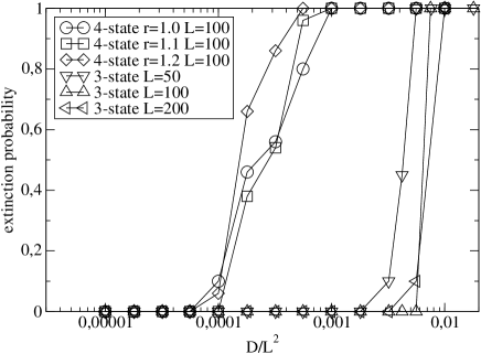
Both the three-state and the four-state models have an emergent length scale in the diffusive regime. In the four-state model, this is the spiral wave length, and in the three-state case it is simply the correlation length. Since the four-state model has an extinction cross-over as a function of the diffusion constant because of the length scale, it is natural to suspect that this is the case in the three-state model as well. We have performed extensive numerical simulations of both models to study the extinction probability as a function of the diffusion constants. The results are shown in Fig. 2. For the four-state model we recover the results of Ref. reichenbach2007 and the results for the three-state model show a similar cross-over. In both cases, the diffusion constant at the cross-over scales as $D_{c}\sim L^{2}$ where $L$ is the linear dimension of the lattice.

Figure 2: The extinction probability as a function of the scaled diffusion constant $D/L^{2}$ in various cases. For both the three- and the four-state model there is a cross-over to an absorbing state with two of the three subpopulations extinct. The location of this cross-over scales as $D_{c}\propto L^{2}$ in both cases and in the four-state case the introduction of rate-asymmetry does not affect the location of the cross-over for small asymmetries.

Next, we argue that the extinction cross-over is caused by the presence of a correlation length, applying an argument previously used in the context of the contact process with diffusion marro1999 ; dantas2007 ; messer2008 . Imagine the system in its steady-state, with a small spatially localized perturbation caused by noise. Due to the exchange reactions, this perturbation diffuses with diffusion constant $2D$, where the factor of two comes from the fact that at each exchange reaction two particles moved. If the typical lifetime of such a perturbation is $t_{d}$, it will diffuse up to distance $x=\sqrt{2Dt_{d}}$ before decaying. After estimating $t_{d}$, the cross-over should take place when $L^{2}=2Dt_{d}$ so that the properly scaled diffusion constant at the cross-over becomes

$$\frac{D}{L^{2}}=\frac{1}{2t_{d}}\ .$$ (25)

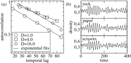
To estimate the perturbation lifetime, we have computed the autocorrelation function of the time series of the densities. Fig. 3 shows the autocorrelation for several diffusion constants $D$ and a corresponding time series. The immediate observations are that the autocorrelation function is independent of $D$ and that it decays exponentially so that a well-defined timescale exists. From the linear fits, we can extract the time scale and we have found $t_{d}\approx 66$ (see Sec. II for the definition of unit of time in the simulations), from which we get that at the cross-over we have $\frac{D}{L^{2}}\approx 7.6\cdot 10^{-3}$. This estimate corresponds well to the location of the cross-over in Fig. 2.

Figure 3: (a) The envelope of the autocorrelation function of the density of state $A$ in the three-state model with different diffusion constants $D$. The symbols show the numerical results and the solid black lines are fits to the form $a(t)\propto e^{-t/t_{d}}$. For a wide range of diffusion constants we find $t_{d}=66$ independent of $D$. (b) The corresponding time series of the densities of the three states show oscillations with wildly fluctuating amplitudes, often associated with almost-unstable dynamics and time-scale separation peltomaki2008 . The parameters are $L=200$ and $\mu=1.0$.

III.2 Four-state model

The previous formulations of both the three- and the four-state models have assumed invariance of the model under cyclic permutations of the three non-empty states. In particular, this is seen in the rate equations (2) and (4) where the reproduction rate $\mu$ is the same for all species. However, this assumption is not necessarily fulfilled by any realistic empirical scenario loose2008 . To find out if this matters, we define a rate-asymmetric variant of the four-state model by the following reaction equations

$$\begin{array}[]{ccccc}AB&\rightarrow&AE&\mathrm{with}\;\mathrm{rate}&\sigma\\ BC&\rightarrow&BE&\mathrm{with}\;\mathrm{rate}&\sigma\\ CA&\rightarrow&CE&\mathrm{with}\;\mathrm{rate}&\sigma\\ AE&\rightarrow&AA&\mathrm{with}\;\mathrm{rate}&\mu\\ BE&\rightarrow&BB&\mathrm{with}\;\mathrm{rate}&\mu\\ CE&\rightarrow&CC&\mathrm{with}\;\mathrm{rate}&r\mu\\ XY&\rightarrow&YX&\mathrm{with}\;\mathrm{rate}&D\,,\end{array}$$ (26)

where $r=1+\epsilon$ ($\epsilon>0$) is assumed to be close to unity, i.e. $\epsilon\ll 1$, and $X$ and $Y$ can refer to any state (including the empty state $E$). This is the simplest possible extension of the original four-state model that incorporates rate-asymmetry. The corresponding MF rate equations are

$$\begin{array}[]{ccc}\partial_{t}a&=&a[\mu(1-\rho)-\sigma c]\\ \partial_{t}b&=&b[\mu(1-\rho)-\sigma a]\\ \partial_{t}c&=&c[r\mu(1-\rho)-\sigma b]\,.\end{array}$$ (27)

These have the reactive fixed point

$$a=c=\frac{\mu}{(2+r)\mu+\sigma}\,;\,b=\frac{r\mu}{(2+r)\mu+\sigma}\,.$$ (28)

To simplify further calculations, we would like to introduce such a set of three dynamical variables $\tilde{a}$, $\tilde{b}$, $\tilde{c}$ so that the reactive fixed point satisfies $\tilde{a}=\tilde{b}=\tilde{c}$. To this end, make the transformation $\tilde{a}=a$, $\tilde{b}=b/r$, $\tilde{c}=c$ to arrive at the rate equations

$$\begin{array}[]{ccc}\partial_{t}\tilde{a}&=&\tilde{a}[\mu(1-\rho)-\sigma\tilde{c}]\\ \partial_{t}\tilde{b}&=&\tilde{b}[\mu(1-\rho)-\sigma\tilde{a}]\\ \partial_{t}\tilde{c}&=&r\tilde{c}[\mu(1-\rho)-\sigma\tilde{b}]\,,\end{array}$$ (29)

where $\rho=\tilde{a}+r\tilde{b}+\tilde{c}$, and the reactive fixed point is $\tilde{a}=\tilde{b}=\tilde{c}=\frac{\mu}{(2+r)\mu+\sigma}$. As the first step of mapping these equations to partial differential equations comparable to the CGLE, linearize around the fixed point to arrive at the linearization matrix

$$L=-\frac{\mu}{D}\left(\begin{array}[]{ccc}\mu&\mu r&\mu+\sigma\\ \mu+\sigma&\mu r&\mu\\ \mu r&\mu r^{2}+\sigma r&\mu r\end{array}\right)\,,$$ (30)

where $D=(2+r)\mu+\sigma$. Now, we can make some quick observations of the consequences of $r>1$. First, the effect of $\tilde{b}$ via the reproduction terms is multiplied by $r$ which is natural since at the steady-state the increased reproduction of $C$ has to be balanced by an increased density of $B$ which dominates over $C$ and therefore regulates it. Second, all time derivatives of $\tilde{c}$ are multiplied by $r$ which can be understood so that the faster reproduction of $C$ alters the intrinsic timescale.

From here, one would go further by first calculating the effect of small $\epsilon$ on the two-dimensional invariant manifold of the system by expressing the normal vector of the manifold at the fixed point as its value in the rate-symmetric case and a first order $\epsilon$-correction to it. From there, one can continue by expressing the dynamics on the $\epsilon$-corrected manifold with two dynamical variables, finding the corresponding normal form transformation and applying it, assuming small $\epsilon$ whenever necessary. While this procedure is certainly possible by brute force (which we have certified by carrying it out), the resulting expressions tend to get rather heavy since eigensystems of $3\times 3$-matrices are involved, for instance. They do not appear to be useful for gaining physical intuition, and thus we resort to a qualitative argument of what the result, i.e. the CGLE-like PDE, necessarily is.

If $r=1$ ($\epsilon=0$), the resulting normal-form PDE is reichenbach2008

$$\partial_{t}z=c_{1}z+D\Delta z-c_{2}(1+ic_{3})|z|^{2}z\,,$$ (31)

where $z=z_{A}+iz_{B}$ and $z_{A}$ and $z_{B}$ are the two dynamical variables of the system. Here, the linear and cubic terms result from the normal-form transformation, whereas the Laplacian term comes from adding diffusion on top of the MF treatment. Similarly, upon carrying out the procedure outlined above, the $\epsilon$-perturbed terms are the linear term and the cubic term. However, only the perturbations in the cubic term are relevant. This can be justified as follows. Given general linear terms with four $\epsilon$-dependent coefficients for a fixed $\epsilon$, one can apply a linear transformation that diagonalizes the linear part. If the resulting eigenvalues are not real, they can be made such by transforming to a rotating coordinate system by the transformation $z\mapsto ze^{i\omega t}$, as we did above to arrive at Eq. (20). Then, either one of the variables can be scaled such that the diagonal terms are equal. By these tricks, the form of the linear term can always be cast to be as in Eq. (31). The remaining coefficient may well be $\epsilon$-dependent, but this plays no role as to whether the resulting equation has the properties and symmetries of the CGLE.

So, the most general leading order correction from rate-asymmetry on top of Eq. (31) has to be of the form

$$\partial_{t}z=...+\epsilon(d_{1}z_{A}^{3}+d_{2}z_{A}^{2}z_{B}+d_{3}z_{A}z_{B}^{2}+d_{4}z_{B}^{3})+i\epsilon(d_{5}z_{A}^{3}+d_{6}z_{A}^{2}z_{B}+d_{7}z_{A}z_{B}^{2}+d_{8}z_{B}^{3})\,,$$ (32)

where the ellipsis stands for the non-perturbed terms, and the $d_{i}$’s are coefficients that in the most general setting are functions of the parameters $\mu$ and $\sigma$ of the four-state model. Now, to study the effect of the correction on spiral formation, let us express the CGLE and its corrected counterpart in polar coordinates. Write the phase-space coordinates as

$$z=Re^{i\theta}$$ (33)

and the position-space coordinates as $(r,\phi)$. The CGLE is now aranson2002

$$\partial_{t}R=c_{1}R+D(\Delta R-R(\nabla\theta)^{2})-c_{2}R^{3}$$ (34)

$$R\partial_{t}\theta=D(2\nabla\theta\cdot\nabla R+R\Delta\theta)-c_{2}c_{3}R^{3}\,.$$ (35)

And upon adding the nonsymmetric perturbation, we arrive at

$$\partial_{t}R=c_{1}R+D(\Delta R-R(\nabla\theta)^{2})-c_{2}R^{3}+\epsilon R^{3}f(\theta)$$ (36)

$$R\partial_{t}\theta=D(2\nabla\theta\cdot\nabla R+R\Delta\theta)-c_{2}c_{3}R^{3}+\epsilon R^{3}g(\theta)\,,$$ (37)

where $f$ and $g$ are smooth $2\pi$-periodic functions with the property that their Fourier series do not have a constant term and have only a finite number of higher-order terms.

The single-spiral solution of the non-perturbed CGLE is given by Eq. (23). To arrive at a similar solution for the nonsymmetric case, consider first the corresponding non-spatial dynamical system, i.e. Eqs. (31) and (32) with the spatial derivatives omitted. In this setting, both the symmetric and non-symmetric cases produce limit cycles. In the symmetric case, they are circles, and in the nonsymmetric case with small $\epsilon$ one can envision them as perturbed circles. Then, the solution that is correct up to first order in $\epsilon$ can be found by the change of variables that transforms the perturbed circles back to regular circles. Such change of variables in the first order in $\epsilon$ is of the following form

$$R=\tilde{R}(1+\epsilon h(\theta))$$ (38)

with the function $h(\theta)$ to be determined. Substituting this to Eq. (36) gives

$$0=-F_{0}q^{2}[1+\epsilon h(\theta)]^{2}+F_{0}(1-F_{0}^{2})+\epsilon F_{0}^{3}f(\theta)$$

$$=-F_{0}q^{2}+F_{0}(1-F_{0}^{2})+\epsilon(-2F_{0}q^{2}h(\theta)+F_{0}^{3}f(\theta))+O(\epsilon^{2})\,,$$ (39)

where the on the right-hand side (RHS) the $\epsilon$-independent part vanishes if $z(\tilde{r},\phi,t)$ is a single-spiral solution of the CGLE, and the whole RHS vanishes up to first order in $\epsilon$ if we choose

$$h(\theta)=\frac{F_{0}^{2}}{2q^{2}}f(\theta)\,.$$ (40)

As a conclusion, the perturbed system has a single-spiral solution where the oscillation amplitude has an additional phase-dependent prefactor that essentially cancels out the perturbation to the circular form of the limit cycle of the corresponding non-spatial system. This does not change the wave length of the spirals (averaged over $\theta$) which, in turn, means that the value of the diffusion constant at which the spirals outgrow the system size does not change, so that one expects that a small asymmetry does not change the location of the extinction crossover.

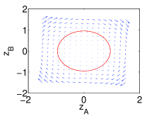
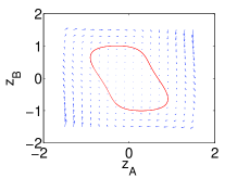
We have verified this prediction also numerically. First, panels (g), (h), and (i) of Fig. 1 show direct simulations of the four-state model with increasing values of the asymmetry parameter $r$. One sees that the visual appearance of the patterns is modified due to the phase-dependent prefactor $h(\theta)$ but that the effective wave length appears to undergo no changes. Furthermore, we have systematically varied the diffusion constant $D$ for different values of $r$ studying the extinction probability. The results are shown in Fig. (2). The evident conclusion is that for small $\epsilon$ the cross-over remains untouched. Finally, we have visualized the perturbation to the limit cycles of the non-spatial dynamical system in Fig. (4).

Figure 4: (Color online) The phase-space flow and limit cycle trajectories for the non-spatial rate-asymmetric four-state model with $r=1.0$ (on the left) and $r=1.06$ (on the right). The parameters are $\mu=\sigma=1$.

IV Discussion

In this work, we have addressed two questions related to variants of the rock-paper-scissors game in which the total density is not conserved. First, we have shown that the spiral formation observed in the four-state case is a property of the four-state case only, and does not generalize to the more widely studied three-state rock-paper-scissors game with conserved total density. The spiral formation has been previously argued reichenbach2007 to lead to a cross-over from coexistence of all three populations to an absorbing state with one surviving population and the other two extinct. The mechanism has been considered to be explicitly spiral-formation induced since the cross-over takes place at exactly that value of the parameters where the spiral wave length becomes equal to the linear size of the system. Here, we have shown that a similar cross-over takes place in the three-state model as well even though there are no signs of spiral (or any other visible pattern) formation at all. We have identified that the mechanism of the said cross-over is the appearance of a length scale from the interplay between fluctuations and diffusion.

This result has direct consequences regarding the stability of such systems or, put in other words, the extent to which biodiversity is maintained. Namely, the message is that in cyclically dominating systems of three species, fast diffusion or big mobility can destroy species coexistence regardless of whether there is a conservation law of total density in the system or not. The mechanism can either show up as visible pattern formation (here, the four-state case) or not (the three-state case). However, attention has to be paid to the details of the system if quantitative predictions are to be made. The value of the diffusion constant at which the destruction of coexistence is observed can differ by more than an order of magnitude for different cases (see Fig. 2). The result also hints to the direction that the law of conservation of total density might play a role in pattern formation in more complicated cases as well (see Ref. szabo2008 , for instance).

Furthermore, the previous studies have considered only the cases where the reaction rates between all pairs of species are equal. This could potentially be a serious limitation since such equalities do not exist in reality, generally loose2008 . We have extended the previously defined four-state model reichenbach2007 to cases where the reaction rates are not equal. By looking at the first-order perturbation from the case with equal densities, we have been able to map this case to a partial differential equation that, in turn, can be turned into the complex Ginzburg-Landau equation with a transformation of variables that does not alter the qualitative properties of the system in the first order. In particular, the effective wave length of the spirals equals that of the case with equal densities. As a conclusion, a small asymmetry in the reaction rates does not change either the properties of the pattern formation nor the location of the cross-over to the absorbing state. Altogether, this result serves to give a partial explanation why pattern formation and cross-over to extinction are visible in experiments as well. The behavior at larger asymmetries remains to be explored.

References

- (1) I. S. Aranson and L. Kramer, Rev. Mod. Phys. 74, 99 (2002).
- (2) V. P. Zhdanov, Surf. Sci. Rep. 45, 231 (2002).
- (3) R.V. Solé and J. Bascompte, Self-Organization in Complex Ecosystems, Princeton University Press, Princeton (2006).
- (4) B. Kerr, M. A. Riley, M. W. Feldman, and B. J. M. Bohannan, Nature 418, 171 (2002).
- (5) T. Reichenbach, M. Mobilia, and E. Frey, Nature 448, 1046 (2007).
- (6) C. Briggs and M.F. Hoopes, Theor. Pop. Biol. 65, 299 (2004).
- (7) G. Szabo, M. A. Santos, and J. F. F. Mendes, Phys. Rev. E 60, 3776 (1999).
- (8) G. Szabo, A. Szolnoki, and R. Izsák, J. Phys. A. Math. Gen. 37, 2599 (2004).
- (9) A. Szolnoki and G. Szabo, Phys. Rev. E 70, 037102 (2004).
- (10) T. Reichenbach, M. Mobilia, and E. Frey, Phys. Rev. E 74, 051907 (2006).
- (11) J. C. Claussen and A. Traulsen, Phys. Rev. Lett. 100, 058104 (2008).
- (12) G. Szabo and A. Szolnoki, Phys. Rev. E 65, 036115 (2002).
- (13) A. Szolnoki and G. Szabo, Phys. Rev. E 70, 027101 (2004).
- (14) A. Szolnoki, G. Szabo, and M. Ravasz, Phys. Rev. E 71, 027102 (2005).
- (15) H. Nishiuchi, N. Hatano, and K. Kubo, e-print, arXiv/0801.4859.
- (16) G. Szabo, A. Szolnoki, and I. Borsos, e-print, arXiv/0801.4543.
- (17) J. Keymer, P. Galadja, C. Muldoon, S. Park, and R. H. Austin, Proc. Nat. Acad. Sci. 103, 17290 (2006).
- (18) M. Loose, E. Fischer-Friedrich, J. Ries, K. Kruse, and P. Schwille, Science 320, 789 (2008).
- (19) B. Sinervo and C. M. Lively, Nature 380, 240 (1996).
- (20) B. C. Kirkup and M. A. Riley, Nature 428, 412 (2004).
- (21) D. Semmann, H.-J. Krambeck, and M. Milinski, Nature 425, 390 (2003).
- (22) T. Reichenbach, M. Mobilia, and E. Frey, e-print, arXiv/0801.1798.
- (23) K.-i. Tainaka, Phys. Rev. Lett. 63, 2688 (1989).
- (24) K.-i. Tainaka, Phys. Rev. E 50, 3401 (1994).
- (25) J. Marro and R. Dickman, Nonequilibrium Phase Transitions in Lattice Models, Cambridge University Press, Cambridge (1999).
- (26) W. G. Dantas, M. J. de Oliveira, and J. F. Stilck, e-print, arXiv/0705.0317.
- (27) A. Messer and H. Hinrichsen, e-print, arXiv/0802.2789.
- (28) M. Peltomäki, M. Rost, and M. Alava, submitted.