Thermal memory: a storage of phononic information
Abstract
Memory is an indispensable element for computer besides logic gates. In this Letter we report a model of thermal memory. We demonstrate via numerical simulation that thermal (phononic) information stored in the memory can be retained for a long time without being lost and more importantly can be read out without being destroyed. The possibility of experimental realization is also discussed.
pacs:
85.90.+h 07.20.Pe 63.22.-m 89.20.FfUnsatiable demands for thermal management/control in our daily life ranges from thermal isolating to efficient heat dissipation have driven us to better understand heat conduction from molecular level. Recent years has witnessed a fast development including theoretical proposals in functional thermal devices such as thermal diode that rectifies heat current diode , thermal transistor that switches and modulates heat current transistor , heat pump that carries heat against temperature bias heatpump , and experimental works such as nanotube phonon waveguide waveguide , thermal conductance tuning thermaltuning and nano-scale solid state thermal rectifier experimentaldiode . More importantly, logic operations with phonons/heat have been demonstrated theoreticallythermalgate , which, in principle, has opened the door for a brand new subject - phononics - a science and engineering of processing information with heatphononics . The question arises naturally and immediately: whether a thermal (phononic) memory that can store information is possible?
In this Letter, we would like to give a definite answer by studying the transient process, which in fact exhibits much richer phenomena than asymptotical stationary state does, of a non-equilibrium system. This topic has been however rarely studied so far.
Like an electronic memory that records data by maintaining voltage in a capacitance, a thermal memory stores data by keeping temperature somewhere. An ideal memory keeps the data forever without fading. This is never possible for a thermal system because sooner or later randomness of the heat (fluctuation) will eliminate any record of the history. However this problem is not serious from application point of view since we only need to maintain the data until we refresh it or read it. This is exactly the case for the widely used Dynamic Random Access Memory (DRAM) that needs refresh operation regularly. Any system that keeps temperature (thus data) somewhere for a very long time might be a candidate for thermal memory, such as breather and localized harmonic mode etc. However perturbation is unavoidable in a thermal system, especially as the data are read (i.e., the local temperature is measured). The breather and harmonic mode, even if do not collapse immediately under the perturbationbreather , are not able to recover their original state. Because the energy that is changed by the perturbation, e.g., the necessary energy exchange in order to build equilibrium between the system and the thermometer during the data reading (temperature measuring) process, is not recoverable in the autonomous systems without an external energy source/sink. We thus have to turn to a thermal-circuit with power supply, i.e., driven by external heat bath.
Like an electric circuit, the temperature and heat current distributions of a thermal-circuit are determined by Kirchhoff’s laws. In any linear thermal-circuit, i.e. all thermal resistances are fixed, independent of temperature and/or temperature drop, the steady state that satisfies Kirchhoff’s laws must be unique. This unique state must be stable, namely under any perturbation the system will eventually return to this state. However in order to work as a thermal memory, a thermal-circuit must have more than one stable steady states, such a bi-stable thermal-circuit is only possible in the presence of nonlinear thermal devices.
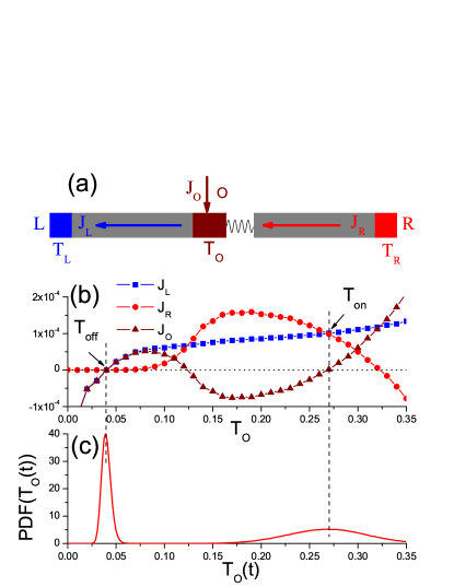
To make such a thermal-circuit, we consider a one dimensional nonlinear lattice that consists of two Frenkel-Kontorova (FK) segments FK sandwich a central particle in between. Its configuration is shown in Fig.1(a) and its Hamiltonian follows:
| (1) |
and the Hamiltonian of each segment can be written as =, with denotes the displacement from equilibrium position of the particle in segment . We have set the mass of each particle to unity. The parameters and are the harmonic spring constant and the on-site potential of the FK segments. We couple the last particles of segments and to particle via harmonic springs. Thus =. In our numerical simulation, segment and each contains 50 particles. Fixed boundary conditions are applied. Other parameters are: ==0.45, =0.2, =0.05, =10, =0, =10. The deep valley of on-site potential of particle , , and the weak coupling between segment and particle , , induce a negative differential thermal resistance (NDTR)transistor between and segment , which is the key for the model of thermal memory. We use a wavy curve to stress this in Fig.1(a). and , temperatures of the power supplies (heat baths) that contacted to the ends of the two segments, are fixed to and , respectively. Without these energy resource/sink, the system reduces to an autonomous one thus, as has been explained above, is not able to work as a thermal memory. All heat baths are simulated by Langevin heat baths review .
Because of NDTR, with fixed and a control heat bath with adjustable temperature is coupled to the particle , there exist more than one values of with which the heat current from control heat bath to particle , , is zerotransistor , as shown in Fig.1(b). Suppose the temperature of is initially set to either “” or “” by the control heat bath. After the control heat bath is removed the state will remain unchanged for a long time, in spite of the thermal fluctuation. Because as the consequence of the small perturbation which slightly changes the temperature , the changes of heat currents and always pull back, thus these two states are “stable”. It is easy to check the other steady state in between is however unstable.
In the equilibrium state of an Hamiltonian system with ergodicity, temperature can be defined as twice of the average kinetic energy per degree of freedom. In order to study transient process, the “finite time temperature” is naturally defined as, for a 1D system, twice of the average kinetic energy in a time window , i.e.,: Hereafter, any temperature which is a function of time means the finite time temperature. Due to the thermal fluctuation, even in a steady state, finite time temperature has different value at different time window. The probability density function (PDF) of the finite time temperature is thus defined accordingly. If the time window is chosen to be too long, the PDF approaches a function locates at “infinite time” temperature , while if is too short, big thermal fluctuation dominates thus the distribution is more or less a Maxwell energy distribution. In the medial cases PDF presents much more information other than the value of temperature itself. In this Letter, is fixed to dimensionless time units. Since the frequency of the system we studied is about 0.2 transistor , this period of time covers about 2,000 oscillations, thus is a microscopical long time.
Since “on” and “off” are two stable states, the finite time temperature of the particle in the absence of control heat bath is expected to stay around and with much higher probability than elsewhere. In Fig.1(c) the locations of the two peaks clearly confirms this expectation. By adjusting parameters of the system, the values of and and the peaks shift simultaneously but always coincide with each other.
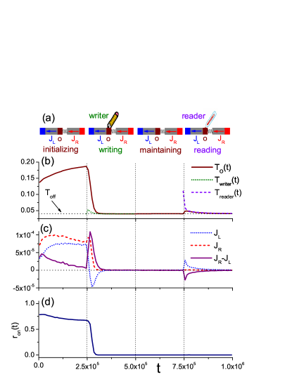
We have so far confirmed the stability of the two states “on” and “off” of the model. In the following, we shall demonstrate a complete, four-stage, writing-reading process of the thermal memory, as is shown in Fig.2(a). During the whole process the left and right ends of the memory are always connected to two power supply heat baths with temperatures and , respectively. Stage 1: initializing the memory. Each particle is initially set a velocity chosen from a Gaussian distribution corresponding to a temperature in . After some time the system approaches to an asymptotic state, thus saturates, see Fig.2(b). Stage 2: writing the datum into the memory. In our simulation, the “writer” is simulated by a FK lattice with =10 particles and identical parameters with segment . It is connected via a linear spring with =1.0, at its one end, to the particle of the memory. The temperature of the writer is initially set to and the other end is connected to a heat bath with temperature also. In a short time the writer cools down to , namely the datum “off” has been written into the memory. Stage 3: maintaining the datum in the memory. In this stage, the writer is removed from the memory. And we can see from Fig.2(b) that remains nearly unchanged during this stage, which means that the datum stored in the memory can last for a long time. Stage 4: reading out the datum from memory. A “reader”(thermometer) is used to read the datum out from the memory. Here the “reader” is simulated by the same FK lattice as the writer. It is connected, to the particle of the memory. The temperature of the reader is initially set to a middle temperature between and (in this Letter it is 0.11). Different from the writer, the reader is not connected to any heat bath. This stage is the most important and most interesting one. We see that at the beginning the particle is temporarily warmed up because the reader is hotter. However, since the “off” state is stable, and also the temperature of the reader are cooled down to shortly, implying that the datum has been successfully read out. To gain a clearer picture, we show the heat currents through the two segments and in the Fig.2(c). At the beginning of the reading stage since the temperature of particle is warmed up by the reader, as a response of the increase of , increases a lot whereas increases only very little, thus the net current - changes from zero to negative, i.e., the power supply (left end heat bath) absorbs heat from the particle . This is the reason that can be cooled down and recovered to automatically.
The results shown in Fig.2 are obtained from an ensemble average over independent samples. For a model of thermal memory, the ratio of samples that keep the correct data is an important feature. To describe this quantitatively, we calculate the ratio of “on” state: , while is the total number of samples stay at “on” state at time and is the total number of samples. We define, at time , a sample is at “on” state if the finite time temperature of its particle is greater than a critical value =0.11. we show during the whole process in Fig.2(d). It is clearly seen that after the writing stage, always keeps at a very low level, even under the not-very-small perturbation from the hot reader. The discrepancy between and 0 is in the order of , which means two or three “errors” among the 20,000 samples, is even indistinguishable in the figure by eye, namely the memories successfully maintain the data “off” that are initially set by the writer, the data are hardly destroyed even after being read!
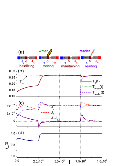
It has been pointed out that, to be a memory, the system must have more than one stable steady states around which the above writing-reading process can be completed, thus in the following we demonstrate the writing-reading process around the other stable steady state, the “on” state in Fig.3. The difference from Fig.2 is that in the second stage the writer is set to temperature and connected to a heat bath with temperature . We see in this stage changes to shortly. In the consequent maintaining stage keeps unchanged at . In the reading stage: the reader is initially set to the same temperature as before. We see at the beginning because this time the reader is colder, the particle is temporarily cooled down, as a response decreases while increases, thus the net current - becomes positive, which warms up the particle (also the reader) and recovers its temperature to . The datum “on” is again read out successfully. As for , see Fig.3(d). This time keeps at a very high level. The discrepancy between and 1 is again at the order of , namely the datum “on” can be successfully maintained in and read out from memory.
Finally we would like to discuss the lifetime of data in the thermal memory. In an electric DRAM, since real capacitors leak charge, the data will eventually fade unless the capacitor charge is refreshed periodically (about ). Similarly, we find a few “errors” among the many samples that we studied at the end of the writing-reading process. Suppose the data fading process is a Poisson process then the average lifetime of the data is roughly dimensionless time units which contains about periods of oscillation. This corresponds to 100 if the memory is made of carbon nanostructures such as nanotubecarbon , in which the key of the model, NDTR has been found numericallyWuLi0708 . This lifetime is unsatisfying when compared with an electronic DRAM. However this value can be easily and greatly enlarged by parallel combining more identical memories together. The dynamics of finite time temperature of particle , around either of the two stable steady states can be roughly described by an autoregressive diffusion process, say, the simplest one, Ornstein-Uhlenbeck (OU) process: . Where corresponds to relative to or . represents the effect of the response net heat current that pulls back to zero and is a Gaussian white noise with zero mean and fixed variance which describes fluctuation of the heat current. The mean first passage time (MFPT) through a certain boundary (which denotes or ) conditional upon represents the average lifetime of the data in the memory. In the limiting case that , MFPT, where MFPT_OU . MFPT diverges rapidly as decreases. Parallel combining identical memories together decreases by times while keeps unchanged, thus increases the average lifetime of data greatly. Such a fast divergence tendency of MFPT has also been widely found in a class of diffusion processes with steady state distribution OUexample , thus the above conclusion is not limited to the specified process, the OU process.
In summary, we have demonstrated the feasibility of thermal memory from a bistable thermal-circuit. The information stored in such a thermal memory can last very long time and, more importantly it is self-recoverable under the not-very-small perturbation from the thermometer when the data are read. With the rapid developing nano-technology waveguide ; thermaltuning ; experimentaldiode , the thermal memory should be realized in nanoscale systems experimentally in a foreseeable future.
The work is supported in part by the start-up grant of Renmin University of China (LW) and Grant R-144-000-203-112 from Ministry of Education of Republic of Singapore, and Grant R-144-000-222-646 from NUS.
References
- (1) M. Terraneo, M. Peyrard, and G. Casati, Phys. Rev. Lett. 88, 094302 (2002); B. Li, L. Wang, and G. Casati, Phys. Rev. Lett. 93, 184301 (2004); D. Segal and A. Nitzan, Phys. Rev. Lett. 94, 034301 (2005); B. Li, J. Lan and L. Wang, Phys. Rev. Lett. 95, 104302 (2005); B. Hu, L. Yang, and Y. Zhang, Phys. Rev. Lett. 97, 124302 (2006); D. Segal, Phys. Rev. Lett. 100, 105901 (2008).
- (2) B. Li, L. Wang, and G. Casati, Appl. Phys. Lett 88, 143501 (2006); D. Segal, Phys. Rev. E 77 021103 (2008); W. Lo, L. Wang, and B. Li, J. Phys. Soc. Jpn., 77, 054402 (2008).
- (3) D. Segal and A. Nitzan, Phys. Rev. E 73, 026109 (2006); R. Marathe, A. M. Jayannavar, and A. Dhar, Phys. Rev. E 75, 030103 (2007).
- (4) C. W. Chang et al, Phys. Rev. Lett. 99, 045901 (2007).
- (5) C. W. Chang et al, Appl. Phys. Lett 90, 193114 (2007).
- (6) C. W. Chang et al, SCIENCE, 314, 1121 (2006).
- (7) L. Wang and B. Li, Phys. Rev. Lett. 99, 177208 (2007).
- (8) L. Wang and B. Li, Phys. World 21, no.3, 27 (2008).
- (9) S. Flach and A. Gorbach, Physics Reports (2008), doi:10.1016/j.physrep.2008.05.002
- (10) O. M. Braun and Y. S. Kivshar, Phys. Rep. 306, 1 (1998); B. Hu, B. Li, and H. Zhao, Phys. Rev. E 57, 2992 (1998).
- (11) F. Bonetto et al., in Mathematical Physics 2000, edited by A. Fokas et al.. (Imperial College Press, London)2000, pp. 128-150.
- (12) The oscillation frequency of atoms in carbon nanotube is about 10THz, see, for example S. Rols et al, Phys. Rev. Lett. 85, 5222 (2000).
- (13) G. Wu and B. Li, Phys. Rev. B 76, 085424 (2007); J. Phys.: Condens. Matter 20, 175211 (2008).
- (14) A. G. Nobile, L. M. Ricciardi and L. Sacerdote, J. Appl. Prob. 22, 360 (1985). L. M. Ricciardi and S. Sato, J. Appl. Prob. 25, 43 (1988).
- (15) A. G. Nobile, L. M. Ricciardi, and L. Sacerdote, J. Appl. Prob. 22, 611 (1985).