The evolution of anisotropic structures and turbulence in the multi-dimensional Burgers equation

Abstract

The goal of the present paper is the investigation of the evolution of anisotropic regular structures and turbulence at large Reynolds number in the multi-dimensional Burgers equation. We show that we have local isotropization of the velocity and potential fields at small scale inside cellular zones. For periodic waves, we have simple decay inside of a frozen structure. The global structure at large times is determined by the initial correlations, and for short range correlated field, we have isotropization of turbulence. The other limit we consider is the final behavior of the field, when the processes of nonlinear and harmonic interactions are frozen, and the evolution of the field is determined only by the linear dissipation.

I Introduction

The well known Burgers equation describes a variety of nonlinear wave phenomena arising in the theory of wave propagation, acoustics, plasma physics and so on (see, e.g., Whitham ; RudenkoSoluyan ; GMS91 ; WW98 ; FB2001 ; BKh2007 ). This equation was originally introduced by J.M.Burgers as a model of hydrodynamical turbulence Burgers1939 ; Burgers1974 . It shares a number of properties with the Navier–Stokes equation : the same type of nonlinearity, of invariance groups and of energy-dissipation relation, the existence of a multidimensional version, etc Frisch . However, Burgers equation is known to be integrable and therefore lacks the property of sensitive dependence on the initial conditions. Nevertheless, the differences between the Burgers and Navier-Stokes equations are as interesting as the similarities Kr68 and this is also true for the multi-dimensional Burgers equation :

$$\frac{\partial{\bf v}}{\partial t}+\left({\bf v}\cdot\nabla\right){\bf v}=\nu\nabla^{2}{\bf v}\,,$$ (1)

With external random forces the multi-dimensional Burgers equation is widely used as a model of randomly driven Navier-Stokes equation without pressure CheklovYakhot ; Polyakov ; EKMS ; Boldyrev99 ; DMTRS01 . The three–dimensional form of equation has been used to model the formation of the large scale structure of the Universe when pressure is negligible. Known as ”adhesion” approximation this equation describes the nonlinear stage of gravitational instability arising from random initial perturbation GurbatovSaichev1984 ; GSS89 ; SZ89 ; VDFN94 ; ASG2008 . Other problems leading to the multi–dimensional Burgers equation, or variants of it, include surface growth under sputter deposition and flame front motion BS95 ; KM96 . In such instances, the potential ${\psi}$ corresponds to the shape of the front’s surface, and the equation for the velocity potential ${\psi}$ is identical to the KPZ (Kardar, Parisi, Zhang) equation BS95 ; KardarParisiZhang ; WW98 ; BMP95 . For the deposition problem the velocity in multi–dimensional Burgers equation ${\bf v}=-\nabla\psi$ is the gradient of the surface. The mean–square gradient $E(t)=\langle(\nabla{\psi}({\bf x},t))^{2}\rangle=\langle{\bf v}^{2}({\bf x},t)\rangle$ is a measure of the roughness of the surface and may either decrease or increase with time.

When the initial potential $\psi_{0}({\bf x})$ is a superposition of one dimensional potentials $\psi_{0,i}(x_{i})$, namely $\psi_{0}({\bf x})=\sum_{i}\psi_{0,i}(x_{i})$ and $v_{0,i}({\bf x})=v_{0,i}(x_{i})$, there are no interaction between the velocity component $v_{0,i}({\bf x},t)=v_{0,i}(x_{i},t)$ and evolution of each component is determined by one-dimensional Burgers equation. Before the description evolution of fields in multi-dimensional Burgers equation we discuss now very short the evolution of basic types of perturbation in one-dimensional Burgers equation Whitham ; RudenkoSoluyan ; GMS91 ; WW98 , and compare the behaviour of “plane” orthogonal waves in 2-dimensional Burgers equation with different initial spatial scales.

At infinite Reynolds number ($\nu\rightarrow 0$) the harmonic perturbation $v_{0}(x)=k_{0}\psi_{0}\sin{k_{0}x}$ ($\psi_{0}(x)=\psi_{0}\cos{k_{0}x}$), is transformed at $t\gg t_{\rm nl}=1/k_{0}^{2}\psi_{0}$ into saw-tooth wave with gradient $\partial v/\partial x=1/t$ and the same period $L_{0}=2\pi/k_{0}$. It’s important that at this stage the amplitude $a=L_{0}/t$ and the energy $E(t)=L_{0}^{2}/12t^{2}$ doesn’t depend on the initial amplitude. Thus if we compare the evolution of two components $v_{0,i}(x_{i},t)$ with equal potential $\psi_{0}$ and different scales $L_{i}$ $(L_{1}<<L_{2})$, the initial energy will be much higher for the component with smaller scale $E_{1}(0)/E_{2}(0)=L_{2}^{2}/L_{1}^{2}$. But asymptotically we have inverse situation $E_{1}(t)/E_{2}(t)\rightarrow{L_{1}^{2}}/{L_{2}^{2}}$. For large but finite Reynolds number ${\rm Re}_{0}=\psi_{0}/2\nu$ the shock fronts have a finite width $\sim\nu t/L_{0}$ and at $t\gg t_{\rm nl}{\rm Re}_{0}$ we have a linear stage of evolution where $v(x,t)=4\nu k_{0}\sin(k_{0}x)\exp(-\nu k_{0}^{2}t)$.

Continuous random initial fields are also transformed into sequences of regions (cells) with the same gradient $\partial v/\partial x=1/t$, but with random position of the shocks separating them. The merging of the shocks leads to an increase of the integral scale of turbulence $L(t)$ and because of this the energy $E(t)\sim L^{2}(t)/t^{2}$ of random field decreases more slowly than the energy of periodic signal. The type of the turbulence evolution is determined by the behaviour of large scale part of the initial energy spectrum $E_{0}(k)\sim\alpha^{2}k^{n}$. For $n<1$ the initial potential is Brownian or fractional Brownian motion and scaling argument may be used Burgers1974 ; GMS91 ; WW98 ; VDFN94 ; SheAurellFrisch ; FrMart99 . In this case the turbulence in self-similar and with integral scale $L(t)=(\alpha t)^{\frac{2}{3+n}}$. For $n>1$ the law of energy decay strongly depends on the statistical properties of the initial field WW98 ; AMS94 ; EsipovNewman ; Esipov ; Newman97 ; Gurbatov2000 .

For an initial Gaussian perturbation the integral scale $L(t)$ and the energy of the turbulence $E(t)$

$$L(t) = (t\sigma_{\psi})^{1/2}\ln^{-1/4}\left(\frac{t\sigma_{\psi}}{2\pi l_{0}^{2}}\right)\ ,$$

$$E(t) = L^{2}(t)/t^{2}$$ (2)

are determined only by two integral characteristic of the initial spectrum : the variance of initial potential ${\sigma_{\psi}}^{2}=\langle\psi_{0}^{2}\rangle$ and the velocity $\sigma_{v}^{2}=\langle v_{0}^{2}\rangle$ Burgers1974 ; GMS91 ; Kida ; GurbatovSaichev1981 ; FournierFrisch ; MSW95 ; GSAFT97 ; NGAS2005 . Here $l_{0}=\sigma_{\psi}/{\sigma_{v}}$ is the integral scale of initial perturbation, and $\sigma_{\psi}/l_{0}^{2}=t_{\rm nl}$ is the nonlinear time. Thus the energy of two components with equal initial potential variance $\sigma_{\psi}$ and different scales $l_{0,i},(l_{0,1}\ll l_{0,2})$ will have very large difference at $t=0$; ${E_{1}(0)}/{E_{2}(0)}={l_{2}^{2}}/{l_{1}^{2}}\gg 1$ and with logarithmic correction will be the same at large time ${E_{1}(t)}/{E_{2}(t)}\simeq 1$. For large, but finite Reynolds number ${\rm Re}_{0}=\sigma_{\psi}/2\nu$ the shock fronts have a finite width $\sim\nu t/L(t)$ and due to the multiple merging of shocks the linear regime take place at very large times $t\gg t_{\rm nl}\exp({\rm Re}_{0}^{2})/{\rm Re}_{0}$. At linear stage the energy decays as $Ct^{-3/2}$, where $C\sim L_{0}\exp({\rm Re}_{0}^{2})/{\rm Re}_{0}$.

The goal of the present paper is the investigation of the evolution of anisotropic regular structures and turbulence at large Reynolds number, when we have a multiple interaction of the spatial harmonics of the initial perturbation. We shown that we have local isotropization of the velocity and potential fields inside the cells. For the periodic wave we have the decay of frozen structure. The global structure of the random field is determined by the long correlation of initial field, and for the short correlated field we have isotropization of turbulence. The other limit we consider in the paper is the old-age behaviour of the field, when the processes of nonlinear self-action and harmonic interaction seems to be frozen, and the evolution of the field is determined only by the linear dissipation.

The paper is organized as follows. In Section II we formulate our problem and list some results about the solution of multidimensional Burgers equation in the limit of vanishing viscosity and its old age behavior. We also shown that we have local isotropization of the velocity and potential fields. In Section III we consider the interaction of plane waves and evolution of periodic structures in 2-d Burgers equation. In Section IV we consider the evolution of anisotropic multidimensional Burgers turbulence in inviscosid limit. We also discuss here the influence of finite viscosity and long range correlation on the late stage evolution of Burgers’ turbulence.

II Multi-dimensional Burgers equation, the limit of vanishing viscosity and the old age behaviour

We shall be concerned with the initial value problem for the un-forced multi-dimensional Burgers equation (1) and consider only the potential solution of this equation, namely

$$\bf v(\bf x,t)=-\nabla\psi(\bf x,t)\ .$$ (3)

The velocity potential $\psi({\bf x},t)$ satisfies the following nonlinear equation

$$\frac{\partial{\psi}}{\partial t}=\frac{1}{2}(\nabla{\psi})^{2}+\nu\nabla^{2}\psi\ .$$ (4)

The equation for the velocity potential $\psi$ is identical to the KPZ (Kardar, Parisi, Zhang) equation BS95 ; KardarParisiZhang ; WW98 , which is usually written in the terms of the variable $h=\lambda^{-1}\cdot\psi$. The parameter $\lambda$ has the dimension of length divided by time and is the local velocity of the surface growth. Henceforth $h(\bf x,t)$ has the dimension of length and is the measure of the surface’s shapeness. In this case ${\bf v}=-\nabla\psi$ is the gradient of the surface. The roughness of the surface is measured by its mean-square gradient

$$E(t)=\langle(\nabla{\psi}({\bf x},t))^{2}\rangle=\langle{\bf v}^{2}({\bf x},t)\rangle=\sum_{i}E_{i}(t)\ ,$$ (5)

Here the angular brackets denote ensemble averages or space averages for periodic structures. For the one-dimensional homogeneous field $E(t)$ is the density of energy and always decreases with time. At the initial stage of evolution and in the limit of vanishing viscosity the multi-dimensional Burgers equation is equal to the free motion of the particles. In Lagrangian representation the velocity of the particle ${\bf V}(t;{\bf y})$ is a constant. Here ${\bf y}$ is initial (Lagrangian) coordinate of the particle. In one-dimensional case the increasing of the length of elementary Eulerian interval $\Delta x=\Delta y+t\Delta V$ is compensated by the decreasing of length $\Delta x=\Delta y-t\Delta V$ of the steepening interval and therefore the energy of the wave (the mean roughness of the curve) is conserved. After shock formation(s), the energy of the wave decreases with time. In multi-dimensional case the changing of elementary Eulerian volume depends also on the initial curvature of perturbation and we don’t generally have compensation of steepening and stretching volumes. Thus for $d>1$ the roughness of the surface, measured by its mean-square gradient $E(t)$ (see (5)) may either decrease or increase with time AMS94 ; Gurbatov2000 . The increase of the mean-square gradient in the multi-dimensional Burgers equation (in contrast with $d=1$) is the result of this equation not having a conservation form. Nevertheless we will use the expression ”turbulence energy” for the value of $E(t)$ and call $E_{i}(t)=\langle(\partial{\psi}/\partial{x_{i}})^{2}\rangle=\langle v_{i}^{2}\rangle$ the energy of the $i$-th velocity component.

Using the Hopf-Cole transformation Hopf ; Cole

$$\psi({\bf x},t)=2\nu\log U({\bf x},t)\ ,$$ (6)

one can reduce equation (1) to the linear diffusion equation

$$\frac{\partial{U}}{\partial t}=\nu\nabla^{2}U\,,\;\;\ U({\bf x},0)=U_{0}({\bf x})=\exp\left[\frac{\psi_{0}({\bf x})}{2\nu}\right]\ .$$ (7)

The goal of the present paper is the investigation of the evolution of regular structures and turbulence at large Reynolds number. For the not very large times we can use the the solutions of Burgers equation in the limit of vanishing viscosity. The other limit is the old-age behaviour of the field, when the processes of nonlinear self-action and harmonic interaction seems to be frozen, end the evolution of the field is determined only by the linear dissipation. In this case we have the linearisation of Hopf Cole transformation (6).

In the limit of vanishing viscosity $\nu\rightarrow 0$ use of Laplace’s method leads to the following ”maximum representation” for the potential velocity field Hopf ; GMS91 ; VDFN94  :

$$\psi({\bf x},t)=\max_{{\bf y}}\Phi({\bf x},{\bf y},t)\ ,$$ (8)

$$\Phi({\bf x},{\bf y},t)=\psi_{0}({\bf y})-\frac{({\bf x}-{\bf y})^{2}}{2t}\ ,$$ (9)

$${\bf v}({\bf x},t)=\frac{{\bf x}-{\bf y}({\bf x},t)}{t}={\bf v}_{0}({\bf y}({\bf x},t))\ .$$ (10)

Here $\psi_{0}({\bf y})$ is the initial potential and ${\bf v}_{0}({\bf x})=-\nabla\psi_{0}({\bf x})$. In (10) ${\bf y}({\bf x},t)$ is the Lagrangian coordinate where the function $\Phi({\bf x},{\bf y},t)$ achieves its global or absolute maximum for a given coordinate ${\bf x}$ and time $t$. It is easy to see that ${\bf y}$ is the Lagrangian coordinate from which starts the fluid particle which will be at at the point ${\bf x}$ the moment $t$ GMS91 .

At large times the paraboloid peak in (9) defines a much smoother function than the initial potential $\psi_{0}({\bf y})$. Consequently, the absolute maximum of $\Phi({\bf x},{\bf y},t)$ coincides with one of the local maxima of $\psi_{0}({\bf y})$. In the neighborhood of local maximum $\bf{y_{k}}$ we can represent the initial potential in the following form

$$\psi_{0}({\bf x})=\psi_{0,k}\left(1-\sum_{i}\frac{(x_{i}-y_{i,k})^{2}}{2L_{i}^{2}}\right)\ ,$$ (11)

where $x_{i}$ now are the principle axis of the local quadratic form describing the potential near the local maximum. At relatively large time the Eulerian velocity field ${\bf v}({\bf x},t)$ in the whole space will be determined by the particles moving away from the small regions near the local maximum of $\psi_{0}(\bf x)$ :

$${y_{i}}({\bf x},t)=\frac{(x_{i}-y_{i,k})}{(1+\psi_{0,k}t/L_{i}^{2})}\ .$$ (12)

Then, the Lagrangian coordinate ${\bf y}({\bf x},t)$ becomes a discontinuous function of ${\bf x}$, constant within a cell, but jumping at the boundaries GMS91 ; VDFN94 . The velocity field ${\bf v}({\bf x},t)$ has discontinuities (shocks) and the potential field $\psi({\bf x},t)$ has gradient discontinuities (cusps) at the cell boundaries. From (10),(12) it becomes clear that inside the cells the velocity and potential fields have a universal isotropic and self-similar structure :

$$\psi({\bf x},t)=\psi_{0}({\bf y}_{k})-\frac{({\bf x}-{\bf y}_{k})^{2}}{2t}\ .$$ (13)

$${\bf v}({\bf x},t)=\frac{{\bf x}-{\bf y}_{k}}{t}\ .$$ (14)

One can see that due to the nonlinearity there’s the local isotropisation of the velocity field in the neighborhood of the local maximum of $\psi_{0}(\bf x)$. The longitudinal component of the velocity vector ${\bf v}({\bf x},t)$ consists of a sequence of sawtooth pulses, just as in one dimension. The transverse components consist of sequences of rectangular pulses. At large times the global structure and evolution of the velocity and potential fields will be determined by the properties of local maxima $\psi_{0}({\bf y}_{k})$. For the random field wall motion results in continuous change of cell shape with cells swallowing their neighbors and thereby inducing growth of the external scale $L(t)$ of the Burgers turbulence.

Let us now discuss the old-age limit of the solution of Burgers equation. Consider a group of perturbation with the bounded initial potential $\langle\psi_{0}({\bf x})^{2}\rangle<\infty$ assuming that $\psi_{0}({\bf x})$ is a periodic structure or homogeneous noise with rather fast decreasing probability distribution of the potential $\psi_{0}$. For such a perturbation in $U({\bf x},t)$ we separate a constant component $\bar{U}$ :

$$U({\bf x},t)=\bar{U}+\tilde{U}({\bf x},t)=\bar{U}\left(1+u({\bf x},t)\right)\;\;.$$ (15)

Here $u({\bf x},t)=\tilde{U}({\bf x},t)/\bar{U}$ is the relative perturbation of field $U({\bf x},t)$. Inserting (15) into (7) we see that $\bar{U}$ does not depend on time. Here $\tilde{U}_{0}({\bf x})$ and $u_{0}({\bf x})$ are fields with zero mean value (on the period or statistically for noise). As times goes on, the viscous dissipation and oscillation (inhomogeneity) smoothing causes the amplitude (variance) of the field $\tilde{U}({\bf x},t)$ to become less. At times when its relative amounts $\tilde{U}$ is small in compare with $\bar{U}$ ($|u|\ll 1$) the solution (6) is equal to

$${\bf v}({\bf x},t)=-2\nu\nabla\tilde{U}({\bf x},t)/\bar{U}=-2\nu\nabla u({\bf x},t)\;\;.$$ (16)

As $\tilde{U}({\bf x},t)$ and $u({\bf x},t)$ satisfy the linear diffusion equation, then ${\bf v}({\bf x},t)$ also at these times fulfills the linear equation. This testifies precisely to the fact that the evolution of the velocity field enters the linear stage. The accumulated nonlinear effects are described in this solution by the nonlinear integral relation between the initial velocity field ${\bf v}_{0}({\bf x})$ and the fields $\tilde{U}({\bf x},0)$, $\bar{U}$ (3,7), and are characterized by the value $|\Delta\psi_{0}|/\nu\sim{\rm Re}_{0}$. Here $\Delta\psi_{0}$ is the characteristic change in amplitude of $\psi_{0}$, and ${\rm Re}_{0}$ is the initial Reynolds number.

From (16) it is easy to get the well known result, that for ${\rm Re}_{0}\gg 1$ the initial harmonic waves asymptotically has also harmonics form, but with the amplitude not depending on the initial amplitude Whitham ; RudenkoSoluyan . At large initial Reynolds number the homogeneous Gaussian field $v_{0}(x)$ at the nonlinear stage transforms into series of sawtooth waves with strong non-Gaussian statistical properties GMS91 ; MSW95 . Nevertheless at very large time, when the relation (16) is valid, the distribution of the random field ${\bf v}({\bf x},t)$ with statistically homogeneous initial potential $\psi_{0}({\bf x})$ converges weakly to the distribution of the homogeneous Gaussian random field with zero mean value AMS94 . This stage of evolution is known as the Gaussian scenario in Burgers turbulence. In the absence of the long correlation of initial potential field the potential (and velocity consequently) have an universal covariance function GMS91 ; AMS94 . But the amplitude of this function is nonlinearly related to the initial covariance function of the field $\psi_{0}(\bf x)$ and increases proportionally $\exp(Re^{2}_{0})$ with increasing of initial Reynolds number ${\rm Re}_{0}$. When the initial potential has a long correlation ( $\langle(\psi_{0}({\bf x})\psi_{0}(0)\rangle=|{\bf x}|^{-\alpha}F({\bf x}/x)$ $,0<\alpha<3$ ) at large $x$ we have conservation at linear stage as long correlation as the anisotropy of the field $F({\bf x}/x)$ AMS94 .

III The evolution of periodic structures and the interaction of plane waves in 2-d Burgers equation

It was shown in previous section that at large time we have a cellular structure of the field with universal behaviour of potential and velocity inside each cell. The global structure of the field will be determined by the properties of local maximum of initial potential.

Let us consider the evolution of periodic structure in 2-dimensional Burgers equation

$$\psi_{0}(x_{1},x_{2})=2\psi_{0}\cos(k_{2}x_{2})\cos(k_{1}x_{1}).$$ (17)

The evolution of this structure my be interpreted as the interaction of two plane waves with equal modulus of the wave number $k_{0}$

$$\psi_{0}(x_{1},x_{2})=\psi_{0}\cos(k_{1}x_{1}+k_{2}x_{2})+\psi_{0}\cos(k_{1}x_{1}-k_{2}x_{2}).$$ (18)

Here $k_{1}=k_{0}n_{1}=2\pi/l_{1}$, $k_{2}=k_{0}n_{2}=2\pi/l_{2}$ and $\bf n$ is unit vector with the component $n_{1},n_{2}$. For the each of noninteracting plane waves the energy of $i$-th component is $E_{i,p}(t)=E(t)n_{i}^{2}$, where $E(t)$ is the energy of plane wave and $E(0)=\psi_{0}^{2}k_{0}^{2}/2$. For $\nu\rightarrow 0$ the plane wave is transformed at $t\gg t_{\rm nl}=1/k_{0}^{2}\psi_{0}$ into saw-tooth wave with gradient $\partial v/\partial x=1/t$ and the energy $E(t)=\pi^{2}/3k_{0}^{2}t^{2}$. For large but finite Reynolds number we have a linear stage of evolution where $v(x,t)=4\nu k_{0}\sin(k_{0}x)\exp(-\nu k_{0}^{2}t)$.

Consider first the late stage of evolution of periodic structure of times $t\gg t_{\rm nl}$. At this stage the velocity has the universal form in each cell (14), where ${\bf y_{k}}$ are the maximums of the initial potential (17). For the initial potential there are two sets of maximum of equal value corresponding the conditions $\cos{k_{1}x_{1}}=\cos{k_{2}x_{2}}=1$ and $\cos{k_{1}x_{1}}=\cos{k_{2}x_{2}}=-1$. The shock lines (cell boundaries) of the velocity field are orthogonal to vector connecting the neighbor cell center and they are immobile and situated in the middle between the centers. Due to the symmetry of initial conditions the velocity field is symmetric over the point $(l_{1}/2,l_{2}/2)$. Assume now that $l_{1}\leq l_{2}$ and consider the velocity fields inside the region $S$ : $\left(x_{1}\in[0,l_{1}/2],x_{2}\in[0,l_{2}/2]\right)$, see figure LABEL:fig1.

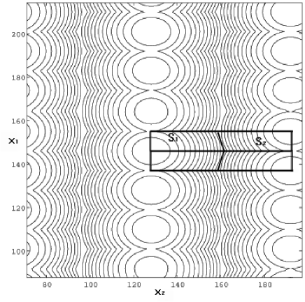
Figure 1: Cellular structure of potential for $k_{1}\gg k_{2}$.

The region $S$ is divided by the shock line in the regions $S_{1}$ and $S_{2}$

$$S_{1}:\left(0\leq x_{2}\leq-\frac{l_{1}}{l_{2}}x_{1}+\frac{l_{1}^{2}+l_{2}^{2}}{4l_{2}^{2}}\right)\;\;.$$ (19)

The center of the cell inside the region $S_{1}$ is in the point $(x_{1}=0,x_{2}=0)$ and inside the region $S_{2}$ is in the point $(x_{1}=l_{1}/2,x_{2}=l_{2}/2)$. Consequently for the velocity fields one can get

$$v_{1}=x_{1}/t,\;\;\ v_{2}=x_{2}/t,\;\;\;\;{\bf x}\in S_{1},\;\;$$

$$v_{1}=(x_{1}-l_{1}/2)/t,\;\;\ v_{2}=(x_{2}-l_{2}/2)/t,\;\;\;{\bf x}\in S_{2}.$$ (20)

Thus on large time we have a frozen structure of the field with decreasing amplitude $\sim t^{-1}$. For the energy of the velocity component from expressions (20) one can obtain

$$E_{1}(t)=\frac{l_{1}^{2}}{12t^{2}}\left(1-\frac{l_{1}^{2}}{l_{2}^{2}}\right)=\frac{\pi^{2}}{3k_{0}^{2}n_{1}^{2}t^{2}}\left(1-\frac{n_{2}^{2}}{n_{1}^{2}}\right),$$

$$E_{2}(t)=\frac{l_{2}^{2}}{48t^{2}}\left(1+\frac{l_{1}^{4}}{l_{2}^{4}}\right)=\frac{\pi^{2}}{12k_{0}^{2}n_{2}^{2}t^{2}}\left(1+\frac{n_{2}^{4}}{n_{2}^{1}}\right).$$ (21)

From (19),(20) one can receive that for the very anisotropic fields $(l_{1}\ll l_{2}),(n_{1}\simeq 1,n_{2}\ll 1)$ the velocity component $v_{1}$ reproduce the behaviour of the velocity in one-dimensional Burgers equation, but the large scale component has now the period $L=l_{2}/2$ instead of $L=l_{2}$ for the initial perturbation. Let us compare the decay of the periodic structure (17), which is a superposition of two plane waves with the decay of the energy component $E_{i,p}$ of singular plane wave. For $l_{1}\ll l_{2}$ the energy of small scale decays as $E_{1}\simeq\pi^{2}/3k_{0}^{2}n_{1}^{2}t^{2}\simeq E_{i,1}=\pi^{2}n_{1}^{2}/3k_{0}^{2}t^{2}$. The energy of large scale component $E_{2}\simeq\pi^{2}/12k_{0}^{2}n_{2}^{2}t^{2}\gg E_{i,2}=\pi^{2}n_{2}^{2}/3k_{0}^{2}t^{2}$.

Consider now the linear stage of the evolution of the periodic structure, when the Hopf-Cole solution is reduced to the linear relation (16) between the velocity field ${\bf v({\bf x},t)}$ and the solution $\tilde{U}({\bf x},t)$, $u({\bf x},t)$ of the linear diffusion equation (7). Using the relation $\exp{(z\cos{\theta})}=I_{0}(z)+2\sum_{m=1}^{\infty}I_{m}(z)\cos{m\theta}$, where $I_{m}(z)$ are a modified Bessel functions, for the solution of this equation we have from (7),(17)

$$U({\bf x},t)= \displaystyle I_{0}^{2}({\rm Re}_{0})\hfill$$ (22)

$$\displaystyle+2\sum_{m=1}^{\infty} I_{0}({\rm Re}_{0})I_{m}({\rm Re}_{0})\hfill$$

$$\{\cos[m(k_{1}x_{1}+k_{2}x_{2})]$$

$$+\cos[m(k_{1}x_{1}-k_{2}x_{2})]\}$$

$${\rm e}^{-\nu m^{2}(k_{1}^{2}+k_{2}^{2})t}$$

$$\displaystyle+2\sum_{n=1}^{\infty}\sum_{m=1}^{\infty} I_{m}({\rm Re}_{0})I_{n}({\rm Re}_{0})\hfill$$

$$\{\cos[(n+m)k_{1}x_{1}+(n-m)k_{2}x_{2}]$$

$${\rm e}^{-\nu((n+m)^{2}k_{1}^{2}+(n-m)^{2}k_{2}^{2}))t}$$

$$+\cos[(n-m)k_{1}x_{1}+(n+m)k_{2}x_{2})]$$

$${\rm e}^{-\nu((n-m)^{2}k_{1}^{2}+(n+m)^{2}k_{2}^{2})t}\}\ ,$$

where ${\rm Re}_{0}=\psi_{0}/2\nu$. Here the first sum described the nonlinear evolution of two plane waves and the double summation - the interaction between the plane waves. From eq.(22) we have that a constant component in eq. (15) is $\bar{U}=I_{0}^{2}({\rm Re}_{0})$ and $\tilde{U}({\bf x},t)=U({\bf x},t)-\bar{U}$. At linear stage of evolution, when $u({\bf x},t)=\tilde{U}({\bf x},t)/\bar{U}\ll 1$ we have from eq. (6),(15)

$$\psi({\bf x},t)=\bar{\psi}+\tilde{\psi}({\bf x},t),\,\,\tilde{\psi}({\bf x},t)\simeq 2\nu u({\bf x},t),$$ (23)

where $\bar{\psi}=2\nu\log\bar{U}$. The asymptotic behaviour of the potential (shape of the surface) $\tilde{\psi}({\bf x})$ will be determined by the low index of the decaying exponent in solution (22). For $3^{1/2}k_{2}>k_{1}>k_{2}$ we have

$$\tilde{\psi}({\bf x},t)\simeq 4\nu(I_{1}({\rm Re}_{0})/I_{0}({\rm Re}_{0}))$$ (24)

$$\times \cos{(k_{1}x_{1})}\cos{(k_{2}x_{2})}e^{-\nu(k_{1}^{2}+k_{2}^{2})t}\>\;\,$$

and consequently the velocity component $v_{i}$ decays like the $i$-th component of the velocity of plane wave

$$v_{1}({\bf x},t)= 4\nu k_{1}(I_{1}({\rm Re}_{0})/I_{0}({\rm Re}_{0}))$$ (25)

$$\times \sin{(k_{1}x_{1})}\cos{(k_{2}x_{2})}e^{-\nu(k_{1}^{2}+k_{2}^{2})t}\>\;\,$$

$$v_{2}({\bf x},t)= 4\nu k_{2}(I_{1}({\rm Re}_{0})/I_{0}({\rm Re}_{0}))$$ (26)

$$\times \sin{(k_{2}x_{2})}\cos{(k_{1}x_{1})}e^{-\nu(k_{1}^{2}+k_{2}^{2})t}\>\;\,$$

For the small Reynolds number this solution is equal to the linear solution of Burgers equation. But for $3^{1/2}k_{2}<k_{1}$ the nonlinear interaction between the plane waves change the asymptotic evolution of the potential (shape of the surface). Now the leading term in eq. (22) is along axis $x_{1}$

$$\tilde{\psi}({\bf x},t)\simeq 2\nu(I_{2}({\rm Re}_{0})/I_{0}({\rm Re}_{0}))$$ (27)

$$\times \cos{(2k_{2}x_{2})}e^{-\nu(4k_{2}^{2})t}\>\;\,$$

and is on the second harmonic along axis $x_{2}$. Thus

$$v_{2}({\bf x},t)= 4\nu k_{2}(I_{2}({\rm Re}_{0})/I_{0}({\rm Re}_{0}))$$ (28)

$$\times \sin{(2k_{2}x_{2})}e^{-\nu(4k_{2}^{2})t}\>\;\,$$

and we have depressing of the modulation of potential along axis $x_{1}$. The evolution of the gradient of surface along $x_{1}$ (velocity component $v_{1}$ is still determined by eq. (25) and they decay faster than the gradient over $x_{1}$.

Thus due to the nonlinearity which leads to the generation of cross-wave numbers we have for the velocity component $v_{2}$ at linear stage instead of initial spatial frequency $k_{2}$ the leading term at the second harmonic. This one is true even for the small Reynolds number. For the large Reynolds number ${\rm Re}_{0}$ we have $I_{1}({\rm Re}_{0})/I_{0}({\rm Re}_{0})\simeq 1$ and the amplitude of $v_{1}$,$v_{2}$ do not depend on the amplitude of initial perturbation.

Let us consider the transition processes of very anisotropic field when the angle between interacting plane waves is small $n_{1}\gg n_{2}$. Consider first a more general situation when plane periodic is modulated by large scale function $M({\bf x})$ and the initial potential is represented as

$$\psi_{0}^{M}({\bf x})=M({\bf x})\psi_{0}\cos{(k_{1}x_{1}})\;\;.$$ (29)

We assume that the function $M({\bf x})$ characterized by the scales $L_{M,i}$ and $L_{M,i}\gg l_{1}=1/2\pi k_{1}$, For the plane interacting waves (17) $M({\bf x})=2\cos(k_{2}x_{2})$. For the initial velocity field we have from eq. (29)

$$v_{1,0}(x_{1},x_{2})\simeq k_{1}\psi_{0}\sin(k_{1}x_{1})M(x_{1},x_{2}),$$ (30)

$$v_{2,0}(x_{1},x_{2})=-\psi_{0}\cos(k_{1}x_{1})M^{{}^{\prime}}_{x_{2}}(x_{1},x_{2}).$$ (31)

In the limit of vanishing viscosity $\nu\rightarrow 0$ the evolution of the velocity field is described by the equation (10) and ${\bf v}({\bf x},t)={\bf v}_{0}({\bf y}({\bf x},t))$, where ${\bf y}({\bf x},t)$ is Lagrangian coordinate from which starts the fluid particle which will be at at the point ${\bf x}$ the moment $t$. While $L_{M,i}\gg l_{1}$ the velocity component $v_{2}\ll v_{1}$ and at $t\ll t_{\rm nl,2}=L_{m,2}^{2}/\psi_{0}$ one can neglect the drift of the particles along $x_{2}$ axis. In this case for the Lagrangian coordinates we get

$$X_{1}(y_{1},y_{2},t)=y_{1}+tk_{1}\psi_{0}\sin(k_{1}y_{1})M(y_{1},x_{2})\ ,$$

$$X_{2}(y_{1},y_{2},t)=y_{2}\ .$$ (32)

Before $t<t_{{\rm nl},1}=1/k_{1}^{2}\psi_{0}$ this solution ${\bf v}({\bf x},t)={\bf v}_{0}({\bf y}({\bf x},t))$ is single-valued. For $t>t_{{\rm nl},1}$ we need to introduce the shock in multi-valued solution. In quasi–static approximation we assume that the evolution of the velocity component $v_{1}(x_{1},x_{2},t)$ is equal to the evolution of initial harmonic perturbation $v_{1,0}=A\sin(k_{1}x_{1})$ in one-dimensional Burgers equation. The amplitude of the perturbation $A=k_{1}\psi_{0}M(x_{1,m},x_{2})$ ($x_{1,m}=l_{1}m$) depends on the coordinate $x_{2}$ as a parameter and is assuming to be a constant of $x_{1}$ on the each period of the harmonic perturbation.

Let’s now consider the nonlinear stage of evolution $t_{{\rm nl},1}\ll t\ll t_{{\rm nl},2}$ when the velocity component $v_{1}$ transforms into sawtooth waves. Consider the region when $M(x_{1},x_{2})>0$. It’s easy to see that at $t\gg t_{{\rm nl},1}$ each period $l_{1}(m-1/2)<x_{1}<l_{1}(m+1/2)$ will be cover by the particles from small region near the point $x_{1,m}=l_{1}m$ and the solution of the equations $x_{1}=X(y_{1},y_{2},t)$, $x_{2}=X_{2}$ may be written as

$$y_{1}-x_{1,m}=\frac{x_{1}-x_{1,m}}{1+tk_{1}^{2}\psi_{0}M(x_{1,m},x_{2})},\;\;y_{2}=x_{2}.$$ (33)

The shocks are situated at the line $x_{1,s}=l_{1}(m+1/2)$. From (32- 33) one can receive for the velocity component at $l_{1}(m-1/2)<x_{1}<l_{1}(m+1/2)$ and for $M>0$

$$v_{1}(x_{1},x_{2},t) = \frac{x_{1}-y_{1,m}}{t}$$

$$\left(1-\frac{1}{1+tk_{1}^{2}\psi_{0}M(x_{1,m},x_{2})}\right)\ ,$$

$$v_{2}(x_{1},x_{2},t) = -\psi_{0}M^{{}^{\prime}}_{x_{2}}(x_{1,m},x_{2})$$ (34)

$$\cos\left(\frac{k_{1}x_{1}}{tk_{1}^{2}\psi_{0}M(x_{1,m},x_{2})}\right)\ .$$

From this equation one can see that for $t\gg t_{{\rm nl},1}$ the velocity component $v_{1}(x_{1},x_{2},t)$ is transformed into saw-tooth wave $v_{1}\simeq(x_{1}-y_{1,m})/t$ like in one-dimensional case. It means that we have a fully depression of initial amplitude modulation of this component. The velocity component $v_{2}$ loss the periodic modulation over $x_{1}$ and $v_{2,0}(x_{1},x_{2},t)\simeq-\psi_{0}M^{{}^{\prime}}_{x_{2}}(x_{1},x_{2})$ for positive $M$ and $v_{2,0}(x_{1},x_{2},t)\simeq\psi_{0}M^{{}^{\prime}}_{x_{2}}(x_{1},x_{2})$ for negative $M$. The energy of this component increases twice in compare with the initial energy.

For such wave the velocity field may be also represented in the form

$${\bf v}({\bf x},t)={\bf v}_{l}({\bf x},t)+{\bf v}_{s}({\bf x},t),\;\;\;{\bf v}_{l}({\bf x},t)=\langle{\bf v}({\bf x},t)\rangle$$ (35)

where the brackets $\langle...\rangle$ means the averaging over period $l_{1}$ . Here ${\bf v}_{l}({\bf x},t)$ is the large scale component and ${\bf v}_{s}({\bf x},t)$ is the small scale component. We assume that the evolution of small scale component ${\bf v}_{s}$ may be described in the quasi-static approximation. The mean velocity ${\bf v}_{l}$ has the scale in order of $L_{M,i}$, and at stage $t\ll t_{{\rm nl},M}=L_{M,i}^{2}/\sigma_{\psi}$ one can neglect nonlinear distortion and dissipation of this component. Then from eq. (4) we have

$$\frac{\partial{\bf v}_{l}({\bf x},t)}{\partial t}=-\frac{1}{2}\nabla\langle{\bf v}_{s}^{2}({\bf x},t)\rangle=-\frac{1}{2}\nabla E_{s}({\bf x},t)\;\ ,$$ (36)

The integration of this equation over $t$ give the evident expression for the coherent component

$${\bf v}_{l}({\bf x},t)=-\nabla\langle\psi({\bf x},t)\rangle$$ (37)

Here we have used the equation (4) for the potential $\psi({\bf x},t)$. From eq. (36) we have that the generation of large scale component is determined by the gradient of the energy of small scale component. For the periodic modulation $E_{s}(x,t)$ at $t\gg t_{{\rm nl},1}$ does not depend on the initial amplitude. It means that at this times there are no generation of the large scale component. The gradient of mean potential $\langle\psi({\bf x},t)\rangle=\psi_{0}|M({\bf x})|-l_{1}^{2}/16t$ at this time does not depend on $t$ and from eq. (37) we get

$${\bf v}_{l}({\bf x},t)=-\nabla\langle\psi({\bf x},t)\rangle=-\psi_{0}\nabla|M({\bf x})|.$$ (38)

The amplitude of the small scale component is $l_{1}/t$, while the amplitude of the large scale component is in order $\psi_{0}/L_{M,i}$ and it means that at $t>L_{M,i}l_{1}/\psi_{0}$ the main part of energy is in the large scale component. The nonlinear distortion of large scale component is significant at $t>min(L_{M,i}^{2})/\psi_{0}$. The future evolution of this component is strongly depend of the properties of modulation function $M({\bf x})$.

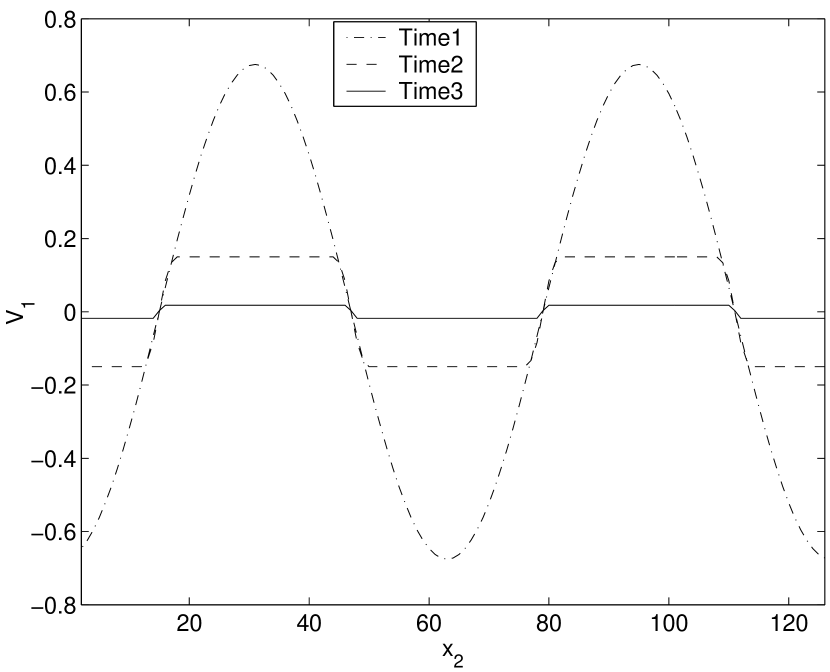
Figure 2: Evolution of $v_{1}(x_{2},t)$.

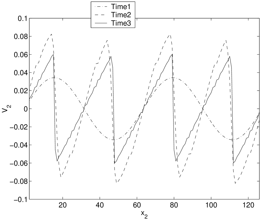
Figure 3: Evolution of $v_{2}(x_{2},t)$.

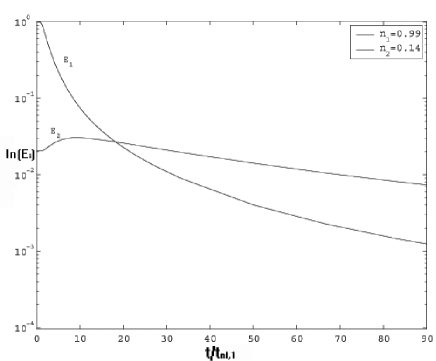
Figure 4: Evolution of the velocity components energies.

For the periodic structure (17) when $k_{1}\gg k_{2}$ we have that the plane wave $\psi_{0}\cos(k_{1}x_{1})$ is modulated by large scale function $M({\bf x})=\cos{(k_{1}x_{1})}$ eq. (29). The initial perturbation in this case is periodic structure with periods $l_{1}=2\pi/k_{1}$ , $l_{2}=2\pi/k_{2}$ and $l_{1}\ll l_{2}$.

Before the nonlinear distortion of large scale component $t\ll t_{{\rm nl},2}=l_{2}/\sigma_{\psi}$ the evolution of structure take place like in general case of modulated wave eq. (29). The velocity component $v_{1}(x_{1},x_{2},t)$ is transformed into saw-tooth wave (Figure 2) and we have a fully depression of initial amplitude modulation of this component (Figure 2). The velocity component $v_{2}$ loss the periodic modulation over $x_{1}$ and $v_{2,0}(x_{1},x_{2},t)\simeq\psi_{0}|\cos{(k_{2}x_{2})}|{{}^{\prime}}_{x_{2}}$. The period of this component is twice less than the initial period (Figure 3) and the energy increases twice in compare with the initial energy. The behavior of the energy is shown on the Figure 4.

IV Evolution of anisotropic multidimensional Burgers turbulence

IV.1 The intermediate stage of evolution of anisotropic random field

In this section we will consider the intermediate stage of evolution of anisotropic random field in the two dimensional Burgers equation. Let us assume that the initial potential $\psi_{0}(x_{1},x_{2})$ is random and strong anisotropic field with the spatial scales $l_{1}\ll l_{2}$. The initial energy $E_{i}(t)=\langle v_{i}^{2}\rangle=\langle(\partial\psi/\partial{x_{i}})^{2}\rangle=\sigma_{\psi}/l_{i}^{2}$ of the velocity component $v_{1}$ is in this case much larger than the energy of the large scale component $v_{2}$ . We can introduce the nonlinear time of $i$-th component as $t_{{\rm nl},i}=l_{i}^{2}/\sigma_{\psi}$. For $t\ll t_{{\rm nl},2}$, the drift of the Lagrangian particles in direction $x_{2}$ is relatively small. Then one can assume $y_{2}=x_{2}$ in eq. (9) and consider the one-dimensional problem with the initial potential $\psi_{0}(y_{1},x_{2},t)$, where $x_{2}$ is a parameter.

Due to the condition $l_{1}\ll l_{2}$ the the first shock lines in the Lagrangian coordinates are on the points where $\partial{\psi}/\partial{y_{1}}$ has a minimum. In Eulerian space the are oriented primarily along the $x_{2}$ axis end its length in this direction increase in time. For $t\gg t_{{\rm nl},1}$ the velocity field $v_{1}(x_{1},x_{2},t)$ transforms to the sequence of triangular pulses

$$v_{1}(x_{1},x_{2},t) = \frac{x_{1}-y_{1,k}(x_{1},x_{2},t)}{t}\ ,$$

$${\rm for}\quad x_{1,k}^{s}<x_{1}<x_{1,k+1}^{s}\ ,$$

where $y_{1,k}(x_{1},x_{2},t)$ are the coordinates of absolute maximum of (9) over $y_{1}$ with $y_{2}=x_{2}$. The shock positions $x_{1,k}^{s}(x_{2},t)$ are

$$x_{1,k}^{s} = \frac{y_{1,k+1}+y_{1,k}}{2}+v_{k}t\ ,$$ (40)

$$v_{k} = \frac{\psi_{0}(y_{1,k}(x_{1},x_{2}),x_{2})-\psi_{0}(y_{1,k+1}(x_{1},x_{2}),x_{2})}{y_{1,k+1}(x_{1},x_{2})-y_{1,k}(x_{1},x_{2})}\ .$$

It means that at fixed $x_{2}$ the interval $x_{1,k}^{s}<x_{1}<x_{1,k+1}^{s}$ will be cover by the particles from small region near the Lagrangian point $y_{1,k}(x_{1},x_{2},t)$, and for the velocity component $v_{2}$ we get

$$v_{2}(x_{1},x_{2},t) = -\frac{\partial{\psi_{0}}(x_{1},x_{2})}{\partial{x_{2}}}|_{x_{1}=y_{1,k}(x_{2},t)}\ ,$$

$${\rm for}\quad x_{1,k}^{s}<x<x_{1,k+1}^{s}\ .$$

The velocity $v_{2}(x_{1},x_{2},t)$ doesn’t depend on $x_{1}$ between the shock-lines $x_{1,k}^{s}(x_{2})$ and $x_{1,k+1}^{s}(x_{2})$. The collision of the shocks in one-dimensional Burgers equation is now equal that at some point ${\bf x}_{*}$ two adjacent shock lines $x_{1,k}^{s}$ and $x_{1,k+1}^{s}$ touch each other. Then this point will be developed into new shock lines $x_{1,k}^{s,*}(x_{2})$ with the increasing in time length along axis $x_{2}$ and which on its ends transforms into lines $x_{1,k}^{s}$,$x_{1,k+1}^{s}$. Thus at $t_{n2,1}\gg t\gg t_{{\rm nl},1}$ the velocity field has a cellular structure, the border $x_{1,k}^{s}(x_{2})$ of the cells are describing by the equation (40), the velocity component $v_{1}({\bf x})$ has an universal structure (IV.1). Velocity component $v_{2}({\bf x})$ inside the cell does not depend on $x_{1}$ and along the axis $x_{2}$ reproduced the behaviour of $v_{2}$ along the line $x_{1}=y_{1,k}(x_{2},t)$ eq. (IV.1). The evolution of the potential is plotted on Figure 5.

The statistical problems of the velocity component $v_{1}$ at this stage are similar to the properties of one-dimensional Burgers turbulence. The integral scale $L_{1}(t)$ and the energy $E_{1}(t)\sim\sigma_{\psi}/t$ of the component $v_{1}$ are described by the expressions (I), where $\sigma_{\psi}$ is the variance of initial two-dimensional potential $\psi_{0}$ and $l_{0}=l_{1}$ is the integral scale of $v_{1}$ component $L_{1}=\sigma_{\psi}/\sigma_{v_{1}}$. Due to the merging of the shock lines the integral scale of the turbulence along the axis $x_{1}$ increases with time $L_{1}(t)\sim(t\sigma_{\psi})^{1/2}$ and at $t\sim t_{{\rm nl},2}$, when $L_{1}(t)\simeq l_{2}$ and $E_{1}(t)\simeq E_{2}(0)$ we need to take into account the nonlinear distortion along the axis $x_{2}$. At $t\gg t_{{\rm nl},2}$ the potential and velocity fields have a universal isotropic and self-similar structure inside the cells: eq.(13), (14). The boundary of the cells on this stage degenerate into straight lines (planes, in three dimensional case). The multiply merging of the cell will leads to the establishment of statistical self-similarity and isotropization of the field. In the next section we will show how the statistical properties of the isotropic multidimensional Burgers turbulence are connected with the parameter of anisotropic initial perturbation.

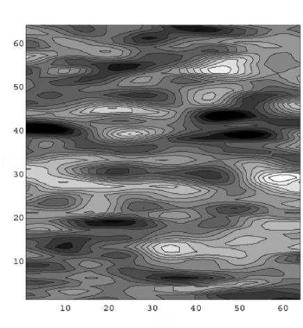
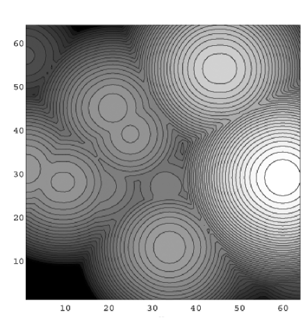
Figure 5: Evolution of potential. (Initial potential and stage of isotropization)

IV.2 Isotropisation of the multidimensional Burgers turbulence

The statistical properties of the Burgers velocity field $\bf v$ (equation (10)) in the limit $\nu\rightarrow 0$ are determined by the statistical properties of the absolute maximums coordinate $\bf{y}(\bf{x},t)$ of the function (9). In one-dimensional case the problem of the absolute maximum is reduced to the problem of the crossing the random signal $\psi_{0}(x)$ by the non homogeneous function $(x-y)^{2}/2t+H$. The asymptotic behaviour of the field at large $t$ is determined by the maximum which amplitude is higher than the variance of the initial potential. That’s why one can use some results of the theory of extremal processes LLR83 ; GMS91 ; MSW95 . In multidemensional case the problem of the peaks statistic of the Gaussian field is rather well known for the isotropic and homogeneous field BBKS86 . But for the Burgers turbulence we need to find the statistical properties of the absolute maximum of the scalar non homogeneous and anisotropic field $\Phi({\bf x},{\bf y},t)$. In paper GM2003 it was shown that at large $t$ this problem is reduced to the problem of the finding of the statistical properties of extremum of random field $\psi_{0}({\bf x})$ which value is much greater than their variance $\sigma_{\psi}$.

Let us assume the initial potential $\psi_{0}({\bf x})$ is random Gaussian field and it’s correlation function may be used in the following form

$$\langle\psi_{0}({\bf x})\psi_{0}({\bf x}+{\bf z})\rangle=B_{\psi}({\bf z})=\sigma_{\psi}^{2}\prod_{i=1}^{d}{R_{i}(z_{i})},$$ (42)

$$R_{i}(z_{i})=1-\frac{z_{i}^{2}}{2!l_{0,i}^{2}}+\frac{z_{i}^{4}}{4!l_{1,i}^{4}}+....$$ (43)

We assume also that the correlation function decreases rather fast at large distances; $B_{\psi}(|{\bf z}|>l_{st})\simeq 0$. Then the Gaussian initial field $\psi_{0}({\bf x})$ in the points $|{\bf x_{1}}-{\bf x_{2}}|>l_{st}$ is statistically independent.

In the limit of vanishing viscosity we have ”maximum representation” for the potential eq. (9). In this solution the velocity field ${\bf v}({\bf x},t)$ eq. (10) is determined by the coordinate $\bf y$ of the absolute maximum of function $\Phi({\bf x,y},t)$. Let $Q(H,\triangle V_{k})$ denote the cumulative probability and $W_{max}(H,\triangle V_{k})$ denote the probability density of the absolute maximum in elementary volume $\triangle V_{k}$

$$Q(H,\triangle V_{k})=Prob(\Phi<H,{\bf y}\in\triangle V_{k}),$$ (44)

$$W_{max}(H,\triangle V_{k})=Q^{\prime}_{H}(H,\triangle V_{k}).$$ (45)

Here we introduce the elementary volume $\triangle V_{k}$ which scale is much greater than $l_{st}$, but much smaller than the integral scale of turbulence $L(t)$. The probability for the absolute maximum to be contained between $H_{1}$ and $H_{1}+\triangle H_{1}$ with the coordinate ${\bf y}({\bf x},t)\in\triangle V_{k}$ equals to that one for the absolute maximum $H_{1}\in(H,H+\triangle H)$ to lie in $\triangle V_{k}$ and to be less than $H$ in magnitude for outer intervals $\overline{\triangle V}_{k}$

$$Prob \displaystyle({\bf y}\in\triangle V_{k},H\in[H_{1},H_{1}+\triangle H])$$ (46)

$$=W_{max}(H,\triangle v_{k})\triangle HQ(H,\overline{\triangle V}_{k}).$$

Here we propose that the absolute maximums are statistically independent in the intervals $\triangle V_{k}$ and $\overline{\triangle V}_{k}$ . The probability for coordinate ${\bf y}({\bf x},t)$ to fall into $\triangle V_{k}$ can be obtained by the integration of (46) with respect of H

$$Prob({\bf y}\in\triangle V_{k})=\int{W_{max}(H,\triangle V_{k})Q(H,\overline{\triangle V}_{k})}dH.$$ (47)

After the integration of (47) by parts we have

$$Prob({\bf y}\in\triangle V_{k})=\int{N(H,\triangle V_{k})Q^{\prime}_{H}(H)}dH,$$ (48)

where Q(H) is the integral distribution function of absolute maximum in the whole space. In Appendix in GM2003 it was shown that for large $H$ the integral distribution function

$$Q(H,\triangle V_{k})=\exp{\left(-N(H,\triangle V_{k})\right)}$$ (49)

is determined by the mean number of extremum $N(H,\triangle V_{k})$ with value larger than $H$.

Let us first consider the statistical properties of the extremum of the homogeneous random field $\psi_{0}({\bf x})$. It’s known that for the smooth fields the number of crossing some higher level asymptotically tends to the number of maximum and number of extremum. It means, that all the peaks above some high lever have only one extremum, which is the maximum of this peak. Thus we will consider first the properties of extremum of the field $\psi_{0}({\bf x})$. Using these properties of $\delta$-function one can obtain for the mean number $N(H;V)=\langle N_{exp}\rangle$ of extremum with the value greater than $H$ in some volume $V$

$$N(H;V)=\left\langle\int_{V}\delta(\nabla\psi_{0})|J(a_{ij})|E(\psi_{0}-H)d{\bf x}\right\rangle.$$ (50)

Here $E(s)$ is a unit function, and $J$ is the Jacobian of transformation

$$J(a_{ij})=|a_{ij}|,\;\;\;a_{ij}=\frac{\partial{\psi_{0}({\bf x})}}{\partial{x_{i}}\partial{x_{j}}}.$$ (51)

For the homogeneous field $\psi_{0}({\bf y})$ one can introduce the density of extremum as $n_{ext}(H;V)=N(H)/V$. The density of $n_{ext}$ in this case is determined by the joint probability distribution function of the $\psi_{0}$, their gradient $v_{i}=\partial{}\psi_{0}/\partial{x_{i}}$ and tensor $a_{ij}=\partial{\psi_{0}}/\partial{x_{i}}\partial{x_{j}}$. For the homogeneous Gaussian field $W_{\psi_{0},v_{i},a_{ij}}=W_{v}(v_{i})W_{\psi_{0},a_{ij}}(\psi_{0},a_{ij})$ and from eq. (50) we have for the density of extremum

$$n_{ext}(H)=W_{v}(0)\int_{H}^{\infty}dS\int da_{ij}J(a_{ij})W_{\psi_{0},a_{ij}(S,a_{ij})}.$$ (52)

For the Gaussian field the p.d.f. of the field $\psi_{0}({\bf x})$ and it’s derivative are determined by the correlation function of $\psi_{0}({\bf x})$ eq. (42). In equation (52) we will integrate over the conditional probability $W_{con}(a_{ij}/S)=W(a_{ij},S)/W_{\psi_{0}}(S)$ and will get

$$n_{ext}=W_{v}(0)\int_{H}^{\infty}dSW_{\psi_{0}}(S)\int da_{ij}J(a_{ij})W_{con}(a_{ij}/S).$$ (53)

Using the properties of Gaussian variables one can receive that the conditional expected value of $a_{ij}$ is $\langle a_{ij}\rangle_{con}=S\langle a_{ij}S\rangle/\sigma_{\psi}^{2}$. In the problem of the Burgers turbulence at large time the asymptotic of $n_{ext}$ of high value $H$ is important. Thus in conditional averaging we have

$$\langle J(a_{ij})\rangle_{con}\simeq J(\langle a_{ij}\rangle_{con})\simeq\prod_{i=1}^{d}\langle a_{ii}\rangle_{con}=\frac{S^{d}}{l_{0,eff}^{2d}}.$$ (54)

Here we introduce the effective length $l_{0,eff}$

$$l_{0,eff}^{d}=\prod_{i=1}^{d}l_{0,i}$$ (55)

and take into account that $\langle a_{ii}^{2}\rangle=\sigma_{\psi}^{2}/l_{0,i}^{4}$. Finally we obtain from equations (53),(54) for the density of extremum the following expression

$$n_{ext}(H) = W_{v}(0)\int^{\infty}_{H}dSW_{\psi_{0}}(S)\frac{S^{d}}{l_{eff}^{2d}}$$ (56)

$$= \frac{1}{(2\pi)^{\frac{d+1}{2}}l_{eff}^{d}}\int_{H/\sigma_{\psi}}^{\infty}S^{d}e^{-S^{2}/2\sigma_{\psi}^{2}}dS$$

$$\simeq \left(\frac{H}{\sigma_{\psi}}\right)^{d-1}\frac{1}{(2\pi)^{\frac{d+1}{2}}l_{eff}^{d}}e^{-H^{2}/2\sigma_{\psi}^{2}}.$$

Thus from equation (56) one can receive that the mean number of the extremum of anisotropic field $\psi_{0}(\bf{x})$ is determined by some effective spatial scale $l_{eff}$, which is geometrical mean of spatial scale $l_{0,i}$. For the relatively large $H$ the density of extremum (56) is equal to the density of events that the random field $\psi_{0}({\bf x})$ is over the $H$.

For the homogeneous field $N(H;V)=Vn_{ext}(H)$, where $n_{ext}(H)$ is described by the equation (56). For the nonhomogeneous field, even in one-dimensional case, the expression for $N$ is more complicated. We assume that the nonhomogeneous field is $\Phi({\bf x})=\psi_{0}({\bf x})-\alpha({\bf x})$ and $\alpha({\bf x})$ is a smooth function in scale of $\psi_{0}({\bf x})$. Then in a quasistatic approximation one can receive for the mean number of events $N(H;V)$ that $\Phi({\bf x})>H$ in a volume $V$ the following expression

$$N(H;V)=\int_{V}{n_{ext}(H+\alpha({\bf x}))}dV,$$ (57)

where $n_{ext}(H)$ is determined by the expression (56) and is the density of extremum of the statistically homogeneous function $\psi_{0}({\bf x})$.

At large time the paraboloid $\alpha=({\bf x}-{\bf y})^{2}/2t$ in equation (9) is a smooth function in the scale of the initial potential. Then for the mean number of maximums one can use quasi-static approximation eq. (57) and

$$Q(H) = \exp{\left(-N_{\infty}(H)\right)}$$ (58)

$$N_{\infty}(H) = \int{n_{ext}\left(H+\frac{(\bf{x}-\bf{y})^{2}}{2t}\right)}dV.$$ (59)

Here $N_{\infty}(H)$ is the mean number of extremum of $\Phi({\bf x,y},t)$ in the hole space with magnitude greater then $H$ and $n_{ext}(H)$ is the density of the number of extremum of the initial homogeneous potential $\psi_{0}({\bf x})$ with value greater then $H$ . For $H\gg\sigma_{\psi}$ the density $n_{ext}(H)$ is determined by the expression (56) and we have

$$N_{\infty}(H) = \frac{1}{(2\pi)^{(d+1)/2}l_{eff}^{d}}$$ (60)

$$\int{\left(\frac{H}{\sigma_{\psi}}\right)^{d-1}e^{-(H+{\bf y}^{2}/2t)^{2}/2\sigma_{\psi}^{2}}}d{\bf y}$$

$$\simeq \left(\frac{H}{\sigma_{\psi}}\right)^{d-1}\frac{1}{\sqrt{2}\pi}\left(\frac{\sigma_{\psi}^{2}t}{Hl_{eff}^{2}}\right)^{d/2}e^{-H/2\sigma_{\psi}^{2}}.$$

In equation (58) we integrate over the infinite space, but the effective volume $(\sigma_{\psi}^{2}t/Hl_{eff}^{2})^{d/2}$ is determined by the paraboloid term in equation ( 58). Now the effective number of independent local maximum in initial perturbation is $N_{max}\sim(\sigma_{\psi}t/l_{eff}^{2})^{d/2}$ and increases with time. When $N_{max}\gg 1$ we can introduce the dimensionless potential $h$ as follows

$$H=h\sigma_{\psi},\;\;\;h=h_{0}(1+z/h_{0}^{2}),$$ (61)

where $h_{0}=H_{0}\sigma_{\psi}$ and $H_{0}$ is the solution of the equation $N(H_{0})=1$

$$h_{0}\simeq d^{1/2}\left(\log{\frac{\sigma_{\psi}t}{l_{eff}^{2}(2\pi)^{1/d}}}\right)^{1/2},\;\;\langle\psi({\bf x},t)\rangle\simeq\sigma_{\psi}h_{0}.$$ (62)

Thus we have a logarithmic growth of mean potential. The dimensionless potential has double exponential distribution

$$Q(z) = \exp{(-\exp{(-z)})}\ ,$$

$$Q_{h}(h) = \exp{(-\exp{(-(h-h_{0})h_{0})}},$$ (63)

One can see that for $t\gg t_{\rm nl}=l_{eff}^{2}/\sigma_{\psi}$ we have $N_{max}\gg 1$ and the integral distribution of absolute maximum is concentrated in narrow region $\triangle H/H\simeq\sigma_{\psi}^{2}/H_{0}^{2}\ll 1$ near $H_{0}$. Using this fact one can get from (48) the probability distribution of the maximums coordinate

$$W({\bf y},{\bf x},t)=\frac{1}{\sqrt{2\pi L^{2}(t)}}\exp{-\frac{({\bf x}-{\bf y})^{2}}{2L^{2}(t)}},$$ (64)

where

$$L(t)=\left(\frac{\sigma_{\psi}t}{h_{0}}\right)^{1/2}=(\sigma_{\psi}t)^{1/2}d^{-1/4}\left(\log{\frac{\sigma_{\psi}t}{l_{eff}^{2}(2\pi)^{1/d}}}\right)^{-1/4}$$ (65)

is the integral scale of the turbulence. From equation (10),(64) we see that the one-dimensional probability distribution of the velocity field is Gaussian and isotropic. For the energy of each component we have

$$E_{i}(t)=\sigma_{v,i}^{2}=\frac{L^{2}(t)}{t^{2}}=\left(\frac{\sigma_{\psi}}{t}\right)d^{-1/2}\left(\log{\frac{\sigma_{\psi}t}{l_{eff}^{2}(2\pi)^{1/d}}}\right)^{-1/2}.$$ (66)

Thus for the anisotropic initial field there’s the isotropisation of the turbulence.

For the multi-dimensional Burgers turbulence the two-dimensional probability distribution, correlation function and energy spectrum where found in GurbatovSaichev1984 ; GMS91 using so called “cellular” model. In this model is assumed that in different elementary volumes the initial potential are independent and that the potential has a Gaussian distribution. In this model there’s a free parameter $\triangle$ which is the size of the elementary cell. In the present work we consider a continuous initial random potential field with given correlation function (42),(43). The procedure for calculation of the two-point probability distribution function is nevertheless similar to that one used in GurbatovSaichev1984 ; GMS91 . It’s easy to show that for the two-point P.D.F. we have the same expression as obtained in GMS91 for the cell model, only the size of the cell $\triangle$ we used to change with the effective spatial scale $l_{eff}$. The effective spatial scale $l_{0,eff}$ (55) is determined by the scales $l_{0,i}$ of initial correlation function (42). For the two-point P.D.F., correlation function and energy spectrum we also have the self-similarity and isotropisation at large times. In particular for the normalized longitudinal and transverse correlation function of the velocity field $\tilde{\bf v}={\bf v}/\sigma_{v,i}$ we have

$$\tilde{B}_{LL}(\tilde{x})=\langle\tilde{v}_{1L}\tilde{v}_{2L}\rangle={d\over d\tilde{x}}\left(\tilde{x}P(\tilde{x})\right),$$ (67)

$$\tilde{B}_{NN}(\tilde{x})=\frac{1}{2}\langle\tilde{v}_{1N}\tilde{v}_{2N}\rangle=P(\tilde{x}),$$ (68)

where $\tilde{x}=x/L(t)$ and

$$P(\tilde{x})=\frac{1}{2}\int_{-\infty}^{\infty}{dz\over g\left({\tilde{x}+z\over 2}\right)\exp\left[{(\tilde{x}+z)^{2}\over 8}\right]+g\left({\tilde{x}-z\over 2}\right)\exp\left[{(\tilde{x}-z)^{2}\over 8}\right]}$$ (69)

$$g(z)\equiv\int_{-\infty}^{z}e^{-{s^{2}\over 2}}\,ds.$$ (70)

It may be shown that the function $P(\tilde{x})$ is the probability of having no shock within an Eulerian interval of length $\tilde{x}L(t)$. As far as potential isotropic field are concerned, the normalized energy spectrum $e(k)$ is formulated via a one-dimensional spectrum $e_{NN}(k)$ of the transverse component. The energy spectrum $E_{v}(k,t)$ is isotropic and self-similar

$$E(k,t)=\frac{L^{3}(t)}{t^{2}}\tilde{E}(kL(t)).$$ (71)

At large wave number $k$ the discontinuity initiation leads to the power asymptotic behaviour $E(k,t)\sim k^{-2}$. At small wave number is also has the universal behaviour

$$E(k,t)=k^{d+1}\frac{L^{4+d}(t)}{t^{2}}\sim k^{d+1}t^{d/2},$$ (72)

which has do with the nonlinear generation of low-frequency component. In particular for the three-dimensional turbulence we have $E(k,t)\sim k^{4}t^{3/2}$. For the large, but finite Reynolds numbers, the ”shocks” have a finite width $\delta\sim\nu t/L(t)$ and relative width increases slowly with time $\delta/L(t)\sim\left(\log{(\sigma_{\psi}t/l_{eff}^{2})}\right)^{1/2}$. Thus at very large time we have a linear stage of evolution.

IV.3 The linear stage of evolution of Burgers turbulence

Let us now consider the linear stage of evolution of random field, when the potential $\psi({\bf x},t)$ and the velocity field ${\bf v}({\bf x},t)$ eq.(16) are linearly connected with the solution $u({\bf x},t)$ of the linear diffusion equation eq. (7). Here $u({\bf x},t)$ are the relative fluctuations of the field $U({\bf x},t)$ eq. (15). Introduce the spectral density of the field $u({\bf x},t)$ as

$$E_{u}({\bf k},t)=\frac{1}{(2\pi)^{d}}\int B_{u}({\bf z},t)e^{i({\bf kz})}d{\bf z},$$ (73)

where $B_{u}({\bf z},t)=\langle u({\bf z},t)u(0,t)\rangle$ is a correlation function of relative fluctuation field $\tilde{U}({\bf x},t)$. The evolution of the spectral density $E_{u}({\bf k},t)$ and variance $\sigma_{u}^{2}(t)$ of $u$ are described by the equations

$$E_{u}({\bf k},t)=E_{u0}({\bf k})e^{-2\nu k^{2}t},\;\;E_{u0}({\bf k})=E_{u}({\bf k},0)$$ (74)

$$\sigma_{u}^{2}(t)=\int{E_{u0}({\bf k})e^{-2\nu k^{2}t}}d{\bf k}\;\;.$$ (75)

For the homogeneous Gaussian initial potential $\psi_{0}({\bf x})$ we have from eq. (6)

$$E_{u0}({\bf k})=\frac{1}{(2\pi)^{d}}\int\left[\exp\left(\frac{B_{\psi}({\bf z})}{4\nu^{2}}\right)-1\right]e^{i({\bf kz})}d{\bf z}\;\;,$$ (76)

where $B_{\psi}({\bf z})$ is the correlation function of initial potential $\psi_{0}({\bf x})$. The condition of Burgers turbulence entering the linear regime is $t\gg t_{lin}$, where $t_{lin}$ is determined from the equation $\sigma_{u}^{2}(t_{lin})\simeq 1$ . From eq. (74) one can see, that the old-age behaviour of the scalar field $u$ and consequently the velocity field ${\bf v}$ will be determined by the behaviour of the energy spectrum $E_{u0}({\bf k})$ at small wave numbers ${\bf k}$. When the correlation function of initial potential $\psi_{0}({\bf x})$ may be represented in the form (42) at small ${\bf\rho}$ and $B_{\psi}(|\rho|>l_{st})\simeq 0$, then from eq. (76) we have, that the spectrum $E_{u0}({\bf k})$ at $k\ll{\rm Re}_{0}/l_{eff}$ is flat and

$$E_{u0}({\bf k}=0)=D_{u}\simeq\frac{1}{(2\pi)^{d/2}}(l_{eff}/{\rm Re}_{0})^{d}\exp{\left({\rm Re}_{0}^{2}\right)}\;\;,$$ (77)

where $l_{eff}$ is determined by equation (55). The spectrum of the field $u$ at large time is isotropic and has an universal form

$$E_{u}({\bf k},t)=D_{u}e^{-2\nu k^{2}t}\;\;\,$$ (78)

and consequently isotropic is the velocity field GurbatovSaichev1984 ; GMS91 ; AMS94 . The energy of each component decays as $E_{i}(t)\sim D_{u}(\nu t)^{-(d+2)/2}$.

Consider now the case when the initial potential has a correlation function (42) at small ${\bf x}$ and has a long correlation at large ${\bf x}$ AMS94

$$B_{\psi}({\bf x})=\sigma_{\psi}^{2}\left(|{\bf x}|/l_{long}\right)^{-\alpha}F_{B}({\bf x}/|{\bf x}|),\;\;\alpha>0.$$ (79)

Here the function $F_{B}({\bf x}/|{\bf x}|)$ describes the anisotropy of correlation function at long distances. If $\alpha>d$ the evolution of the spectrum of $u$ (eq.78) and the velocity ${\bf v}$ will be the same as in absents of long correlation AMS94 . At $0<\alpha<d$ the energy spectrum of initial potential has a singularities at small wave number

$$E_{\psi}({\bf k})=\sigma_{\psi}^{2}l_{long}^{\alpha}|{\bf k}|^{\alpha-d}F_{E}({\bf k}/|{\bf k}|),\;\;0<\alpha<d,$$ (80)

where the function $F_{E}({\bf k}/|{\bf k}|)$ is determined by the function $F_{B}({\bf x}/|{\bf x}|)$ and describes the anisotropy of potential spectrum at small wave number. It was shown AMS94 that in this case we have the conservation of anisotropy at linear stage and asymptotic behaviour of the spectrum of $u$ is determined by the equation (74) where

$$E_{u}({\bf k})=E_{\psi}({\bf k})/(4\nu)^{2}={\rm Re}_{0}^{2}l_{long}^{\alpha}|{\bf k}|^{\alpha-d}F_{E}({\bf k}/k)\;\;.$$ (81)

For the velocity spectrum it means that it reproduced the initial spectrum of velocity at small wavenumber multiplied by the exponential factor $\exp{(-2\nu k^{2}t)}$. These results was formulated AMS94 for the correlation function of velocity fields. In paper AMS94 also was shown that asymptoticly the velocity field has Gaussian distribution. But the transformation processes to the linear stage are not trivial and may be estimated on base of spectral representation. The behaviour of the spectral density of the field $u$ at small wave number ${\bf k}$ is determined by the tail of correlation function $B_{\psi}({\bf x})$ (79) and from eq. (76) we have that the spectrum is described by the equation (81). But with the increasing of the module of wave number $k$ the power anisotropic spectrum transformed to the flat spectrum (77). The wave number $k_{af}$ where this transformation take place may be estimated from the condition that at $k\simeq k_{af}$ these spectrum are the same order and we have

$$k_{af}\simeq{\rm Re}_{0}^{(d+2)/(d-\alpha)}\left(\frac{l_{long}^{\alpha}}{l_{eff}^{d}}\right)^{1/(d-\alpha)}e^{-{\rm Re}_{0}^{2}/(d-\alpha)}.$$ (82)

The condition of Burgers turbulence entering the linear regime is determined from the equation $\sigma_{u}^{2}(t_{lin})\simeq 1$. The main contribution in the variance $\sigma_{u}^{2}(t)$ eq. (75) we have from the flat spectrum eq.(77). The wave number $k_{lin}\simeq(\nu t_{lin})^{-1/2}$ is

$$k_{lin}\simeq({\rm Re}_{0}/l_{eff})e^{-{\rm Re}_{0}^{2}/d}.$$ (83)

Thus for the ratio of this two critical wave numbers we have

$$k_{af}/k_{lin}\simeq{\rm Re}_{0}^{(\alpha+2)/(d-\alpha)}\left(\frac{l_{long}}{l_{eff}}\right)^{1/(d-\alpha)}e^{-{\rm Re}_{0}^{2}\alpha/d(d-\alpha)},$$ (84)

and for the large initial Reynolds number $k_{af}\ll k_{lin}$. From the equation $\sigma_{u}^{2}(t_{lin})\simeq 1$ we have that $t_{lin}\simeq t_{\rm nleff}{\rm Re}_{0}^{-1}\exp{(2{\rm Re}_{0}^{2})}$ and is extremely large in compare with the effective nonlinear time $t_{\rm nleff}\simeq l_{eff}^{2}/\sigma_{\psi}$. It is easy to see from (82)) that the time of “isotropisation” $t_{iso}\simeq\nu k_{af}^{2}$ is much greater then the nonlinear time $t_{iso}\sim t_{\rm nleff}e^{2{\rm Re}_{0}^{2}\alpha/d(d-\alpha)}$ and this difference increaces when the index $\alpha$ is near the critical value $\alpha\simeq d$.

V Discussion and conclusion

Let us now discuss the evolution of the turbulence in presence of anisotropy at small (42) or large (79) spatial scales. In initial perturbation the energy of the velocity component is $\sigma_{\psi}^{2}/l_{0,i}^{2}$ and is greater for the small scales $l_{0,i}$. At the initial stage the scale of the turbulence in this direction increases faster then in others and we have primarily the energy decay primarily of this component (see SectionIV.1). After the time $t$ is greater the of the nonlinear time of the the component with the largest scale $t_{{\rm nl},i}=\max l_{0,i}^{2}/\sigma_{\psi}$ we have the isotropisation of turbulence in the scales in order of the integral scale of turbulence $L(t)$ (65). In Section IV.2 we consider the situation in absence of long scale correlation. But based on the results of one dimensional case GSAFT97 we may suggest that there are no influence a long scale correlation on the evolution of the energy. Nevertheless we still have conservation of anisotropy at large scales $|{\bf x}|\gg L(t)$ (79). In the spectral representation we have the conservation of the inital spectrum and anysotropy at small wave number, but at $k\sim k_{s}(t)\sim t^{-p}$ the initial spectrum trasformes into selfsimular spectrum (71) with the universal behaviour $E(k,t)\sim k^{(d+1)}$ eq. (72) at $kL(t)<1$. Let us define an energy wavenumber $k_{L}(t)=L^{-1}(t)\sim(t\sigma_{\psi})^{-1/2}$, which is roughly the wavenumber around which most of the kinetic energy resides. Hence, the switching wavenumber $k_{s}(t)$ goes to zero much faster than the energy wavenumber. Taking into account the finite viscosity we have that after the $t\gg t_{lin}\simeq t_{\rm nleff}{\rm Re}_{0}^{-1}\exp{(2{\rm Re}_{0}^{2})}$ the nonlinear evolution of the spectrum is frozen and only the linear decays of the small scales is significant (74). The frozen spectrum of the velocity potential has a critical wavenumber $k_{af}$ bellow which the spectrum is anisotropic and reproduce the initial spectrum, and at $k>k_{af}$ is flat eq.(77) . Thus at $t_{af}\gg t\gg t_{lin}$ this part of the spectrum will play the dominate role in the evolution of the velocity spectrum, consequently the energy of all velocity component are equal. At $t\gg t_{af}$ the spectrum of the velocity will be reproduced the small scale part of the initial velocity spectrum multiplied by the exponential factor (74), and we have finally the anisotropic field.

Acknowledgments. We have benefited from discussion with U. Frisch, A. Saichev, A. Sobolevskii. This work was supported by Grants : RFBR-08-02-00631-a, SS 1055.200.2. S. Gurbatov thanks the French Ministry of Education, Research and Technology for support during his visit to the Observatoire de la Côte d’Azur.

References

- (1) G.B. Whitham, Linear and Nonlinear Waves (Wiley, New York, 1974).
- (2) O.V. Rudenko and S.I. Soluyan Nonlinear acoustics (Pergamon Press, New York, 1977).
- (3) S.N. Gurbatov, A.N. Malakhov, and A.I. Saichev Nonlinear Random Waves and Turbulence in Nondispersive Media: Waves, Rays, Particles (Manchester University Press,1991).
- (4) W.A. Woyczynski, Burgers–KPZ Turbulence. Gottingen Lectures (Springer-Verlag, Berlin,1998).
- (5) U. Frisch, J. Bec Burgulence.Les Houches 2000: New Trends in Turbulence,pp. 341-383 (Springer EDP-Sciences,2001); arXiv:nlin/0012033v2 [nlin.CD]
- (6) J.Bec, K.Khanin, Physics Reports, 447, Issue 1-2, 1 (2007).
- (7) J.M. Burgers, Kon. Ned. Akad. Wet. Verh. 17, 1 (1939)
- (8) J.M. Burgers The Nonlinear Diffusion Equation. (D. Reidel, Dordrecht, 1974).
- (9) U. Frisch U. Turbulence: the Legacy of A.N. Kolmogorov (Cambridge University Press,1995).
- (10) R. Kraichnan, Phys.Fluids Mech. 11, 265 (1968).
- (11) A. Chekhlov and V. Yakhot, Phys. Rev. E 52, 5681 (1995)
- (12) A. M. Polyakov, Phys. Rev. E 52, 6183 (1995).
- (13) W. E, K. Khanin, A. Mazel, and Ya. G. Sinai, Phys. Rev. Lett. 78, 1904 (1997).
- (14) S.A. Boldyrev, Phys. Rev. E 59, 2971 (1999)
- (15) J. Davoudi, A.A. Masoudi,M.R.R., Tabar, A.R. Rastegar, F. Shahbazi, Phys. Rev. E 63, 6308, (2001).
- (16) S.N. Gurbatov, and A.I. Saichev, Radiophys. Quant. Electr. 27, 303 (1984).
- (17) S.N. Gurbatov, A.I. Saichev, and S.F. Shandarin, Month. Not. R. astr. Soc. 236, 385 (1989).
- (18) S.F. Shandarin and Ya.B. Zeldovich, Rev. Mod. Phys. 61, 185 (1989)
- (19) M. Vergassola, B. Dubrulle, U. Frisch, and A. Noullez, Astron. Astrophys. 289, 325 (1994). 11
- (20) A. Andrievsky, S. Gurbatov and A. Sobolevsky, JETP. 104(10), 887 (2007)
- (21) A.-L. Barabási and H.E. Stanley Fractal Concepts in Surface Growth (Cambridge University Press, 1995).
- (22) E.A.Kuznetzov, S.S.Minaev, Phys. Let. A 221, 187, (1996).
- (23) M. Kardar, G. Parisi and Y.C. Zhang Phys. Rev. Lett. 56, 889 (1986).
- (24) J.–P. Bouchaud, M. Mézard and G. Parisi, Phys. Rev. 52, 3656 (1995).
- (25) Z.S. She, E. Aurell and U. Frisch, Commun. Math. Phys. 148, 623 (1992).
- (26) L. Frachebourg, L. and Ph.A. Martin, J. Fluid Mechanics, 417, 323 (2000).
- (27) S. Albeverio., A.A. Molchanov, and D. Surgailis, Prob. Theory Relat. Fields 100, 457 (1994)
- (28) S.E. Esipov, and T.J. Newman, Phys. Rev. E 48, 1046 (1993)
- (29) S.E. Esipov Phys. Rev. E 49, 2070 (1994)
- (30) T.J. Newman, Phys. Rev. E 55, 6988 (1997).
- (31) S.N. Gurbatov, Phys. Rev. E 61, 2595 (2000).
- (32) S. Kida, J. Fluid Mech. 93, 337 (1979).
- (33) S.N. Gurbatov and A.I. Saichev, Sov. Phys. JETP 80, 589 (1981).
- (34) J.D. Fournier and U.Frisch J. Méc. Théor. Appl. (France) 2, 699 (1983).
- (35) S.A. Molchanov, D. Surgailis and W.A. Woyczynski Comm. Math. Phys.168, 209 (1995).
- (36) S.N. Gurbatov, S.I. Simdyankin, E. Aurel, U. Frisch, and G.T. Tóth, J.Fluid Mech. 344, 339 (1997).
- (37) A.Noullez, S.N. Gurbatov, E. Aurel and S.I. Simdyankin, Phys. Rev. E 71, 056305 (2005).
- (38) E. Hopf, Comm. Pure Appl. Mech. 3, 201 (1951).
- (39) J.D. Cole, Quart. Appl. Math. 9, 225 (1951)
- (40) M.R. Leadbetter, G. Lindgren and H. Rootzen Extremes and Related Properties of Random Sequences and Processes. (Springer, Berlin, 1983)
- (41) J.M.Bardeen, J.R.Bond, N.Kaiser, A.S.Szalay, Astrophysical J. 304,15-61,(1986)
- (42) S.N. Gurbatov, A.Yu.Moshkov, JETP. 97(6), 1186, (2003).