Electrical probing of the spin conductance of mesoscopic cavities

Abstract

We investigate spin-dependent transport in multiterminal mesoscopic cavities with spin–orbit coupling. Focusing on a three-terminal setup we show how injecting a pure spin current or a polarized current from one terminal generates additional charge current and/or voltage across the two output terminals. When the injected current is a pure spin current, a single measurement allows to extract the spin conductance of the cavity. The situation is more complicated for a polarized injected current, and we show in this case how two purely electrical measurements on the output currents, give the amount of current that is solely due to spin-orbit interaction. This allows to extract the spin conductance of the device also in this case. We use random matrix theory to show that the spin conductance of chaotic ballistic cavities fluctuates universally about zero mesoscopic average and describe experimental implementations of mesoscopic spin to charge current converters.

Many recent theoretical, experimental and numerical investigations have explored possibilities to generate spin currents and accumulations in spin-orbit coupled diffusive Dya71 ; Sin04 ; Mur04 ; Ino04 ; Mis04 ; Ada05 ; Kat04 ; Wun05 ; Sai06 ; Sch05 ; Rai05 ; Ren06 ; Val06 ; Ada07 and ballistic Bar07 ; Nik05 ; Naz07 ; Kri08 systems. The main focus of this field of spin-orbitronics is on purely electrostatic generation of spin currents via application of charge currents and/or voltage biases at appropriate lead contacts to the device. The amount of spin current generated by a given bias defines a spin conductance $G^{(s)}$ characterizing the spin generation efficiency of the device. Although $G^{(s)}$ is theoretically convenient, no realistic setup to experimentally probe it has been proposed to date. Such a setup is highly desirable for ballistic mesoscopic cavities, which typically feature relatively high spin conductances Bar07 ; Kri08 . This property is however not sufficient to make them good candidate components for low-power spintronic devices because of the relatively large mesoscopic fluctuations exhibited by their spin conductance Bar07 . Originating from the phase coherence of spin transport, these fluctuations are beyond the existing measurement proposals which are based on theories describing ensemble averaged diffusive transport of spins, assuming locally well defined spin accumulations Han04 ; Erl05 ; Ada06 . In this Letter, we propose to use spin-orbit coupled ballistic mesoscopic cavities as spin- to charge-current converters to experimentally analyze spin currents and spin accumulations in meso- and nanoscopic devices. We show how the spin conductance of such cavities can be directly measured from the amount of charge current they generate out of conventionally injected spin currents.

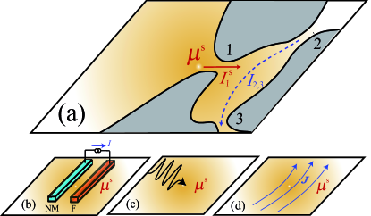
Figure 1: (Color online) (a) Three terminal ballistic quantum dot as a mesoscopic spin current to charge current converter. The output electrodes 2 and 3 are at the same fixed potential $V=0$, while the input electrode 1 is at potential $V_{1}$. Spins are injected into the dot from electrode 1. We argue that spin-orbit coupling can convert this spin current into a charge current across electrodes 2 and 3 (dashed blue arrow). We discuss three possible mechanisms for generating this spin current from a spin accumulation generated by (b) a ferromagnet, (c) polarized photons and (d) a charge current in the spin-orbit coupled reservoir 1. For these three mechanisms, it is straightforward to invert the spin accumulation, allowing to extract the spin conductance of the cavity from two measurements of the output charge current/voltage at opposite spin accumulations.

For simplicity, we choose the spin- to charge-current converter to be an open three-terminal quantum dot with spin-orbit coupling – this is sketched in Fig. 1a – though our discussion is straightforwardly generalized to multi-terminal cavities with any number of leads greater than two. The spin accumulation $\bm{\mu}^{(s)}$ (the components of that vector give the difference in chemical potential of different spin species along the corresponding spin direction) in a bulk electron reservoir generates a spin current $I_{1}^{(s)}$ injected into the dot from terminal 1 Ada07 . Spin-orbit coupling inside the dot acts on the pure spin part of this current in a manner similar to the inverse spin Hall effect Val06 – it converts it into either a transverse charge current, or a voltage difference between lead 2 and lead 3. This conversion differs however from the inverse spin Hall effect in that it is fully coherent and it couples different spin polarization. Measuring this charge current/voltage allows to extract the spin conductance of the cavity. We consider two types of measurements, defining two different spin conductances $G^{(s1)}$ and $G^{(s2)}$. In the first one, the voltage on terminal 1 is set such that $I_{1}^{(s)}$ is a pure spin current, without charge component, $I_{1}=0$. Then $I_{2}=-I_{3}$ are entirely due to the conversion of $I_{1}^{(s)}$ into a charge current, and the spin conductance of the cavity is defined as $G^{(s2)}_{j}\equiv I_{j}/|\bm{\mu}^{(s)}|$, $j=2,3$. In the second scenario, $I_{1}^{(s)}$ is a polarized current, accompanied by a net injection of charges into the dot, $I_{1}\neq 0$. To demonstrate the existence of a spin component in $I_{1}^{(s)}$, one thus needs to isolate that part of $I_{2}$ or $I_{3}$ that originates exclusively from the spin-orbit conversion of $I_{1}^{(s)}$. This is achieved by performing two measurements at reversed spin accumulation in 1, $\bm{\mu}^{(s)}\rightarrow-\bm{\mu}^{(s)}$, but fixed electrochemical potentials. As we show below, the difference in the two measured currents is solely due to the spin-orbit conversion of $I^{(s)}$. This defines the spin conductance of the cavity as $G_{j}^{(s1)}\equiv[I_{j}(\bm{\mu}^{(s)})-I_{j}(-\bm{\mu}^{(s)})]/2|\bm{\mu}^{(s)}|$, $j=2,3$, where the upper index refers to the type of measurement, while the lower index refers to the exit lead on which the current measurement is performed. In both instances, we show that $G^{(s)}_{j}$ exhibits mesoscopic fluctuations about zero average, under variation of the shape of the cavity or homogeneous changes in electrochemical potentials in all terminals.

There are various ways to generate spin accumulations and currents, most notably via spin injection from ferromagnetic components Lou06 or optical orientation optical , or via magneto-electric effects Ede90 ; Aro89 ; Duc08 ; Kat05 . Fig. 1b illustrate the first method, where a ferromagnetic lead, F, and a nonmagnetic lead, NM, form an $F\big{/}2DEG(2DHG)\big{/}NM$ junction with a two dimensional electron (hole) reservoir. Passing a current between F and NM injects spins into the reservoir. In Fig. 1c we sketch how spin polarization is generated via optical pumping with circularly polarized photons. Fig. 1d illustrates how a steady-state electronic current flowing in a two-dimensional $k$-linear spin-orbit coupled system generates a bulk spin accumulation Ede90 . In all cases, the spin accumulation, generated a distance shorter than the spin relaxation length but longer than the mean free path away from the point contact, diffuses to and flows through the ballistic cavity. Then, the ballistic processes connecting the spin injector part of the circuit with the cavity can be ignored and the reservoir can be viewed as having a well-defined spin accumulation $\bm{\mu}^{(s)}$.

We formalize our theory. An open quantum dot is coupled to three bulk reservoirs via ideal point contacts, each carrying $N_{i}$ open channels ($i=1,2,3$). We assume that spin-orbit coupling exists only inside the dot. Given that the dot and the reservoirs are made of the same material, this is justified when (i) the openings to the electrodes are small enough, that the spin-orbit time is shorter than the mean dwell time spent by an electron in the dot, and (ii) the accumulations in the reservoirs are generated a distant shorter than the spin-orbit length away from the dot. We follow the scattering approach to transport and start from the linear relation between currents and chemical potentials But86 ,

$$I_{i}^{(\alpha)}=\frac{e}{h}\sum_{\beta}(2N_{i}\delta_{\alpha\beta}-\mathcal{T}^{(\alpha\beta)}_{ii})\mu_{i}^{(\beta)}-\frac{e}{h}\sum_{j\neq i,\beta}\mathcal{T}^{(\alpha\beta)}_{ij}\mu_{j}^{(\beta)}.$$ (1)

Here, $\mu_{i}^{(0)}=eV_{i}$ ($V_{i}$ is the voltage applied to terminal $i$) and $\mu_{i}^{(\beta)}$ are the components of the spin accumulation vector $\bm{\mu}^{(s)}_{i}$, giving the difference in chemical potential between the two spin species along the corresponding axis, i.e. $\mu_{i}^{(z)}=\mu_{i}^{(\uparrow)}-\mu_{i}^{(\downarrow)}$, while $I^{(0)}_{i}\equiv I_{i}$ and $I_{i}^{(\alpha)}$ are the charge current and the components of the spin current vector, all evaluated in terminal $i$. We introduced the spin-dependent transmission probabilities

$$\mathcal{T}_{ij}^{(\alpha\beta)}=\sum_{m\in i,n\in j}{\rm Tr}[t_{mn}^{\dagger}\sigma^{(\alpha)}_{m}t_{mn}\sigma^{(\beta)}_{n}],$$ (2)

where $\sigma^{(\alpha)}$, $\alpha=0,x,y,z$ are Pauli matrices ($\sigma^{(0)}$ is the identity matrix) whose lower index indicates whether they apply to the spin components at the entrance or exit lead, the trace is taken over the spin degree of freedom and $t_{mn}$ is a 2$\times$2 matrix of spin-dependent transmission amplitudes from channel $n$ in lead $j$ to channel $m$ in lead $i$. In Ref. Bar07 , only transmission probabilities $\mathcal{T}_{ij}^{(\alpha 0)}$ were considered, because the reservoirs had no spin accumulation, and consequently spin currents were determined by a single polarization direction.

We need to determine the chemical potentials. First, reservoir 1 is kept at a fixed voltage $V_{1}$ and spin accumulation $\bm{\mu}_{1}^{(s)}\equiv\bm{\mu}^{(s)}$. Second, we set the electrochemical potentials to zero in reservoirs 2 and 3. Third, because the leads are ideally connected to the dot, and because reservoirs 2 and 3 see no source of spins other than the one injected from the cavity, we also set the spin accumulations of the reservoirs $2$ and $3$ to zero. Under these conditions, the components of $I_{1}^{(s)}$ are

$$I_{1}^{(\alpha)} = \frac{e}{h}\sum_{\beta}(2N_{1}\delta_{\alpha\beta}-\mathcal{T}^{(\alpha\beta)}_{11})\mu_{1}^{(\beta)}.$$ (3)

Unless very specific conditions are met, $I_{1}^{(s)}$ is finite. The charge currents in lead $j=2,3$ are

$$I_{j}=-\frac{e^{2}}{h}\mathcal{T}^{(00)}_{j1}V_{1}-\frac{e}{h}\sum_{\beta\neq 0}\mathcal{T}^{(0\beta)}_{j1}\mu_{1}^{(\beta)}.$$ (4)

The first contribution to $I_{j}$ is the well known nonlocal charge conductance of the cavity. We are mostly interested in the second contribution which corresponds to the conversion of the spin accumulation to charge current. In order to extract the spin conductance of the cavity from the current measurement, we isolate this second contribution by switching the polarization direction $\bm{m}$ of the spin accumulation.

This can be achived e.g. for ferromagnetic injection by temporarily applying an external magnetic field in the appropriate direction. Within linear response in the magnetic field, the only effect of doing this is to switch the direction of the spin accumulation in reservoir 1, $\bm{\mu}^{(s)}=\mu^{(s)}\bm{m}\rightarrow-\bm{\mu}^{(s)}$, without changing its voltage bias, $V_{1}\rightarrow V_{1}$. The spin conductance of the cavity,

$$G^{(s1)}_{j}=\big{(}I_{j}(\bm{m})-I_{j}(-\bm{m})\big{)}/2\mu^{(s)}=-\frac{e}{h}\sum_{\beta\neq 0}\mathcal{T}^{(0\beta)}_{j1}m^{(\beta)}$$ (5)

is then directly extracted from the difference in the charge current in lead $j=2,3$ between these two measurements. This first definition of the spin conductance is appropriate only when the effect of the applied magnetic field can be treated in linear response.

When the spin injection part of the circuit is not operating within linear response, inverting the magnetization direction results in different magnitudes of the chemical potentials. In this regime we instead apply a charge voltage bias on lead 1 such that the current through it vanishes, $I_{1}=0$. Then the pure spin current that flows through lead 1 generates a charge current flowing from lead 2 to lead 3 giving a spin conductance

$$G^{(s2)}_{j}=-\frac{e}{h}\sum_{\beta\neq 0}\left(\frac{\mathcal{T}^{(00)}_{j1}\;\mathcal{T}^{(0\beta)}_{11}}{2N_{1}-\mathcal{T}^{(00)}_{11}}+\mathcal{T}^{(0\beta)}_{j1}\right)m^{(\beta)}.$$ (6)

It is remarkable that when $N_{1}=1$, both definitions of the spin conductance are equal and one has $G^{(s1)}_{2}=G^{(s2)}_{2}=-G^{(s1)}_{3}=-G^{(s2)}_{3}$, because then time-reversal symmetry imposes $\mathcal{T}^{(0\beta)}_{11}=0$, $\forall\beta\neq 0$. Eqs. (5,6) are general and do not rely on any assumption on the charge/spin dynamics in the cavity.

From now on we focus on the experimentally relevant case of a coherent quantum dot with chaotic ballistic electron dynamics. Accordingly, we use random matrix theory (RMT) to calculate the average and fluctuations of $I_{2,3}$ Bro96 . RMT replaces the system’s scattering matrix $S$ – whose elements are given by the transmission amplitudes $t_{mn}$, as well as reflection amplitudes – by a random unitary matrix. Our interest resides on systems with time reversal symmetry (absence of magnetic field) and totally broken spin rotational symmetry (strong spin-orbit coupling), as in the experiments of Refs. Marcus ; Grbic . In this case $S$ is an element of the circular symplectic ensemble (CSE). Following Ref. Bar07 , we rewrite the generalized transmission probabilities $\mathcal{T}_{ij}^{(\alpha\beta)}$ as a trace over $S$

$$\mathcal{T}_{ij}^{(\alpha\beta)} =\text{Tr}\,[Q_{i}^{(\alpha)}SQ_{j}^{(\beta)}S^{\dagger}],$$ (7)

$$[Q_{i}^{(\alpha)}]_{m\mu,n\nu} =\begin{cases}\delta_{mn}\leavevmode\nobreak\ \sigma^{(\alpha)}_{\mu\nu},&\sum_{j=1}^{i-1}N_{j}<m\leq\sum_{j=1}^{i}N_{j},\\ 0,&\text{otherwise}.\end{cases}$$

Here, $m$ and $n$ are channel indices, while $\mu$ and $\nu$ are spin indices. The trace is taken over both sets of indices.

Averages, variances, and covariances of the generalized transmission probabilities, Eq. (7), over the CSE can be calculated using the method of Ref. Bro96 . Experimentally, these quantities correspond to an ensemble of measurements on differently shaped quantum dots at different global electrochemical potentials. The RMT–averaged transmission probabilities read

$$\langle\mathcal{T}^{(\alpha\beta)}_{ij}\rangle=\frac{2\delta_{\alpha\beta}}{N_{T}-1/2}\left[N_{i}N_{j}\delta_{\alpha 0}-(\delta_{\alpha 0}-1/2)N_{i}\delta_{ij}\right].$$ (8)

Together with the covariances $\langle\delta\mathcal{T}_{ij}^{(00)}\delta\mathcal{T}_{kl}^{(0\beta)}\rangle\propto\delta_{\beta 0}$, we readily obtain that the spin conductances vanish on average, $\langle G^{(s)}_{i}(j)\rangle=0$. They nevertheless fluctuate from sample to sample or upon global homogeneous variation of the electrochemical potentials, and we thus calculate $\text{var}\;G^{(s)}_{i}(j)$. For $\beta\neq 0$ one gets ($N_{T}=N_{1}+N_{2}+N_{3}$)

$${\rm var}\;\mathcal{T}_{11}^{(0\beta)}=\frac{4N_{1}(N_{1}-1)(N_{T}-N_{1})}{N_{T}(2N_{T}-1)(2N_{T}-3)},$$ (9a)

$${\rm var}\;\mathcal{T}_{j1}^{(0\beta)}=\frac{4N_{j}N_{1}(N_{T}-N_{1}-1)}{N_{T}(2N_{T}-1)(2N_{T}-3)},\,(j\neq 1),$$ (9b)

$$\left\langle\frac{{\cal T}_{j1}^{(00)}}{2N_{1}-{\cal T}_{11}^{(00)}}\right\rangle\simeq\frac{N_{j}}{N_{T}-1},$$ (9c)

from which we obtain

$$\text{var}\;G^{(s)}_{1}(j) = \frac{e^{2}}{h^{2}}\frac{4N_{j}N_{1}(N_{T}-N_{1}-1)}{N_{T}(2N_{T}-1)(2N_{T}-3)},$$ (10a)

$$\text{var}\;G^{(s)}_{2}(j) \simeq \text{var}\;G^{(s)}_{1}(j)$$

$$+ \frac{e^{2}}{h^{2}}\frac{4N_{j}^{2}N_{1}(N_{1}-1)}{N_{T}(2N_{T}-1)(2N_{T}-3)(N_{T}-1)}.$$

To obtain Eq. (10), we once again noted that $\langle\delta\mathcal{T}_{ij}^{(00)}\delta\mathcal{T}_{kl}^{(0\beta)}\rangle\propto\delta_{\beta 0}$, and neglected the subdominant fluctuations of ${\cal T}_{j1}^{(00)}\big{/}(2N_{1}-{\cal T}_{11}^{(00)})$. The second term in this equation is a leading order approximation in $N_{i}^{-1}$. One can show however that it is always significantly smaller than ${\rm var}\,G_{1}^{(s)}(j)$, for any $N_{i}$, so that the small deviations from Eq. (10) possibly occurring for small number of channels do not alter our conclusions. We see that, while the conductance across electrodes 2 and 3 vanishes on RMT average, it exhibits sample-to-sample fluctuations. These fluctuations are universal in the common mesoscopic sense that they remain the same if the number of channels carried by all leads is homogeneously rescaled. For a given sample, the conductance is thus finite, and can be approximated by its typical value $\approx{\rm rms}\;G^{(s)}_{i}(j)$, $i=1,2$. In this article we used the definitions of Eqs. (5) and (6) that spin conductances are given by the ratio of a charge current with a spin accumulation. Converted into more standardly used units of spin conductance, and for a symmetric cavity with $N_{i}=N\gg 1$, $\forall i$, Eq.(10a) predicts a typical spin conductance of ${\rm rms}\,G_{1}^{(s)}\simeq\sqrt{2/27}(e/h)\rightarrow\sqrt{2/27}(e/4\pi)$.

Instead of measuring $I_{2,3}$ for $V_{2,3}=0$, one can alternatively tune $V_{2,3}$ such that the currents vanish. Going back to Eq. (1), one obtains that the potential difference $\delta V_{2}\equiv V_{2}({\bf m})-V_{2}(-{\bf m})$ satisfies

$$e\delta V_{2} = 2\sum_{\beta\neq 0}\mathcal{T}^{(0\beta)}_{31}\mu_{1}^{(\beta)}$$

$$\times \left[2N_{2}-\mathcal{T}^{(00)}_{22}-\mathcal{T}^{(00)}_{23}\,\frac{2N_{2}-\mathcal{T}^{(00)}_{22}+\mathcal{T}^{(00)}_{32}}{2N_{3}-\mathcal{T}^{(00)}_{33}+\mathcal{T}^{(00)}_{23}}\right]^{-1}.$$

For small number of channels per lead, say $N_{i}\lesssim 5$, Eq. (Electrical probing of the spin conductance of mesoscopic cavities) gives a voltage response similar in magnitude to the spin accumulation in reservoir 1. In 2DEG/2DHG, a response in the range $\sim$0.1–1 $mV$ thus typically requires a spin accumulation of the order 0.001–0.1 $E_{\rm F}$, with 0.1-1% of polarized electrons, depending on the material. This is certainly achievable via optical pumping, where polarization of significant fractions of the electronic gas has been demonstrated Sti07 , and is reasonably expectable for ferromagnetic injection, based on polarizations obtained in bulk semiconductors Lou06 (though ferromagnetic injection into a 2DEG/2DHG has yet to be demonstrated). Experimental measurements of the Rashba parameter in InAs-based 2DEG Nitta give a ratio of the spin-orbit splitting energy to Fermi energy of the order of 5 meV/100meV = 1/20. Given a carrier concentration of $n_{s}=2\cdot 10^{12}{\rm cm}^{-2}$, we estimate that the Edelstein mechanism Ede90 would produce polarizations of the order of 0.1-1 % in a 0.2 $\mu m$ wide strip of InAs-based 2DEG carrying a current of about 2000 $nA$. Therefore the spin-to-charge current conversion discussed in this article leads to measurable charge voltage differences.

In conclusion, we have discussed how spin currents or spin accumulations can be converted mesoscopically to charge currents and voltages using neither ferromagnets nor external magnetic fields. We have proposed an experimental method, based on this spin-charge conversion, to measure the spin conductance of mesoscopic cavities – giving the charge current generated solely by the presence of spin-orbit interaction – relying solely on measuring electrical signals. The spin conductance of a mesoscopic cavity might in principle be measured using spin polarized quantum point contacts Koo08 . However, the Zeemann field necessary to polarize the quantum point contact is rather large. It might thus freeze the spin of the electrons and reduce or even destroy spin-orbit effects inside the cavity. The setup we propose does not suffer from this. We do not see any unsurmountable difficulty preventing the experimental implementation of the ideas presented here.

This work has been partially supported by the National Science Foundation under Grant No. DMR–0706319 and by the German science foundation DFG under grants SFB689 and GRK638. We would like to thank R. Leturcq who gave us the initial motivation to work out these ideas and D. Weiss for discussions. PJ thanks the Physics Department of the Universities of Basel and Regensburg for their kind hospitality in the final stages of this project.

References

- (1) M.I. Dyakonov and V.I. Perel, Sov. Phys. JETP Lett. 13, 467 (1971); Phys. Lett. A 35,459 (1971).
- (2) J. Sinova, D. Culcer, Q. Niu, N.A. Sinitsyn, T. Jungwirth, and A.H. MacDonald, Phys. Rev. Lett. 92, 126603 (2004).
- (3) S. Murakami, Phys. Rev. B 69, 241202(R) (2004).
- (4) J.-I. Inoue, G.E.W. Bauer, and L.W. Molenkamp, Phys. Rev. B 70, 041303(R) (2004).
- (5) E.G. Mishchenko, A.V. Shytov, and B.I. Halperin, Phys. Rev. Lett. 93, 226602 (2004).
- (6) Y.K. Kato, R.C. Myers, A. C. Gossard, and D. D. Awschalom, Science 306, 1910 (2004); V. Sih, R. C. Myers, Y. K. Kato, W. H. Lau, A. C. Gossard, and D. D. Awschalom, Nature Phys. 1, 31 (2005).
- (7) İ. Adagideli and G.E.W. Bauer, Phys. Rev. Lett. 95, 256602 (2005).
- (8) J. Wunderlich, B. Kästner, J. Sinova, and T. Jungwirth, Phys. Rev. Lett. 94, 047204 (2005);
- (9) J. Schliemann and D. Loss, Phys. Rev. B 71, 085308 (2005).
- (10) R. Raimondi and P. Schwab, Phys. Rev. B 71, 033311 (2005).
- (11) W. Ren, Z. Qiao, J. Wang, Q. Sun, and H. Guo, Phys. Rev. Lett. 97, 066603 (2006).
- (12) E. Saitoh, M. Ueda, H. Miyajima, and G. Tatara, Appl. Phys. Lett. 88, 182509 (2006); T. Kimura, Y. Otani, T. Sato, S. Takahashi, and S. Maekawa, Phys. Rev. Lett. 98, 156601 (2007); 98, 249901(E) (2007).
- (13) S.O. Valenzuela and M. Tinkham, Nature 442, 176 (2006).
- (14) İ. Adagideli, M. Scheid, M. Wimmer, G.E.W. Bauer, and K. Richter, New J. Phys. 9, 382 (2007).
- (15) B.K. Nikolić, L.P. Zârbo, and S. Souma, Phys. Rev. B 72, 75361 (2005).
- (16) J. H. Bardarson, İ. Adagideli, and Ph. Jacquod, Phys. Rev. Lett. 98, 196601 (2007).
- (17) Y. V. Nazarov, New J. Phys. 9, 352 (2007).
- (18) J. J. Krich and B. I. Halperin, Phys. Rev. B 78, 035338 (2008).
- (19) E. M. Hankiewicz, L.W. Molenkamp, T. Jungwirth, and J. Sinova, Phys. Rev. B 70, 241301(R) (2004).
- (20) S.I. Erlingsson and D. Loss, Phys. Rev. B 72, 121310(R) (2005).
- (21) İ. Adagideli, G.E.W. Bauer, and B.I. Halperin, Phys. Rev. Lett. 97, 256601 (2006).
- (22) X. Lou, C. Adelmann, M. Furis, S.A. Crooker, C.J. Palmstrøm, and P.A. Crowell, Phys. Rev. Lett. 96, 176603 (2006).
- (23) Optical Orientation, F. Meier and B.P. Zakharchenya Eds. (Elsevier, Amsterdam, 1984).
- (24) V.M. Edelstein, Solid State Comm. 73, 233 (1990).
- (25) A.G. Aronov and Yu. Lyanda-Geller, JETP Lett. 50, 431 (1989).
- (26) Y.K. Kato, R.C. Myers, A.C. Gossard, and D.D. Awshalom, Appl. Phys. Lett. 87, 022503 (2005).
- (27) M. Duckheim and D. Loss, Phys. Rev. Lett. 101, 226602 (2008).
- (28) M. Büttiker, Phys. Rev. Lett. 57, 1761 (1986).
- (29) P. W. Brouwer and C. W. J. Beenakker, J. Math. Phys. 37, 4904 (1996).
- (30) D. M. Zumbühl, J. B. Miller, C. M. Marcus, K. Campman, and A. C. Gossard, Phys. Rev. Lett. 89, 276803 (2002).
- (31) B. Grbić, R. Leturcq, T. Ihn, K. Ensslin, D. Reuter, and A.D. Wieck, Phys. Rev. Lett. 99, 176803 (2007).
- (32) S.D. Ganichev, E.L. Ivchenko, S.N. Danilov, J. Eroms, W. Wegscheider, D. Weiss, and W. Prettl, Phys. Rev. Lett. 86, 4358 (2001); D. Stich, J. Zhou, T. Korn, R. Schulz, D. Schuh, W. Wegscheider, M. W. Wu, and C. Schöller, Phys. Rev. Lett. 98, 176401 (2007).
- (33) J. Nitta, T. Akazaki, H. Takayanagi and T. Enoki, Phys. Rev. Lett. 78, 1335 (1997).
- (34) E.J. Koop, B.J. van Wees, D. Reuter, A.D. Wieck, and C.H. van der Wal, Phys. Rev. Lett. 101, 056602 (2008); S.M. Frolov, A. Venkatesan, W. Yu, S. Luescher, W. Wegscheider, J.A. Folk, arXiv:0801.4021v3.